A simulation and experimental study on wheeled mobile robot path control in road roundabout environment

A simulation and experimental study

on wheeled mobile robot path control

in road roundabout environment

Mohammed AH Ali

and Musa Mailah

Abstract

A robust control algorithm for tracking a wheeled mobile robot navigating in a pre-planned path while passing through the road’s roundabout environment is presented in this article. The proposed control algorithm is derived from both the kinematic and dynamic modelling of a non-holonomic wheeled mobile robot that is driven by a differential drive system. The road’s roundabout is represented in a grid map and the path of the mobile robot is determined using a novel approach, the so-called laser simulator technique within the roundabout environment according to the respective road rules. The main control scheme is experimented in both simulation and experimental study using the resolved-acceleration control and active force control strategy to enable the robot to strictly follow the predefined path in the presence of disturbances. A fusion of the resolved-acceleration control–active force control controller with Kalman Filter has been used empirically in real time to control the wheeled mobile robot in the road’s roundabout setting with the specific purpose of eliminating the noises. Both the simulation and the experimental results show the capability of the proposed controller to track the robot in the predefined path robustly and cancel the effect of the disturbances.

Keywords

Non-holonomic wheeled mobile robot, Lagrange–Euler equation, resolved-acceleration control, laser simulator, active force control strategy, fuzzy logic

Date received: 30 August 2018; accepted: 5 February 2019 Topic: Robot Manipulation and Control

Topic Editor: Andrey V Savkin Associate Editor: Olfa Boubaker

Introduction

Nowadays, mobile robots are a common feature in many applications that involve hazardous, complex, high accu-rate or heavy-duty tasks in various fields such as aerospace, underwater, military, medicine, inspection and mining. Usually, the robot is expected to navigate autonomously in either structured or non-structured environments, with both needing a robust control scheme to determine its path within the terrain and avoid obstacles.

In some conditions, such as road environments, it is imperative to control the robot robustly in the planned path to avoid crashing into cars or people. Different methods and techniques have been investigated to solve the prob-lems of mobile robot motion control; some of them depend

solely on the kinematics of the mobile robot; others on the dynamics only or a combination of both.

A wheeled mobile robot (WMR) control system with a dynamics feed-forward compensation is used for servo control of an autonomous mobile robot adaptive to

1_{Faculty of Manufacturing Engineering, Universiti Malaysia Pahang (UMP),} Pekan, Malaysia

2_{Faculty of Mechanical Engineering, Universiti Teknologi Malaysia (UTM),} Johor Bahru, Malaysia

Corresponding author:

Mohammed AH Ali, Faculty of Manufacturing Engineering, Universiti Malaysia Pahang, 26600 Pekan, Malaysia.

Email: [email protected]

International Journal of Advanced Robotic Systems

March-April 2019: 1–17 ªThe Author(s) 2019 DOI: 10.1177/1729881419834778 journals.sagepub.com/home/arx

Creative Commons CC BY: This article is distributed under the terms of the Creative Commons Attribution 4.0 License (http://www.creativecommons.org/licenses/by/4.0/) which permits any use, reproduction and distribution of the work without further permission provided the original work is attributed as specified on the SAGE and Open Access pages (https://us.sagepub.com/en-us/nam/ open-access-at-sage).

variations of movements using the recursive least square method for online parameters estimator.1

Fuzzy logic (FL) controller with a reference speed derived from the curvature of the trajectory that is detected by camera and image processing software is used to control the mobile robot.2FL controller is preferred due to some favourable properties such as having excellent potentials in handling non-linear system and producing a fast dynamic response, which often resulted in an accurate dynamic model of system.3In another study, FL controller is imple-mented for controlling a WMR motion in unstructured environments with obstacles and slopes.4 An adaptive method using a kinematic and torque controller based on FL reasoning is used for intelligent control of an autono-mous mobile robot.5

Neural network (NN) controller is utilized for control-ling the motion of a mobile robot through a three-layered architecture to define the relationship between the linear velocities and the error positions of the mobile robot.6

A cross-coupling method is used in a differential drive system for controlling the velocity of both motors, in which the control loop of each motor uses the position error of the other one.7 A stable tracking control system8 is used for adjusting the linear and rotational velocities of mobile robot using a Lyapunov function, which depends on linear-izing the kinematic model with feedback control. An approach based on feedback sliding mode control is used for stabilizing of non-holonomic mobile robot.9In another work, the sliding-mode control method is utilized for sta-bilization and tracking of non-holonomic mobile robots using kinematics in polar coordinates.10 The back-stepping control approach with the integration of kinematic and torque controllers has been implemented for control-ling the non-holonomic mobile robots.11 An adaptive extension of the back-stepping controller is used for non-holonomic mobile robot control, in which, the tracking controller for the dynamics of the system can be investi-gated by applying the adaptive back-stepping algorithm with the existence of an adaptive controller based on the kinematics.12

A tracking control system with time-varying feedback based on back-stepping is employed for the tracking con-trol of a mobile robot.13In this method, a combination of the kinematic and simplified dynamic model in a 2-degree-of-freedom mobile robot is used to find the local and global tracking parameters. A non-linear modelling and control of the mobile robot has been implemented using an adaptive method with NN to improve the associative searching ele-ment.14This controller is derived from the Lyapunov sta-bility theory and can guarantee tracking performance and stability with small errors.

A novel robust control approach-based voltage control strategy has been developed by Fateh and Arab.15 In this work, the robot dynamics and state space model of the electrical voltage are used to build a complete control model for driving the non-holonomic WMR. In another

development, active force control (AFC) strategy has been widely implemented for controlling the dynamics of a mobile manipulator system, which resulted in a robust con-trol scheme especially with the existence of distur-bances.16–19The method depends on the measurements of the applied torque and acceleration plus a good approxima-tion of the estimated inertia matrix to estimate the force feedback of the control system.20–22

Luy has proposed an optimal algorithm to solve the problem of unknown or uncalibrated disturbances for non-holonomic mobile multirobot (NMMR) using an omnidir-ectional vision sensor.23 The optimal tracking using both the system kinematics and dynamics has been initially transformed into equivalent optimal control for disturbance rejection. The differential game theory is integrated into the Hamilton–Jacobi–Isaac equations to stabilize the closed-loop system. Another adaptive optimal algorithm has been proposed for solving the dynamic equations for a WMR incorporating an omnidirectional vision system.24

The controller depends on the integration of its kine-matics and dynamics while passing on the feedback of the dynamic system as tracking errors. A robust adaptive dynamic programming algorithm control approach based on NN has been used to solve the problem of a two player with zero-sum game, which in turn help to estimate the solution of Hamilton–Jacobi–Isaacs equation without any prior knowledge of the dynamic system.

A kinematic and dynamic control system based on rein-forcement learning has been employed for controlling a WMR.25Using a single NN layer, a tuning law with Hamil-ton–Jacobi–Isaacs equation is adopted to estimate the opti-mal tracking path (H1) and guarantee the stability of the control system in real time.

A computed torque controller combined with a novel model state observer control is used for path tracking con-trol of a robotic manipulator.26To get a precise dynamic model and eliminate the effect of noises, model-assisted extended state observer has been used to eliminate the structured/unstructured noises and enhance the computed torque control performance. The observer is able to esti-mate the uncertainties in the dynamic system and enables to compensate the disturbances online that subsequently leads to a robust trajectory tracking control of the robotic manip-ulator with high disturbance rejection capability. Another trajectory tracking robotic system using computed torque control scheme with dynamic modelling is used to control a WMR manipulator in the task space.27Using a well-known model of a computed torque control, it has been proved that the stability of the system is guaranteed and the conver-gence of tracking errors has been reached.

In this article, a new robust controller called Kalman Filter (KF)-resolved-acceleration control (RAC)-AFC has been introduced to control a mobile robot in a roundabout environment. Actually, the control of a mobile robot in a relatively complex environment such as a road roundabout setting during a path execution is still regarded as a

challenging problem in mobile robot research, because it needs to maintain the tracking errors at near-zero level.28 Thus, there is a need for a robust controller to guarantee such small tracking errors along the movement. AFC has been used widely for controlling the dynamics of the robot and rejecting the disturbances, but it trends to an overshoot of tracking errors at the beginning of movement and when there is a sudden change in the path as shown in Figure 5(d) and (e) and Figure 7(b) and (c). The RAC kinematic con-troller on other hand, when combined with AFC, can enhance the performance of controller at the beginning and sudden changes of the robot movement as shown in Figure 5(d) and (e) and Figure 7(b) and (c). However, in the real-time control system, the sensors’ measurements used in the feedbacks of WMR kinematics and dynamics are subjected to uncertainties and noises, which have to be eliminated using KF in the proposed controller. Therefore, the pro-posed control scheme consists of three feedback loops, that is, the external and internal loops. The former consists of two loops and is utilized for controlling the kinematic para-meters using the RAC and the latter is for controlling the dynamic parameters and compensating the disturbances through the AFC controller. In other words, the contribu-tion of this article can be summarized as follows:

(i) The movement of the robot in a road roundabout environment with its entrances and exits are inves-tigated and controlled well in real-time as one of the first works involving such surroundings and settings. Because of some limitations related to safety and accuracy issues such as inability to clearly identify or recognize a roundabout in some locations using GPS, the signal losses in GPS and problems in interpreting the sudden changes in the road environment, it may cause unwarranted harm and damage to pedestrians and road curbs. Thus, it is often necessary to use on-board sensors with a robust control system for real-time detection and decision-making in a roundabout environment. (ii) A new control strategy that integrates the RAC and

AFC approaches employing the use of FL and KF in real time is applied to robustly navigate the path in the roundabout environment as one of the pio-neering works that involves the integration of such algorithms. Since the roundabout area is a rela-tively challenging path to navigate considering various factors and uncertainties, it demands a high degree of tracking accuracy from the control system. By incorporating the RAC strategy for controlling the kinematics of robot and AFC for the dynamics, all comprising three control loops, a zero tracking error is a strong possibility. Since, most of the sensors contain some level of noises, KF has been included in the control system to eliminate these noises and uncertainties in the ref-erence trajectory of the control system prior to

reaching the control loops. The stability of the new controller scheme has been proved using Lyapu-nov function to find its convergence and boundedness.

Modelling the non-holonomic WMR

The robot is supposed to move on a flat plane where the motion can be described inxandydirections using three wheels: two differential wheels and castor as shown in Figure 1. The movement is generated by two motors, which are switching the right and left wheels through the angular velocities, q__{r and}q__{l, respectively. The heading direction}

determines the rotation of mobile robot in counter clock-wise as shown in Figure 1. The robot motion can be described in two coordinate systems, namely the global coordinate system (X, Y,) axis and local coordinate sys-tem (W, V) as shown in Figure 1. In the global coordinate system, the motion can be obtained in three axes,q¼[x, y,

]Tas in Figure 1, whereas the local coordinate system has only two axes,wandv. The centre of the non-holonomic mobile robot has some constraints in its movements, since the wheels are assumed to move with pure rolling and without slipping on the ground, and it can move only in the normal axis of the driving wheels (no sideway move-ments). These constraints can be written as in equation (1)

AðqÞq_ ¼ sinð’Þ cosð’Þ d 0 0 cosð’Þ sinð’Þ b r 0 cosð’Þ sinð’Þ b r 0 2 6 4 3 7 5 _ x _ y _ ’ q_r q__l 2 6 6 6 6 6 6 4 3 7 7 7 7 7 7 5 ¼0 ð1Þ

In equation (1) and Figure 1,Lrepresents the length of the robot; 2bis the distance between the two wheels;ris the radius of the driving wheels (both wheels are with same

Figure 1.Mobile robot dimensions with global and local coor-dinate system.

radius); d is the displacement between the driving wheel shaft and the mass centre c of the mobile robot.

Mobile robot kinematics

The mobile robot is driven by two differential wheels with a rear castor wheel as shown in Figure 1. The linear right and left wheels velocities are expressed as

Vr¼rq_r;Vl ¼rq_l ð2Þ whereq__{r and}q__{l are the angular velocities in the right and}

left wheels, respectively.

The average linear velocity of the WMR is V ¼VrþVl 2 ¼ rq__rþrq__l 2 ¼ r 2 r 2 h i _q__r q_l " # ð3Þ

The heading angular velocity of the WMR is then equal to the difference between the angular velocities of the right and left wheels, which is

_ ’¼VrVl 2b ¼ rq_rrq_l 2b ¼ r 2b r 2b q_r q_l " # ð4Þ

The velocity of the robot in a global coordinate system can be described relatively to the local coordinate system as in equation (5) _ x _ y _ ’ 2 6 4 3 7 5¼ cosð’Þ dsinð’Þ sinð’Þ dcosð’Þ 0 1 2 6 4 3 7 5 V_{’_} ð5Þ

By substituting equations (3) and (4) into equation (5), the velocity of the mobile robot can be written in terms of the angular velocities,q_r andq_l as in equation (6).

_ x _ y _ ’ 2 6 4 3 7 5¼ r 2cosð’Þ dr 2bsinð’Þ r 2cosð’Þ þ dr 2bsinð’Þ r 2sinð’Þ þ dr 2bcosð’Þ r 2sinð’Þ dr 2bcosð’Þ r 2b r 2b 2 6 6 6 6 6 6 6 6 6 4 3 7 7 7 7 7 7 7 7 7 5 q_r q_l " # ð6Þ

The current position of the robot is thus given by equa-tion (7) xn y_n ’_n 2 6 4 3 7 5¼ 1 0 0 0 1 0 0 0 1 2 6 4 3 7 5 xn1 y_n1 ’_n1 2 6 4 3 7 5þ rT r 2cosð’Þ dr 2bsinð’Þ r 2cosð’Þ þ dr 2bsinð’Þ r 2sinð’Þ þ dr 2bcosð’Þ r 2sinð’Þ dr 2bcosð’Þ r 2b r 2b 2 6 6 6 6 6 6 6 6 6 4 3 7 7 7 7 7 7 7 7 7 5 q_r q_l " # ð7Þ

where Xn, Yn, ’nare the current positions of the WMR,

Xn1, Yn1,’n1are the previous positions of the WMR

andrTis the sampling time of the measurements.

Mobile robot dynamics

The dynamic equations of the mobile robot can be deter-mined using Newton’s law or Euler–Lagrange formulation. In this research, the Lagrange equation was used to derive the dynamic equations of the robot as in equation (8)

@ dt @k @q_i @k @q_i¼tiA T_{ðqÞl ð8Þ}

whereK is the summation of the kinetic and potential energies.

The potential energy in this project can be neglected since the height of robot from the ground very low.qis the coor-dinate system,tis the exerted torque on the robot,AT(q) is the constraints of robot movement. The kinetic energy of the body of the WMR can be written as in equation (9)

KEbody¼1

2mrðx_

2_{þy_}2_{Þ þ}1 2Ir’_

2 _ð9Þ

The kinetic energy of the right wheel can be written as in equation (10). KErw¼ 1 2mw _ xþb’_cosð’Þ þd’_sinð’Þ2 þ1 2mw _ yþb’_sinð’Þd’_cosð’Þ2þ1 2IW’_ 2_þ1 2IWq_ 2 r ð10Þ

And the kinetic energy of the left wheel can be written as in equation (11). KElw¼ 1 2mw _ xb’_cosð’Þ þd’_sinð’Þ 2 þ1 2mw _ yb’sin_ ð’Þd’cos_ ð’Þ2þ1 2IW’_ 2_þ1 2IWq_ 2 l ð11Þ

By deriving the kinetic energy of the body, left and right wheels as in equations (9) to (11), the Lagrange equation can be written as in equation (12)

MðqÞ€qþVðq;q_Þ ¼tATðqÞl ð12Þ where MðqÞ ¼ m 0 2m!dsinð’Þ 0 0 0 m 2m!dcosð’Þ 0 0 2m!dsinð’Þ 2m!dsinð’Þ I 0 0 0 0 0 I! 0 0 0 0 0 I! 2 6 6 6 6 6 6 6 6 4 3 7 7 7 7 7 7 7 7 5 Vðq;q_Þ ¼ 2m!d’_2sinð’Þ 2m!d’_2cosð’Þ 0 0 0 2 6 6 6 6 6 6 6 6 4 3 7 7 7 7 7 7 7 7 5 l¼ l1 l2 l3 2 6 6 4 3 7 7 5t¼ 0 0 0 tr tl 2 6 6 6 6 6 6 6 6 4 3 7 7 7 7 7 7 7 7 5

whereAT(q) is the transpose of the constraints equation A(q) as in equation (1). The other parameters are defined as follows:

m: total mass of WMR¼mcþ2 mw;mc: the mass of the platform without the driving wheels and DC motors;mw: the mass of the driving wheels and the DC motors;I:total moment of inertia of mobile robot.

I¼Icþ 2m!ðd2þ b2Þ þ 2Im

Ic: the moment of inertia of the body of robot without the

driving wheels and the motors about axis passed throughP; I!: the moment of inertia of each wheel and the motor rotor about the wheel axis; Im: the moment of inertia of each wheel and the motor rotor about the wheel diameter; tr: the torque exerted on wheel axis by right motor; tl: the torque exerted on wheel axis by left motor and; l: the Lagrange multiplier coeficient.

Controller design

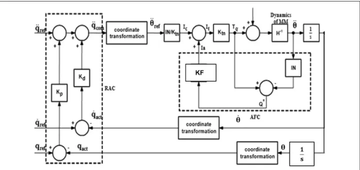
The path of the mobile robot is controlled using resolved-acceleration control (RAC), AFC and RAC-AFC-KF strategy. In RAC-AFC-KF, there are two feedback loops in the control scheme, the so-called external and internal loop as in Figure 2; the external loop is used for controlling the kinematic para-meters by the RAC, and the internal loop is used for controlling the dynamics of robot through the AFC controller. KF is used to eliminate the noises and uncertainties from the measurements.

RAC control strategy

This controller is working based on minimizing of the position and orientation errors to zero, which needs to apply suitable torque or forces to the system using the following equation

@2

@t2ðxrefxactÞ þK1

@

@tðxrefxactÞ þK2ðxrefxactÞ ¼0 ð13Þ

whereK1, K2are scalar constants related to the input torque

of the system. Xact and Xref are the actual and reference trajectories, respectively.

Figure 2.A schematic of the RAC-AFC-KF controller. RAC: resolved-acceleration control; AFC: active force control; KF: Kalman Filter.

AFC control strategy

AFC controller is the inner loop of the proposed controller, and it is mainly dependent on the angular acceleration feed-backs of the of wheel motors.

In the real-world environment, AFC controller can be described as the torque signal applied to actuators that drive the wheels based on the measured angular acceleration of the wheels via the sensors. The product of the measured acceleration with the estimated inertial matrix (IN) signal was compared with the applied torque (t) as in equation (14). By estimating the inertia matrix using suitable tech-nique, the controller can compensate effectively the effect of the disturbances. In simulation, the measurements are assumed to be ideal (perfect modelling). The equation that is used to estimate the disturbances can be written as in equation (14)

t_d¼tI N€q ð14Þ

wheret_dis the estimated torque disturbance effected on the wheels.tis the actuated torque that can be calculated in the case of a DC torque motor using the equation: t ¼Kt I whereKt is the torque constant of the DC motor,Iis the armature current and IN is the estimated inertia matrix, which has to be estimated well during the robot movement.

Estimation of inertial matrix

The estimation of the inertia matrix is necessary to compute the actual torque of the WMR from the disturbance torque obtained using equation (15) for the AFC control action. The moment of inertia must be appropriately estimated. As a rule of the thumb, the initial values of the elements inIN are assumed to be the values of M(q) computed by the dynamic model or lie within a suitable range18as in equa-tion (15)

0:4MðqÞ<IN<1:4MðqÞ ð15Þ

There are many methods that can be used to calculate the inertia matrix during the robot movement such as crude approximation14,16 and artificial intelligence (AI) approaches, e.g. NN,18 iterative learning,19 knowledge-based21and FL.22Since the inertia matrix typically has a known range as expressed in equation (16), it is sometimes preferred to use the FL controller. In addition,is the only variable inM(q) that is instrumental for the inertia matrix estimation. Thus,was chosen as the input set of the FL system whileINfor both the right and the left wheels of the WMR were assigned as the outputs. As a result, we have only three variables as the input and output of the FL which can be adjusted. More variables will lead to complex fuzzy system while less sets leads to inaccurate FL modelling. The FL system then calculates the estimatedINnecessary for the computation of the actual torque of the AFC con-troller for a given set of inputs. FL methodology passes through the following steps:

Fuzzification: In this process the crisp values is trans-formed into fuzzy values through finding the linguistic variables of the fuzzy set and determining the suitable membership function to arrange the relation between these variables. Thus, the mass matrix,M(q) in equation (12), can vary accordingly to the changes in sin () and cos(), we choseas the input to FL, which was fuzzi-fied into the following linguistic terms:

¼[Very Low, Low, Medium, High, Very High] Figure 3. shows the membership functions of the input and output sets.

The output of the FL is fuzzified into the following linguistic variables:

INR/INL¼ fVery Small, Small, Medium, Large, Very Largeg

It was found after some trials that the triangular shapes of the membership functions are suitable for calculating the value of the inertia matrix.

Rule Interface: It is used to define the relationship between the crisp input and output through the linguistic expressions (if–then statements) based on two approaches, namely,SugenoorMamdani. In this simu-lation, the fuzzy interface system is using theMamdani type as follows:

1. If(phi is M)then(INR is MR)&(INL is ML) 2. If (phi is VL) then (INR is VSR)&(INL is

VLL)

3. If(phi is L)then(INR is SR)&(INL is LL) 4. If(phi is H)then(INR is LR)&(INL is SL) 5. If (phi is VH) then (INR is VLR)&(INL is

VSL)

Defuzzification: All fuzzy outputs are aggregated using the centroid weighted method and the fuzzy output is trans-formed into a crisp output. In this simulation, the centroid method is used for defuzzification using equation (16)

x¼

ð

iðxÞxdx

iðxÞdx

ð16Þ

Stability analysis of RAC-AFC

According to the Lagrange equation, the torque of dynamic system is given by equation (12).

The dynamic system with the closed-loop feedback compensation as shown in Figure 2 can be calculated by equation (17)

MðqÞð€q_d þ kde_qþkpeqÞ þet ¼t ð17Þ

With equality of torque of robot as in equation (12) with the estimation torque using equation (17), one will get

By simplifying equation (18), one can get € eqþ kde_qþkpeq¼MðqÞ1 Vðq;q_Þ et ð19Þ

Lemma. Let V(t) is the Lyapunov function of the continuous-time control system. If V(t) is satisfying the differential inequality as in equation (20)

_

V aV þgðtÞ ð20Þ

whereais a positive constant.gðtÞis a function based on time which has positive values whent>0and can achieve the condition lim

t!1gðtÞ ¼C, this will guarantee that the closed loop will reach the global uniform ultimate bound-edness for any value oft.

Theorem.The mobile robot control based on equation (7) with noises is considered. Ifet_ is bounded, then the con-troller that was derived based on RAC and AFC, with equations (14) and (15), respectively, could guarantee to

reach the global uniform ultimate boundedness of the closed-loop scheme with exponential-convergence-rate.

Proof. Let’s have the following constants with positive values as follows: k1¼diag½k11;. . .:kn1>I5; k2¼ diag½k12;. . .:kn2>I5; k3¼diag½k13;. . .:kn3>I5; k3> k2, where I5is 5 5 identity matrix. kp¼diag½k1p;. . .: knp; kd ¼diag½k1d;. . .:knd

k5¼ jk1þkdMðqÞ1k2j, k6¼ jkpMðqÞ1k3j, k7¼ jk6k5k1j, k8¼ jk2kdk3j, k9¼ jMðqÞ1k2þ k8j, k10¼ jkpk2þMðqÞ1k2k8k1j, where k5–k10 are 55 matrices.

In RAC-AFC controllers as shown in Figure 2, we have three loops of errors; first loop withKphas an error equal to

eq. The errors in the second loop with Kd and third loop

with AFC can be calculated as equations (21) and (22), respectively x¼e_qþk1eq ð21Þ y¼etþk2e_qþk3eq ð22Þ 0 50 100 150 200 250 300 350 0 0.2 0.4 0.6 0.8 1 phi Degree of membership M L VL VS S

(a)

(b)

(c)

Figure 3.Fuzzy logic membership functions: (a) membership function of the fuzzy input set (); (b) membership function of the fuzzy output set (INL); (c) membership function of the fuzzy output set (INR).

The structure of KF-RAC-AFC feedback loops allows to eliminate robustly the effects of errors, in which the inner loops are compensating the errors very fast, with 10 times or higher than the outer loops.29Thus one can write

jeqj je_qj jetj

If we consider thatk1,k2andk3are larger than identity matrix, andk3is larger thank2as mentioned previously, the plus/minus sign of eqterm will play the most significant

role to determine the signs ofxandyerrors as in equations (21) and (22). As a result of that, the xandyerrors will accordingly get the same sign eitherþor – along the con-troller operation time.

By deriving errorx

_

x¼€eqþk1e_q ð23Þ By substituting the value of€eq from equation (19)

_

x¼MðqÞ1Vðq;q_Þ et

kde_qkpeqþk1e_q By substituting the value ofet from equation (22)

_

x¼MðqÞ1ðVðq;q_Þ ðyk2e_qk3eqÞ kde_qkpeqþk1e_q

By collecting the identical parts

_ x¼MðqÞ1Vðq;q_Þ yk1þkdMðqÞ1k2 _ eq kpMðqÞ1k3 eq _ x¼MðqÞ1Vðq;q_Þ yk5e_qk6eq

By substituting the value ofe_q from equation (21)

_ x¼MðqÞ1Vðq;q_Þ yk5ðxk1eqÞ k6eq _ x¼MðqÞ1Vðq;q_Þ yk5x ðk6k5k1Þeq _ x¼MðqÞ1Vðq;q_Þ yk5xk7eq By deriving errory _ y¼et_ þk2€eqþk3e_q ð24Þ By substituting the value of€eq from equation (19)

_ y¼e_tþk2 MðqÞ1Vðq;q_Þ et kde_qkpeq k3e_q ¼e_tþk2 MðqÞ1Vðq;q_Þ et kpeq ðk2kdk3Þe_q ¼e_tþk2 MðqÞ1Vðq;q_Þ et kpeq k8e_q

By substituting the value ofe_q from equation (21)

_ y¼e_tþk2 MðqÞ1Vðq;q_Þ et kpeq k8ðxk1eqÞ

By substituting the value ofet from equation (22)

_ y¼et_ þk2MðqÞ1ðVðq;q_Þ ðyk2e_qk3eqÞ k8xkpk2eqÞ k8k1eq ¼e_tþk2 MðqÞ1Vðq;q_Þ y MðqÞ1k2₂þk8x kpk2þMðqÞ1k2k3k8k1 eq ¼e_tþk2 MðqÞ1Vðq;q_Þ y k9xk10eq The quadratic Lyanupov function can be defined as follows V ¼1 2e 2 qþ 1 2x 2_þ1 2y 2_{þxy ð25Þ}

where x and y have the same þ/ sign as have been explained previously. Equation (25) can be written in the matrix form as follows

V ¼1 2e T qeqþ 1 2x T_xþ1 2y T_yþxT_y _ V ¼eqe_qþxx_þyy_þxy_ þxy_ ð26Þ Equation (26) can be written in the matrix form as follows _ V¼eT qe_qþxTx_þyTy_þyTx_þxTy_ ¼eT qðxk1eqÞ þxT MðqÞ1 Vðq;q_Þ yk5xk7eq þyT_{e_} tþk2 MðqÞ1 Vðq;q_Þ y k9xk10eq þyT_M ðqÞ1Vðq;q_Þ yk5xk7eq þxT_{e_} tþ k2 MðqÞ1 Vðq;q_Þ y k9xk10eq ¼eT qxe T qk1eqþxTMðqÞ1Vðq;q_Þ xTMðqÞ1y xT_k 5xxTk7eqþ yTe_tþyTk2MðqÞ 1 Vðq;q_Þ yT_k 2MðqÞ 1 y yT_k 9xyTk10eq þyTMðqÞ1Vðq;q_Þ yTMðqÞ1yyTk5xyTk7eq þxT_{e_} tþxTk2MðqÞ1Vðq;q_Þ xTk2MðqÞ1yxTk9xxTk10eq ¼ eT qk1eqxTðk5þk9Þx yTMðqÞ1ðk2þ1Þ xT_MðqÞ1 ðk2þ1ÞyyTðk9þk5Þxþ eT q xþx T_MðqÞ1 Vðq;q_Þ xT_k 7eqþyTet_þyTk2MðqÞ1Vðq;q_Þ yTk10eqþyTMðqÞ1Vðq;q_Þ yT_k 7eqþxTet_þxTk2MðqÞ1Vðq;q_Þ xTk10eqÞ

Ifet_ is changing with a constant rate and fixed sampling time in the whole experiment, this will boundet_ as follows

ket_ kd

wheredis the first derivative of the torque error.

IfM(q) orINis bounded in a FL system as in equation (15), and’_2inVðq;q_Þis also changed with a constant rate

ð’_ ¼constantÞ, this will cause the ratioMðqÞ1Vðq;q_Þis also bounded too.

The derivation ofLyapunovfunction as in equation (26) can then be written as

_

whereais the minimum factors ofx,yandxy. C¼Sup t!1 ðe_qTxþxTMðqÞ1Vðq;q_Þ xTk7eqþyTet_ þyTk2MðqÞ1Vðq;q_Þ yTk10 eqþyTMðqÞ1Vðq;q_Þ yT_k 7eqþxTe_tþ xTk2 MðqÞ1Vðq;q_Þ xTk10eqÞ According to the above-mentioned Lemma, the closed-loop control system is guaranteed to reach the global uniform ultimate boundedness with exponential-convergence-rate ofVspecified by a:

Path control simulation

The simulation is accomplished considering a roundabout setting in MATLAB [R2016a] computing environment, where the robot is navigating autonomously from starting to goal positions. The RAC-AFC control scheme has been applied to enable the robot to track the planned path with small tracking errors.

Mobile robot path planning

With the novel path planning algorithm, the so-called laser simulator graph search approach,28,30,31,32the collision-free path is determined in a roundabout environment. The start and goal points of the path are pre-chosen by the user to drive the robot in a roundabout with 360rotation while avoiding the obstacles as shown in Figure 4.

Robot path control

The simulation for the predefined path as shown in Figure 4(b) was performed using MATLAB/Simulink according to the following conditions:

Integration algorithm:BogackiShanpine Simulation type: Fixed step size

WMR parameters:r¼0.15 m,b¼0.75 m,d¼0.03 m,m

¼31.0 kg,mw¼0.5 kg,I¼15.625 kg m2,Iw¼0.005 kg m2 Controller parameters:Kpx¼2/s2,Kpy¼2/s2,Kp¼2/s, Kdx ¼1, Kdy ¼Kd ¼1 (for the RACpart), Kt ¼[0.265 0.265]T

N/A (obtained from datasheet for the DC motor) Several disturbances with constant and harmonic tor-ques were applied at both left and right wheels of the robot to test the performance of the control system. Three types of controllers were used in the simulation work, namely, the RAC-based kinematic controller, AFC-based dynamic controller and RAC-AFC controller, which were subse-quently compared using a referenced trajectory.

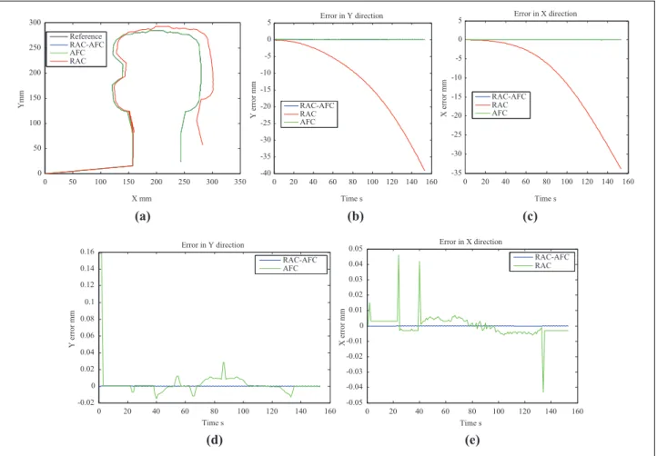
Figure 5 shows the actual trajectory of all the control-lers without disturbance during the robot tracking along the predefined path as depicted in Figure 4. RAC presents the reckoning errors that are incrementally increased dur-ing the trackdur-ing of the path with high trackdur-ing errors of about 30 mm and 35 mm inx and yaxes, respectively. However, the differences between the referenced and

actual paths generated by the AFC and RAC-AFC schemes are too small; the tracking errors were in the region of 102mm.

It was noticed that large initial errors (overshoots) occurred at the beginning of the simulation period for the AFC controller since there are as yet still no output signals received from the AFC controller loop at that point in time, whereas for the RAC and RAC-AFC schemes, there was no noticeable overshoots due to the positive effects of the kinematic control action at the beginning of the motion.

Figure 6 shows the actual trajectory of all the three controllers with the application of constant disturbance tor-ques to both wheels, td¼ ½0:1 0:1T Nm as the mobile robot navigates the predefined path.

For the second case of applying harmonic disturbance torques at both wheels with td ¼ [10000 sin(t) 10000 cos(t)]TNm, the RAC approach presents big deviation in the errors of about 50 mm and 60 mm inxandydirections, respectively, during tracking. Similar to the first case, the tracking errors for the AFC and RAC-AFC controllers remain very small, also in the region of 102mm for both xandydirections. Figure 7 shows the actual trajectory of the AFC and RAC-AFC controllers with harmonic distur-bance applied to the robot moving in the same the prede-fined path as shown in Figure 4.

The third case considers only the AFC-based schemes. The performance of such systems in terms of the track-ing errors is quite obvious; the errors for the AFC control-lers are in the region of 102mm in thexandydirections, more so for the RAC-AFC scheme that exhibits much smaller tracking errors (about 103mm or less in both x andydirections).

Figure 8 shows a comparison between the actual trajec-tory of RAC-AFC controller and reference trajectrajec-tory without and with harmonic disturbances,td ¼½10;000 cosðtÞ10;000sin tþp

2

TNm applied to both wheels of the mobile robot. The tracking errors with/without disturbance are too small. The tracking errors in the x direction for RAC-AFC with/without disturbance are illustrated in Fig-ure 8(a) are in the region of 104mm with maximum errors of 2.5104mm and 0.5104mm with and without disturbances, respectively. In theydirection, the tracking

Figure 4.Predefined path of mobile robot: (a) principle of laser simulator; (b) free-collision path with one obstacle.

errors have maximum value of about 5104mm and 4

104mm with and without disturbances, respectively, as shown in Figure 8(b). It can be said that the RAC-AFC controller shows a higher degree of disturbance rejection among all controllers.

Experimental path control

The mobile platform was set to move at a relatively low speed, typically in the range of 0.2–1.5 m/s. This range is in fact applicable to vehicles that are normally used for road

0 20 40 60 80 100 120 140 160 -0.02 0 0.02 0.04 0.06 0.08 0.1 0.12 0.14 0.16 Time s Y error mm Error in Y direction RAC-AFC AFC 0 20 40 60 80 100 120 140 160 -0.05 -0.04 -0.03 -0.02 -0.01 0 0.01 0.02 0.03 0.04 0.05 Time s X error mm Error in X direction RAC-AFC RAC (d) (e) 0 50 100 150 200 250 300 350 0 50 100 150 200 250 300 X mm Ymm Reference RAC-AFC AFC RAC 0 20 40 60 80 100 120 140 160 -40 -35 -30 -25 -20 -15 -10 -5 0 5 Time s Y error mm Error in Y direction RAC-AFC RAC AFC 0 20 40 60 80 100 120 140 160 -35 -30 -25 -20 -15 -10 -5 0 5 Time s X error mm Error in X direction RAC-AFC RAC AFC (a) (b) (c)

Figure 5.Results of the RAC, AFC and RAC-AFC controllers without disturbance: (a) trajectory of mobile robot; (b) y track errors for all controllers; (c) y track errors for AFC and RAC-AFC; (d) x track errors for all controllers; (e) x track errors for AFC and RAC-AFC. RAC: resolved¼acceleration control; AFC: active force control.

0 50 100 150 200 250 300 350 -50 0 50 100 150 200 250 300 x mm y mm Referenc RAC-AFC AFC RAC 0 20 40 60 80 100 120 140 160 -50 -40 -30 -20 -10 0 10 20 Time s Y error mm Error in Y direction RAC-AFC RAC AFC 0 20 40 60 80 100 120 140 160 -80 -60 -40 -20 0 20 40 Time s X error mm Error in X direction RAC-AFC RAC AFC (a) (b) (c)

Figure 6.Results of the RAC, AFC and RAC-AFC controllers with disturbance, 0.1 Nm at both wheels: (a) trajectory of mobile robot; (b) x track errors; (c) y track errors. RAC: resolved-acceleration control; AFC: active force control.

service applications such as road painting, side road grass cutting and cleaning. A COM server communication was utilized to transmit and receive the data online through pro-gramming using Visual C-sharp [Visual C# 2010 Express] as client and MATLAB computing platform as the server.

The KF algorithm was computed in MATLAB via the samem-filescript, where the signal and image processing sections were numerically processed. The Simulink pro-gram was then linked to themfile for calculating the AFC parameters. Figure 9 shows the link between MATLAB (as server) and C-sharp (as client) using the COM automation server with appropriate connections to the sensors and actuators.

The path of the mobile robot is controlled using the RAC-AFC strategy as presented in the second section. Considering similar conditions with that of the path control simulation, two feedback loops were used in the control scheme, that is, the external and internal loops. The former is used for controlling the kinematic parameters by the RAC, while the latter for controlling the robot dynamics by the AFC controller. RAC controller is known as the outer loop of the RAC-AFC control system and in the AFC controller, the torque applied at the driving wheels was estimated in real time during movement. The encoders were used to numerically estimate the angular acceleration (via second derivative of the angular position) of the

0 20 40 60 80 100 120 140 160 180 -3 -2 -1 0 1 2 3 4x 10 -4 time s X track error m

x track error with disturbance x track error without disturbance

0 20 40 60 80 100 120 140 160 180 -5 -4 -3 -2 -1 0 1 2 3 4 5x 10 -4 time s Y track error m

y track error with disturbance y track error without disturbance

(a)

(b)

Figure 8.Results produced by the RAC-AFC controller for both with and without disturbances: (a)x-tracking errors; (b)y-tracking errors. RAC: resolved-acceleration control; AFC: active force control.

-50 0 50 100 150 200 250 300 -50 0 50 100 150 200 250 300 X mm Ymm Reference RAC-AFC AFC 0 20 40 60 80 100 120 140 160 -0.02 0 0.02 0.04 0.06 0.08 0.1 0.12 0.14 0.16 Time s y error mm Error in Ydirection RAC-AFC AFC 0 20 40 60 80 100 120 140 160 -0.05 -0.04 -0.03 -0.02 -0.01 0 0.01 0.02 0.03 0.04 0.05 Time s X error mm Error in X direction RAC-AFC AFC (a) (b) (c)

Figure 7.Results of the AFC and RAC-AFC controllers with harmonic disturbancetd¼

10000sinðtÞ 10000cosðtÞ

Nm: (a) trajectory of mobile robot; (b)xtrack errors; (c)ytrack errors. RAC: resolved-acceleration control; AFC: active force control.

wheels. The signals were then multiplied with the esti-mated inertia matrix to calculate the required actuated torque, again through a signal processing task. This signal in turn is compared with the applied torque as expressed in equation (14). The torque of the selected DKM-DC motor used in this project has a linear relationship with the cur-rent and angular speed characteristic as shown in Figure 10. Note that the torque was calculated according to the angular speed characteristic. By getting the speed from encoders and taking into consideration the gear ratio, the equation that calculates the applied torque can be written as follows

t¼Knn ð28Þ

where Kn is a torque constant, the value of which is obtained as 0.00108 Nm/r/min after unit conversion and derived from the datasheet of the selected motor (see Figure 10). m ¼1:30 is the gearbox ratio, again taken from the catalogue of the selected motor.nr/min is the speed of the wheel measured by the encoder which can be calculated as follows

n¼ Pcur

T Prf ð29Þ

wherePcuris the number of pulses for the whole move-ment of robot from the start to current positions, Prf is the number of pulses for one full rotation, T is the period (or sampling time) from the start to current posi-tions. Thus, by getting the encoders measurements and then multiplied them with Knand m, the applied torque computed by the DC motors can be estimated and con-trolled. The acceleration can be calculated from the encoders’ measurements as second derivatives of the positions between two successive measurements as for-mulated in equation (30)

a¼@2ðx2x1Þ

@T2 ð30Þ By estimating the inertia matrix using a suitable method, the controller can effectively compensate the disturbances. In this practical experimentation, FL method was also

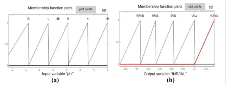
implemented. The disturbances in the AFC controller can be estimated using equation (14). The FL linguistic vari-ables and membership functions, which were used to esti-mate the inertia matrix are shown in Tables 1 and 2 and Figure 11.

The input fuzzy set is:

¼ fVery Low, Low, Medium, High, Very Highg

The output fuzzy sets are:

INR/INL ¼ fVery Small, Small, Medium, Large, Very Largeg

Propagation of kinematic uncertainty using KF

In the process state, the state variable vector,q¼[x, y,

]Tis calculated by the average velocity as expressed in equation (31). The direct KF was implemented in which the measurement signals from the odometry device, camera and LRF were combined and transformed into a single measurement vector, Zk as presented in equation (33), which is then fed into the KF algorithm. The linear discrete

LRF Camera MAT LAB Visual C# COM Automation server Motor Driver (Smart-Drive 40) Encoders IFC Cards φ Motors & wheels

Figure 9.Software communication with sensors and actuators.

time of the state variable that describes the time update step for the KF can be written as follows

q_k ¼Aq_k1þBukþBw ð31Þ

If the sampling period is small enough and both the linear and angular velocities are assumed to be constant throughout the duration, the position state variable of the non-holonomic WMR within its environments in the pres-ence of the uncertainties in discrete time is

xk y_k ’k 2 6 4 3 7 5¼ 1 0 0 0 1 0 0 0 1 2 6 4 3 7 5 xk1 y_k1 ’k1 2 6 4 3 7 5þ rT cosð’Þ dsinð’Þ sinð’Þ dcosð’Þ 0 1 2 6 4 3 7 5 Vþwv _ ’þw’: " # ð32Þ

The KF measurement equation with noise is

Zk¼C qkþvk ð33Þ

The equation that describes the sensor model in WMR is thus x_k y_k ’_k 2 6 4 3 7 5¼ 1 0 0 0 1 0 0 0 1 2 6 4 3 7 5 xkfrom LRF y_kfrom odometry

’_kfrom mixed LRF; Odometry and LS 2 6 4 3 7 5þ v1 v2 v3 2 6 4 3 7 5 ð34Þ

In the real-world application, the values ofQkandRk are not constant and always changing with each time step.

Thus, the actual process and measurement noises are not a zero-mean white noise which in turn renders the residual in KF a non-white noise. For this reason, the KF would diverge or tend to produce a large bound. To avoid this condition, the exponentially weighted moving averages were used to estimate the discrete time-varying system covariance from the noisy measurements in KF33 as follows

Rk ¼Rxk1andQk¼Qxk1 wherex>1 ð35Þ Note thatQandRare constant values. In this study, we assumeQ¼[0.001 0.001 0.001]TandR¼[1 1]Tafter a number of trial runs. For different values ofx(from 1 to 5), the mean trajectory errors after applying KF are computed as shown in Table 3.

From the table,xis chosen as 3 since KF produces the smallest divergence.

The KF gain that shows how much the estimation must be corrected can be computed from the measurement using

Kk¼PkC T_ðCP

kC T_þR

kÞ1 ð36Þ A posteriori state is generated by incorporating the mea-surement with the priori values of the state variable as

q_k ¼q_k þKkðZC qkÞ ð37Þ The priori and posteriori error covariance estimations can be calculated from equations (38) and (39), respec-tively, as follows

P_k ¼APk1ATþQk ð38Þ Pk¼ ðIKkCÞPk ð39Þ

Experimental results and discussion

The laser range finder, encoders and cameras data as in previous studies24–26were used to localize, determine the path and control the robot in a road roundabout environ-ment as shown in Figure 12.

The image processing algorithm consists of two main parts; that is, preprocessing of the image and processing of the image and local map building. The image processing algorithm is listed here and more details can be found in previous studies,28,34

(i) Preprocessing of the image

The main operations that were used in this phase are listed as follows:

– Constructing the video input object – Preview of the Wi-Fi video

Table 1.Fuzzy input variable,

Variable:() Very low (VL) 6.7 to4.8 Low (L) 4.8 to3.3 Medium (M) 3.3 to1.9 High(H) 1.9 to0.45 Very high (VH) 0.45 to 1

Table 2.Fuzzy output variables, INL and INR. Variables: INL and INR [kg m2_]

Very small (VS) 0.27–0.30

Small (S) 0.30–0.33

Medium (M) 0.33–0.36

Large (L) 0.36–0.40

– Setting the brightness of live video – Start acquiring frames

– Acquiring the image frames to MATLAB

workspace – Crop image

– Convert from RGB to grayscale

– Remove image acquisition object from memory (ii) Processing of the image and development of the

environments local map

It includes some operations that allow the extraction of the road edges and roundabout from the images with capa-bility to remove the noises and perform filtration. The fol-lowing operations were applied for edge detection and noise filtering:

– 2-DGaussianfilters

– Multidimensional images (imfilter) – Prewittfilter for edge detection – Morphological operations:

Morphological structuring element: It is used to define the areas that will be applied using morphological opera-tions. Straight lines with 0and 90are the shapes used for the images which actually represent the road curbs.

Dilation of image: In the dilation process, a number of pixels are added to the boundaries of the objects in the image, which depends on the size and shape of the structur-ing element that is used to process the image.

BWCis the binary image coming from the edge filters. – 2-D order-statistic filtering

– Removing of small objects from binary image – Filling of the image regions and holes

The results of the preimage and image processing are illustrated in Figures 13 and 14.

The signal measurements of the odometry and LRF were used to estimate the position and orientation of the robot in road following and roundabout environments with 360 rotation as shown in Figure 15. These mea-surements include some unexpected noises and errors

Table 3.Empirical calculation ofx.

x

Mean difference between the trajectory before and after using KF (mm)

1 31.3 2 28.8 3 26.7 4 29.6 5 30.5 KF: Kalman Filter.

Figure 12.Outdoor roundabout environment: (a) Road round-about and (b) mobile robot platform used in the experiments.

Figure 11.FL rule interface and membership functions of the FL system with reference to the input and output: (a) input (); (b) output INR/INL. FL: fuzzy logic.

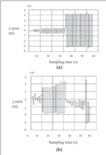
that can be effectively avoided after using KF and RAC-AFC controller. Figures 15(b) to (d) show the effect of applying KF with AFC controller to enhance the robot path in comparison with the path planning from signal measurement. Figure 16 shows the track errors of RAC-AFC controller in which for thexdirection, a maximum error of about 7 105 mm is attained as shown in Figure 16(a).

However, in y direction, the maximum track error is around 6104mm (Figure 16(b)). Although the experi-ments show that the complete navigation method enables the robot to move smoothly in the road environments in comparison to the direct path execution, the resulted path is not smooth and contains many ripples that may be due to the time needed to perform the path planning, localization and control calculations

The parameters used in the calculation are as follows: WMR parameters:r¼105.4 mm,b¼500 mm,d¼16.5 mm, m¼ 36 kg,mw¼ 1.5 kg, I ¼10.0567 kg m2, Iw ¼ 0.0083 kgm2,V¼0.15 m/s; Controller parameters:Kpx¼2/s2,Kpy¼2/s2,Kp¼2/s, Kdx¼Kdy¼Kd¼1,Kn¼0.00108 Nm/r/min.

Conclusion

The RAC, AFC, RAC-AFC and RAC-AFC-KF controllers were used to navigate the robot and track the predefined roundabout trajectory both in simulation and in experimen-tal studies. The parameters of the controllers were derived from the kinematic and dynamic models that fully describe the mobile robot motion with non-holonomic constraints. The FL reasoning was implemented to estimate the inertia matrix leading to the computation of the applied torque to

Figure 13.Navigating on the road following section in indoor environment using camera image sequences: (a) original image in the first iteration, (b) image after preprocessing and processing at the start position, (c) image after preprocessing and processing at the goal position path.

Figure 14.Camera sequence images when navigating in outdoor environment with 360rotation (a) image when start moving, (b) camera’s local map when robot starts to move, (c) camera’s local map when robot detects the roundabout.

Figure 15.Path of mobile robot during navigation through the roundabout environment: (a) comparison between the path acquired from sensors signals before and after using KF and AFC controller, (b) comparison between the KF path and RAC-AFC controller, (c) KF path, (d) RAC-AFC controller path. RAC: resolved-acceleration control; AFC: active force control; KF: Kalman Filter.

drive the WMR wheels. From the results of simulation, it looks as if there are no noticeable errors for without dis-turbance condition. However, a small deviation (error) was observed with the application of constant or harmonic dis-turbances. In the experimental works, a drift between the actual and reference paths occurred due to the delay in processing the data from the sensors and noises, the latter of which were eliminated using KF. In conclusion, it is shown that the RAC-AFC-KF controller has demonstrated its capability to eliminate the disturbances and noises from the system both in simulation and experimental works.

Declaration of conflicting interests

The author(s) declared no potential conflicts of interest with respect to the research, authorship, and/or publication of this article.

Funding

The author(s) received no financial support for the research, authorship, and/or publication of this article.

ORCID iD

Mohammed AH Ali https://orcid.org/0000-0002-5179-7027

References

1. Asif M, Khan M, Safwan M, et al. Feedforward and feedback kinematics controller for wheeled mobile robot trajectory tracking.J Autom Control Eng2015; 3(3): 178–182. 2. Gunes M and Baba F. Speed and position control of

autono-mous mobile robot on variable trajectory depending on its curvature.J Sci Ind Res2009; 68: 513–521.

3. Lee TH, Hung FHF and Tam PKS. Position control for

wheeled mobile robots using a fuzzy logic controller. Hong Kong: The Hong Kong Polytechnic, University, Hung Hom, Kowloon, 2002.

4. Astudillo L, Castillo O, Melin P, et al.Intelligent control of an autonomous mobile robot using type-2 fuzzy logic. Mex-ico: Division of Graduate Studies and Research in Tijuana Institute of Technology, 2006.

5. Velagic J, Osmic N and Lacevic B. Neural network controller for mobile robot motion control.World Acad Sci Eng Technol 2008; 2(11): 47.

6. Borensteinand J and Koren Y. Motion control analysis of a mobile robot.J Dyn Sys Meas Control1987; 109(2): 73–79. 7. Mester G. Intelligent mobile robot motion control in unstruc-tured environments. Acta Polytechnica Hungarica 2010; 7(4): 153–165.

8. Kanayama Y, Kimura Y, Miyazaki F, et al. A stable tracking control method for a non-holonomic mobile robot. In: Pro-ceeding IEEE/RSJ international workshop on intelligent robots and systems, Osaka, Japan, 3–5 November 1991, pp 1236–1241. IEEE.

9. Blochs A.Drakunov stabilization of a non-holonomic system via sliding modes. In:Proceedings of the 33rd Conference on Decision and Control, Lake Buena Vista, FL, 14–16 Decem-ber 1994. IEEE.

10. Chwa D. Sliding-mode tracking control of non-holonomic wheeled mobile robots in polar coordinates. IEEE Trans Contr Syst Trans2004; 12(4): 637–644.

11. Fierro R and Lewis FL. Control of a non-holonomic mobile robot: back stepping kinematics into dynamics.J Robot Syst 1997; 14(3): 149163.

12. Fukao T, Nakagawa H and Adachi N. Adaptive tracking con-trol of a non-holonomic mobile robot. IEEE Trans Robot Autom2000; 16(5): 609–615.

13. Jiangt Z and henk N. Tracking control of mobile robots: a case study in back stepping. Automatica 1997; 33(7): 1393–1399.

14. Hendzel Z. An adaptive critic neural network for motion control of a wheeled mobile robot. Nonlinear Dyn 2007; 50: 849.

15. Fateh MM and Arab A. Robust control of a wheeled mobile robot by voltage control strategy.Nonlinear Dyn2015; 79: 335. 16. Hewit JR and Burdess JS. Fast dynamic decoupled control for robotics using active force control.Trans Mech Mach Theory 1981; 16(5): 535–542.

17. Hewit JR and Marouf KB. Practical control enhancement via mechatronics design.IEEE Trans Ind Electron1996; 43(1): 16–22.

(a)

(b)

Figure 16.Track errors of the RAC-AFC controller: (a)x-track errors (b)y-track errors. RAC: resolved-acceleration control; AFC: active force control.

18. Mailah M.Intelligent active force control of a rigid robot arm using neural network and iterative learning algorithms. PhD Thesis, University of Dundee, UK, 1998.

19. Kwek LC, Wong EK, Loo CK, et al. Application of active force control and iterative learning in a 5-link biped robot. J Intell Robot Syst2003; 37: 143–162.

20. Luh JYS, Walker MW and Paul RPC. Resolved acceleration control of mechanical manipulator. IEEE Trans Automat Contr1980; 25: 486–474.

21. Pitowarno E, Mailah M and Jamaluddin H. Knowledge-based trajectory error pattern method applied to an active force control scheme.IIUM Engineering Journal2002; 3(1): 1–15. 22. Tang HH, Mailah M and Jalil MKA, Robust intelligent active force control of non-holonomic wheeled mobile robot. J Teknologi2006; 44(D): 4964.

23. Luy NT. Omnidirectional vision-based distributed optimal tracking control for mobile multi-robot systems with kine-matic and dynamic disturbance rejection. IEEE Trans Ind Electron2018; 65(7): 5693–5703.

24. Luy NT. Robust adaptive dynamic programming based online tracking control algorithm for real wheeled mobile robot with omni-directional vision system.Trans Ins Meas Control2017; 39(6): 832–847.

25. Luy NT. Reinforcement learning-based intelligent tracking control for wheeled mobile robot.Trans Ins Meas Control 2014; 36(7): 868–877.

26. Chao C, Chengrui Z, Tianliang H, et al. Model-assisted extended state observer-based computed torque control for

trajectory tracking of uncertain robotic manipulator systems. Int J Adv Robot Syst2018; 15(5): 1–12.

27. Boukattaya M, Mezghani N and Damak T. Computed-torque control of a wheeled mobile manipulator.Int J Robot Eng 2018; 3(5): 1–6.

28. Mohammed AHA. Autonomous mobile robot navigation and control in the road following and roundabout environments incorporating laser range finder and vision system. PhD The-sis, Universiti Teknologi Malaysia, Malaysia, 2014. 29. William SL.Control system applications. Boca Raton: CRC

Press, Technology & Engineering, 2018.

30. Mohammed AHA, Mailah M and Hing TH. Path navigation of mobile robot in a road roundabout setting. In:1st Interna-tional Conference on Systems, Control, Power, Robotics (SCOPORO’12) WSEAS, Singapore City, Singapore, 11–13 May 2012, pp. 198–203.

31. Mohammed AHA, Mailah M and Hing HT. Path planning of mobile robot for autonomous navigation of road roundabout intersection.Int J Mech2012; 6(4): 203–211.

32. Ali MAH and Mailah M. Laser simulator: a novel search graph-based Path planning.Int J Adv Robot Syst 2018; 15(5): 1–16.

33. Lewis F.Optimal Estimation with an introduction to stochas-tic control theory. New York: John-Wiley and Sons, 1986. 34. Ali MAH, Mailah M, Yussof WAB, et al. Sensors fusion

based online mapping and features extraction of mobile robot in the road following and roundabout.IOP Conf Ser Mater Sci Eng2016; 114(1): 012135.