Portland State University
PDXScholar
Geography Faculty Publications and Presentations
Geography
4-15-2017
Characterizing Large-Scale Meteorological Patterns and Associated
Temperature and Precipitation Extremes over the Northwestern
United States Using Self-Organizing Maps
Paul C. Loikith
Portland State University, [email protected]
Benjamin R. Lintner
Rutgers University
Alex Sweeney
Portland State University
Let us know how access to this document benefits you.
Follow this and additional works at:
https://pdxscholar.library.pdx.edu/geog_fac
Part of the
Geographic Information Sciences Commons
, and the
Physical and Environmental
Geography Commons
This Article is brought to you for free and open access. It has been accepted for inclusion in Geography Faculty Publications and Presentations by an authorized administrator of PDXScholar. For more information, please [email protected].
Citation Details
Loikith, P. C., B. R. Lintner, and A. N. Sweeney, 2017: Characterizing Large-Scale Meteorological Patterns and Associated
Characterizing Large-Scale Meteorological Patterns and Associated
Temperature and Precipitation Extremes over the Northwestern United States
Using Self-Organizing Maps
PAULC. LOIKITHDepartment of Geography, Portland State University, Portland, Oregon
BENJAMINR. LINTNER
Department of Environmental Sciences, Rutgers, The State University of New Jersey, New Brunswick, New Jersey
ALEXSWEENEYa
Department of Geography, Portland State University, Portland, Oregon
(Manuscript received 8 September 2016, in final form 20 December 2016) ABSTRACT
The self-organizing maps (SOMs) approach is demonstrated as a way to identify a range of archetypal large-scale meteorological patterns (LSMPs) over the northwestern United States and connect these patterns with local-scale temperature and precipitation extremes. SOMs are used to construct a set of 12 characteristic LSMPs (nodes) based on daily reanalysis circulation fields spanning the range of observed synoptic-scale variability for the summer and winter seasons for the period 1979–2013. Composites of surface variables are constructed for subsets of days assigned to each node to explore relationships between temperature, pre-cipitation, and the node patterns. The SOMs approach also captures interannual variability in daily weather regime frequency related to El Niño–Southern Oscillation. Temperature and precipitation extremes in high-resolution gridded observations and in situ station data show robust relationships with particular nodes in many cases, supporting the approach as a way to identify LSMPs associated with local extremes. Assigning days from the extreme warm summer of 2015 and wet winter of 2016 to nodes illustrates how SOMs may be used to assess future changes in extremes. These results point to the applicability of SOMs to climate model evaluation and assessment of future projections of local-scale extremes without requiring simulations to re-liably resolve extremes at high spatial scales.
1. Introduction
State-of-the-art climate models generally reproduce observed features of the mean large-scale climate and atmospheric circulation with reasonable fidelity, lending confidence to the ability of models to project changes in these features (Flato et al. 2013). Changes in mean cli-mate at large scales under anthropogenic greenhouse warming are typically projected with strong consensus across current-generation climate models (IPCC 2013). However, for many global and some regional climate models, skill is more limited at capturing phenomena
occurring at higher temporal or spatial scales, such as localized extremes, that may be influenced by small-scale geographical, topographical, or meteorological features not readily resolved at typical model resolu-tions (Seneviratne et al. 2012;Arritt and Rummukainen 2011;Walton et al. 2015). Projecting future climate at local scales with precision and confidence is therefore challenging, with limitations imposed by the computa-tional feasibility of long-term transient climate change simulations at sufficiently high resolutions to resolve local extremes. This challenge becomes greater in re-gions of complex topography and spatially heteroge-neous climate zones such as the northwestern United States (NWUS).
Weather and climate extremes are often associated with large-scale meteorological patterns (LSMPs) that drive processes (e.g., horizontal and vertical advection)
aCurrent affiliation: School of the Environment, Portland State University, Portland, Oregon.
Corresponding author e-mail: Paul C. Loikith, [email protected]
DOI: 10.1175/JCLI-D-16-0670.1
Ó2017 American Meteorological Society. For information regarding reuse of this content and general copyright information, consult theAMS Copyright Policy(www.ametsoc.org/PUBSReuseLicenses).
promoting the occurrence of extremes (Grotjahn et al. 2016, and references therein). LSMPs are synoptic-scale patterns defined in terms of key meteorological variables, including those related to circulation such as sea level pressure (SLP), or surface quantities like temperature. Because climate models are capable of resolving these features in many cases, LSMPs can be employed to evaluate model fidelity in producing synoptic conditions conducive to extremes, assess whether models capture extremes for plausible physical reasons, and interpret future changes in such conditions.
Composite analysis is one common way to define LSMPs associated with extremes and to interpret the physical mechanisms of extreme events at various scales in observations and climate models. For example,Dole et al. (2011) constructed composite LSMPs associated with the 2010 Russian heat wave, andMeehl and Tebaldi (2004) used composites in 500-hPa geopotential height (Z500) to identify the meteorology associated with the 1995 U.S. and 2003 European heat waves in observations and models.Grotjahn and Lee (2016)identified two types of LSMPs associated with heat waves over the Central Valley of California and found that model skill at re-producing these two patterns varied considerably across a suite of 14 global climate models (GCMs). LSMPs have also been linked to extreme precipitation events and used as a basis for model evaluation (e.g., DeAngelis et al. 2013;Gutowski et al. 2010;Kawazoe and Gutowski 2013). LSMPs as defined from composites are useful for characterizing extremes over relatively small or homo-geneous regions. However, LSMPs associated with ex-tremes at one location can differ considerably from those for other locations, even nearby ones, especially along coastlines or in regions of complex terrain. The assessment of composite patterns over large domains underscores the value of approaches that can extract common features from gridpoint-derived information.
Loikith and Broccoli (2012)implemented one such ap-proach by constructing ‘‘composites of composites’’ by centering reanalysis-derived extreme composites around a common origin. GCMs were also evaluated using this methodology and showed reasonable fidelity, especially in regions lacking complex topography (Loikith and Broccoli 2015). In a suite of regional cli-mate models,Loikith et al. (2015)found that models are still challenged over areas of complex terrain despite the relatively high 50-km spatial resolution. Employing empirical orthogonal function (EOF) analysis as a way to identify regions to construct LSMPs associated with extreme heat, Lau and Nath (2012, 2014) identified strong associations between extreme heat and anticy-clonic circulation anomalies over North America and Europe, respectively.
An alternative means to defining LSMPs (including those associated with extremes) is through application of self-organizing maps (SOMs; Sheridan and Lee 2011). SOMs comprise a class of unsupervised neural networks that organize input geospatial data (e.g., LSMPs) into a user-defined number of outputs (nodes) obtained by iter-atively adjusting the nodes to resemble the input data. SOMs are capable of distilling a large amount of data for LSMPs into an interpretable (small) set of nodes; in our usage, each node may be viewed as a characteristic LSMP. SOMs have been previously demonstrated as a useful tool in synoptic meteorology and climatology for characteriz-ing LSMPs and their associated impacts (e.g., Hewitson and Crane 2002) with specific applications including de-fining the continuum of SLP patterns over the entire Northern Hemisphere (Johnson et al. 2008;Johnson and Feldstein 2010), evaluating LSMPs in climate models (Cassano et al. 2006;Loikith and Broccoli 2015), identi-fying observed trends in dynamics linked to temperature extremes (Horton et al. 2015), and assessing future climate change behavior in model simulations (Radic´ et al. 2015). In the case of daily data analyzed here, each day is assigned to the node that is most similar (in a Euclidean distance sense) to the LSMP for that day. This allows for the association of characteristic LSMPs with other climate variables or impacts (e.g., extremes in temperature). In this way, SOMs have been used to interpret LSMPs associated with precipitation over South Africa (Lennard and Hegerl 2015) and temperature extremes over Alaska (Cassano et al. 2015,2016).
In addition to SOMs and composite analysis, LSMPs can also be characterized using synoptic typing ap-proaches, with clustering and EOF analysis as common methodologies. For example, over the western United States,Robertson and Ghil (1999)applied a probability density function bump-hunting method and k-means clustering to define a set of six synoptic regimes in 700-hPa geopotential height and linked the regimes with temper-ature and precipitation anomalies. Casola and Wallace (2007)clustered 500-hPa geopotential height patterns into four distinct regimes over the Pacific–North American sector. Sobie and Weaver (2012) used synoptic typing linked to precipitation patterns over Vancouver Island to statistically downscale climate projections of precipitation at local scales. The SOMs approach offers some advan-tages over clustering in that it treats the data as a con-tinuum, spanning the entire data space. The SOMs approach also identifies an array of direct synoptic states of the atmosphere and allows for detection of pattern mixing, whereas EOF analysis yields orthogonal modes based on variance (Reusch et al. 2005; Lennard and Hegerl 2015). In contrast to LSMPs constructed from
composites, LSMPs computed from SOMs are in-dependent of an index, which as noted is often defined at a particular location. Consequently, SOMs-derived LSMPs associated with extremes can be identified across an entire region with one set of maps. Furthermore, it is possible that distinct synoptic setups could lead to similar out-comes in terms of extreme events, which a simple com-posite analysis may not capture.
In this paper, we employ SOMs to describe the range of synoptic-scale circulation patterns over the NWUS in the current climate and connect these patterns to tempera-ture and precipitation extremes at local and/or regional scales. This work is further intended as a starting point toward using SOM-defined LSMPs, which are at scales easily achievable by current modeling capabilities, as proxies for extremes over the NWUS (in a probabi-listic sense) for climate model analysis and evalua-tion. The remainder of the paper is organized as follows. Section 2presents the data used. Section 3
describes the methodology including information on the SOM approach. Results are presented insection 4
followed by a discussion insection 5and conclusions insection 6.
2. Data
SLP, Z500, and 250-hPa wind speed (V250) are from the Modern-Era Retrospective Analysis for Research and Applications (MERRA) reanalysis (Rienecker et al. 2011). MERRA is a global reanalysis produced by the U.S. National Aeronautics and Space Administra-tion, provided at a1/28 32/38resolution every hour dating
back to 1979. Near-surface daily maximum and minimum temperature (Tmax and Tmin), downward shortwave ra-diation at the surface (DSRS), precipitation, and near-surface wind speed and direction are provided by the University of Idaho Gridmet dataset (Abatzoglou 2013). Gridmet gridded daily surface meteorological data are a hybrid observational dataset covering the contiguous United States from 1979 to the present on a 4-km grid. In situ station data are from the Global Historical Climatol-ogy Network–Daily product (GHCND;Menne et al. 2012). GHCND provides daily Tmax and Tmin, daily accumu-lated precipitation, and other meteorological variables. Anomalies were computed for Tmax and Tmin by re-moving the daily mean climatology from the entire period from each day. Anomalies for DSRS and precipitation were
FIG. 1. (left) Elevation and (middle) mean daily maximum temperature and (right) mean daily precipitation for (top) DJF and (bottom) JJA for the NWUS region. Note the changes in color scale between DJF and JJA. (Blue dots on the elevation map are locations of local-scale examples inFigs. 10and15.)
computed as percentages of the daily mean climatology. Analysis is performed over the 35-yr period 1979–2013.
3. Methodology
SOMs
SOMs have been demonstrated as useful and robust analytical tools for studying synoptic-scale meteorology in observations and climate models (Sheridan and Lee 2011; Hewitson and Crane 2002; Liu and Weisberg 2011). Several of the referenced studies include detailed descriptions of SOMs along with practical consider-ations for performing SOM analysis, so we only provide a brief overview here as it relates to this analysis. Many choices must be made in preparing the SOM, perhaps the most fundamental of which is the number of nodes. The choice of node number is often motivated by balancing the interest in representing a reasonably complete range of major patterns in the dataset (i.e., too few nodes will yield patterns that are too general) against considerations for interpreting the results (i.e., too many nodes can be cumbersome or impractical).
Previous studies have used a range of node numbers and arrangements. For example,Lennard and Hegerl (2015)
use a 334 node SOM (12 nodes) with multiple mete-orological fields as inputs.Cassano et al. (2015)argued that a larger SOM over a smaller domain provides op-timal interpretability over Alaska and Canada, and
Cassano et al. (2016)employed a relatively large 735 node SOM over Alaska. In this study, we use a rectan-gular 433 node SOM. We qualitatively assessed results obtained using both smaller and larger SOM arrays and found that a 433 configuration captured the range of synoptic-scale variability with sufficient detail to dis-tinguish among different variants of the same regime while being manageable for physical interpretation. The 12 nodes used here also contain preferred patterns for the occurrence of extremes at multiple point locations and across the domain. We use an initial neighborhood radius of 3 and a final neighborhood radius of 1 with 100 initial iterations and 300 final iterations.
We provide a multivariate SOM input, similar to the approach of Lennard and Hegerl (2015). SOM input comprises daily fields of SLP, Z500, and V250 to capture
FIG. 2. Climatological mean of (left) Z500, (middle) SLP, and (right) V250 for (top) DJF and (bottom) JJA. The domain plotted is the same as the input for the SOM.
near-surface, midtropospheric, and upper-tropospheric circulation, respectively. The multivariate SOM input provides a more complete set of dynamical information to the algorithm than a univariate input, and allows systematic interpretation of the LSMPs across different levels. The input domain is bounded on the north and south by 608 and 358N, respectively, and on the east and west by 1118and 1428W, respectively. The NWUS has strong seasonality in climate, so the SOM was performed separately on winter months, defined as December, January, and February (DJF; 90 days season21, excluding 29 February in leap years), and summer months, defined as June, July, and August (JJA; 92 days season21). At each grid point all input values of SLP, Z500, and V250 were first normalized by the temporal standard deviation to reduce the potential dispropor-tionate influence of one quantity. Next, all input data were weighted by the square root of the cosine of lati-tude to account for area differences across the grid points. The normalized and area-weighted SLP, Z500, and V250 data are then provided together as the input data to the SOM such that the SOM is trained over the three quantities simultaneously. In other words, the node assignment for any given day is valid for and de-termined collectively using all three input quantities. We found that the SOMs obtained for total fields yielded more readily interpretable results than those for de-seasonalized anomalies.
A Monte Carlo approach is used to determine whether the percentage of extreme events concurrent with each SOM node is statistically significant. The procedure is performed as follows: entire seasons of temperature and node assignments are sampled at random separately to construct a shuffled pair of time series. Then, the per-centage of extreme days concurrent with each node is computed. This process is repeated 1000 times on each grid point. Observed percentages that are greater than the 95th percentile of the synthetic probability distribution are considered statistically significant.
4. Results
The NWUS is characterized by complex topography, spatial climate heterogeneity, and a distinct seasonal cycle.Figure 1shows surface elevation and climatolog-ical means in temperature and precipitation from Gridmet. The moderating influences of the Pacific Ocean keep the coastal regions relatively mild during winter and summer (Fig. 1, middle). On average, inland areas are the coldest regions in winter and the warmest temperatures in summer are to the south, in the Co-lumbia River basin, and in the Snake River valley. The higher terrain of the Rocky Mountains and Cascades is
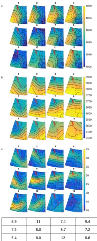
FIG. 3. DJF SOM patterns of (a) SLP (hPa), (b) Z500 (m), and (c) V250 (m s21) for each of the 12 nodes indicated above each panel. (bottom) The percentage of days assigned to each node out of a total of 3150 days is shown in the table.
cooler and wetter than surrounding valleys in both sea-sons. Winter experiences much greater precipitation than summer throughout most of the domain with the highest DJF precipitation amounts falling along the coastal mountains and Cascades, which create a rain shadow to their east.
Figure 2shows the climatological means in the SOM input fields (Z500, SLP, and V250) over the SOM input region. Winter climatology is characterized by an off-shore surface low, a strong 250-hPa jet weakening from west to east, and a subtle ridge axis along the coast at 500 hPa. In JJA, high pressure dominates offshore, with a Z500 trough axis along and just west of the coast, and a relatively weak 250-hPa jet overhead.
a. DJF
1) SOMRESULTS AND MEAN CLIMATE ASSOCIATIONS
Figure 3shows the SOM node patterns for DJF. The 12 maps for each variable show the composite mean for days assigned to the node, numbered as shown above
each panel and referred to as node 1 (N1), node 2 (N2), etc. The percentage of days (out of 3150) assigned to each node is shown at the bottom, with each cell in the chart corresponding to a node. N1 shows a surface low pressure centered to the northwest of the NWUS with a Z500 trough axis offshore and the main axis of the 250-hPa jet zonally oriented over central California. N12 (bottom right of SOM) is nearly opposite with a surface high pressure, an offshore Z500 ridge, and a 250-hPa jet arching to the north and east of the region. Patterns generally transition from N1 to N12 moving diagonally across the SOM. N10, which shares commonalities with the climatological mean in Fig. 2, and N7 have the highest frequency of pattern assignments with 11% and 10% of days, respectively, while N1 and N2 have the fewest with 6.7% and 6.8% days, respectively.
Figures 4,5, and6show composites of Tmin anomalies, precipitation anomalies, and the most frequent 10-m wind direction quadrant for days assigned to each node. For DJF, only Tmin is presented, as extreme cold daily low temperatures are arguably associated with the ma-jority of winter temperature impacts; Tmax composites
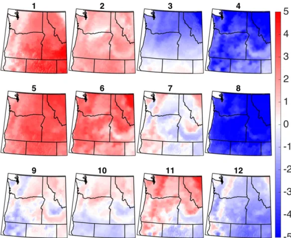
FIG. 4. Composites of DJF daily minimum temperature anomalies (K) for days assigned to each SOM node. Node numbers are indicated above each panel and correspond to the node numbering convention inFig. 3.
were also computed and shared many commonalities with Tmin. Wind direction is presented because of the important influence near-surface advection has on tem-perature; wind speed composites were also constructed but were less informative. Additionally, composites of surface insolation were constructed; however, the rela-tively short winter days and low sun angle diminish the role of insolation in the occurrence of temperature ex-tremes compared with the warm season (although nighttime cooling via longwave emission may be impor-tant in some cases).
Nodes in the upper left of the SOM (N1, N2, N5, and N6) tend to have positive Tmin anomalies throughout the NWUS. N1 and N5 also exhibit the highest domain wide positive precipitation anomalies. Patterns for N1 and N5 show an SLP gradient favorable for warm south or southwesterly flow near the surface, which is sup-ported by the predominant southerly wind component evident in Fig. 6. Combined with the offshore Z500 trough and strong 250-hPa jet, these nodes resemble those conducive to landfalling atmospheric rivers (ARs)
(Dacre et al. 2015;Ryoo et al. 2015). N2, while generally associated with warm conditions, exhibits negative pre-cipitation anomalies across most of the domain except along the southern tier. N6 is drier than average across the south and east and wetter than average over the northwest. The positive and negative precipitation anomalies align closely with the position of the 250-hPa jet as well as the centers of the Z500 ridge–trough pat-tern. Nodes on the right side of the SOM (N3, N4, N8, and N12) tend to be associated with negative tempera-ture anomalies, with N8 standing out as having the most widespread and largest amplitude anomalies. The LSMPs for these nodes vary, although all four have relatively high SLP. N8 exhibits a strong surface high to the north, promoting easterly winds, as suggested by
Fig. 6, and advection of cold inland air masses toward the coast. N8 and N12 also tend to be associated with very little precipitation across the NWUS (Fig. 5), while N3 and N4 have dry north–wet south anomaly patterns consistent with the southern location of the 250-hPa jet.
FIG. 5. Composites of daily DJF precipitation anomalies for each node. Anomalies are computed as a fraction of the climatological mean so a value of 1 indicates no deviation of the climatological mean. Node numbers are indicated above each panel and correspond to the node numbering convention used inFig. 3.
N7 shows generally cool anomalies in lower elevations and basins corresponding to conditions favorable for strong radiational cooling under a surface high and upper-level ridge. The opposite is true for N9 and N10 where valleys and basins tend be warmer than average while mountains are colder, suggestive of anomalously negative lapse rates. N9 has positive precipitation anomalies, while N10 shows positive precipitation anomalies in the northwest and northeast portions of the domain and a band of negative anomalies aligning with the Cascades rain shadow, a pattern indicative of oro-graphic precipitation. N11 is anomalously warm except for the southeast where ideal conditions for radiational cooling under the Z500 ridge and surface high may contribute to below-average minimum temperatures. This is consistent with the negative precipitation anomalies, which suggest the presence of dry air and clear skies. It is interesting to note for nodes that show a SLP gradient oriented from east to west (N1, N2, N3, N6, and N7), a common occurrence in winter in the re-gion, the corresponding panels inFig. 6depict the re-sulting relatively small-scale easterly winds through and
west of the Columbia River Gorge (indicated on maps with black circle), highlighting the benefit to connecting the synoptic-scale LSMPs with high-resolution obser-vations like Gridmet.
2) NODE FREQUENCIES BY YEAR
The yearly frequency of occurrence for each node is shown inFig. 7. El Niño–Southern Oscillation (ENSO) plays an important role in interannual climate variability across the region (Ropelewski and Halpert 1986). To see if the SOMs approach captures climate variability re-lated to ENSO, warm phase years are shown in red and cold phase years in blue, defined as years when the oceanic Niño index was greater than 1.0 or less than21.0, respectively. The bar second from the right, labeled ‘‘Clim’’ is the frequency of node occurrence for the entire 35-yr period.
There is a tendency for warm ENSO years to have higher frequencies of N1, N2, and to some extent N5 and lower frequencies of N4, N8, N9, N11, and N12. In
Fig. 3, N1 and N2 are associated with an amplified jet to the south, while N5 shows a strong jet axis oriented
FIG. 6. The mode of wind direction for days assigned to each node. The wind direction for each day is rounded to the nearest cardinal direction [north (N), south (S), east (E), or west (W)] before the mode is computed. The black circle indicates the area around the Columbia River Gorge.
over the Pacific Northwest. N1 and N5 are associated with heavy rainfall, especially toward the south (Figs. 5
and8), and all three are associated with anomalously warm temperatures. These patterns and their impacts are broadly consistent with that expected from a warm ENSO. The rightmost bar shows the node assignments for DJF 2016, a strong warm ENSO year. Note that DJF 2016 days were not provided as input to the SOM; node assignments were determined by finding the node with the minimum root-mean-square distance (RMSD) for each day. The strong warm phase event of 2016 was not associated with the high frequencies of N1, N2, and N5; however, it did have low frequencies of N8–N12. DJF 2016 also deviated from the canonical warm ENSO climate impacts for the region, with Washington and western Oregon receiving the most anomalously high precipitation amounts while the entire region ex-perienced anomalous warmth (not shown). This matches expectations from the relatively high fre-quency of N6 in 2016 and low frefre-quency of cold nodes like N8 and N12.
For cold phase ENSO years there is a tendency to-ward higher frequencies of N9 and N10 and lower fre-quencies of N1, N2, N3, and N4. N9 and N10 are associated with generally weak temperature anomalies and positive precipitation anomalies. There is a general lack of anomalously warm node occurrence for cold ENSO years, and these results are also consistent with expectations from known cold phase ENSO teleconnections. The SOMs approach does appear to robustly capture tendencies toward certain LSMPs
during warm and cold ENSO years. However, there is considerable variability in climate and corresponding node frequencies from one ENSO year to another.
3) EXTREMES
Figures 8and9present the percentage of extremes in Tmin and precipitation occurring on days assigned to each node, respectively. Extremes are defined as the coldest (heaviest) 5% of the daily Tmin anomaly (pre-cipitation) distribution. Note that if all extreme Tmin events for a given grid cell were associated with a single node, the value at that grid cell (within the node of oc-currence) would be 100%. Only grid cells deemed sta-tistically significant at the 5% confidence level according to a Monte Carlo simulation are shaded. Following the composites of Tmin anomalies, N8 has widespread oc-currences of extreme cold across the domain with simi-lar features in N4. Together, N8 and N4 account for the majority of extreme cold nights across most of the do-main. Other than N3, N4, N8, and N12, no other nodes have statistically significant associations with extreme cold (with the exceptions of a small area in northern Nevada in N10). N3, N4, and N8 are all associated with the most amplified upper-level troughs and relatively high SLP inFig. 3, consistent with expectations of syn-optic meteorology associated with extreme cold. N12 shows highly amplified ridges for Z500 and 250-hPa geopotential height (Z250) inFig. 3, suggesting extreme cold in the southern portion of the domain occurs as a result of strong radiational cooling under clear skies and calm winds provided by the ridge.
FIG. 7. Stacked bar chart depicting the fraction of days in a DJF season that are assigned to each SOM node. Each bar represents a different year (designated by the year of January; i.e., 1980 represents DJF 1979/80), and each color corresponds to a different node. The bar labeled Clim is the total node assignment fractions for the entire period. The bar at the far right is for DJF 2015/16.
InFig. 9, the majority of extreme precipitation days occur with N1 over the northern California–Nevada border and over portions of southeastern Idaho. This corresponds to the pattern suggesting landfalling ARs over northern California. N5 also has a high prevalence of extremes across most of the domain, with the SOM LSMP suggesting synoptic conditions associated with AR landfall to the north of those assigned to N1. The location and strength of the 250-hPa jet correspond closely with extreme precipitation, indicating that the SOM appropriately captures key features of the storm track. For example, only northern regions have strong associations with extremes in N10, as this part of the domain is collocated with the axis of the 250-hPa jet in
Fig. 3. N7, N8, N11, and N12 are not associated with extreme precipitation throughout the domain. This fol-lows the dry anomaly composites inFig. 5and a general lack of predominant onshore flow inFig. 6.
4) LOCAL-SCALE ANALYSIS
Ongoing and anticipated climate change is driving demand for local-scale climate information. Some cities are taking action toward adaptation to and mitigation
of impacts. For example, Portland, Oregon, has de-veloped a climate action plan (Anderson et al. 2015) to outline and implement strategies to develop resilience to climate change, reduce the carbon footprint of the city, and promote equitable and sustainable solutions to planning, housing, and food. Reducing uncertainty in the magnitude and character of future changes in ex-tremes at the local scale would better inform such efforts; however, current dynamical modeling capabil-ities are challenged at such tasks, especially in regions of complex topography such as the NWUS. Further emphasizing a local-scale approach, research has shown that, because of the underlying temperature distribu-tion, some places are more likely to experience larger changes in extremes than others (Ruff and Neelin 2012;
Loikith and Neelin 2015). Here we demonstrate that LSMPs defined using the SOM approach can inform on the driving mechanisms behind climate at the local scale. Five cities covering a range of climate zones are chosen for analysis, with their locations shown inFig. 1(left). Only a subset is presented for brevity.
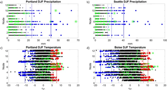
Figure 10 shows scatterplots for precipitation in Portland, Oregon, and Seattle, Washington, and Tmax
FIG. 8. Percent of extreme cold days occurring during each node in each DJF SOM node. Only grid cells determined to be statistically significant at the 5% confidence level according to a Monte Carlo simulation are shaded.
and Tmin for Portland and Boise, Idaho. Thexaxis is daily accumulated precipitation for precipitation and temperature anomaly for Tmax and Tmin with theyaxis indicating the node assignment for each day. The winter of 2015/16 was record wet in Portland and Seattle and anomalously warm across the NWUS. While not in-cluded in the SOM input, the LSMPs for each day in DJF 2015/16 were assigned to the node with the smallest RMSD. This single season is then included inFig. 10
(green symbols) to explore the efficacy of using node patterns based on historical data to inform on future local-scale temperature and precipitation extremes. Further interpretation of the anomalous 2015/16 winter is provided in the discussion insection 5.
Portland and Seattle both show strong precipitation associations with node assignment. N1, N5, N6, N9, and N10 are most frequently associated with the heaviest precipitation days in Portland and Seattle with N11 also being associated with extreme precipitation for Seattle. N5 and N6 stand out as having the strongest extreme precipitation associations, both of which are the char-acteristic AR patterns in the SOM (Fig. 3). N9 and N10, while dominated by surface high pressure, have SLP gradients conducive to strong onshore flow and a strong
250-hPa jet promoting heavy precipitation at both cities. A ridge inhibits precipitation in Portland but is sup-pressed southward enough to allow heavy precipitation in Seattle in N11. N2, N7, N8, and N12 are not strongly associated with heavy precipitation at both cities. Days assigned to these nodes tend to be associated with dry winds from the continent and/or upper-level ridging.
For temperature at Portland, N3, N4, and N8 stand out as having the most extreme cold for Tmin and N5, N6, N7, and N11 show the strongest association with extreme warmth. Here, extreme warmth can occur as a result of warm air advection from the south and west (N5 and N6) but also from winds with an easterly trajectory, which tend to be dry, thus inhibiting clouds, and can experience downslope adiabatic warming (N11 and N12). For Boise, extreme cold can occur with many synoptic regimes; however, N3, N4, and N8 stand out as having the most extreme cold. This is likely due to the ability of temper-atures to drop to extreme levels under ideal radiational cooling conditions, which can occur under multiple syn-optic conditions that allow for clear skies and calm winds. N1, N2, N5, and N6 have the strongest associations with extreme warmth, all associated with large-scale SLP gradient-induced warm air advection from the south. The
larger deviations from the mean for cold Tmin anomalies compared with warm anomalies indicate a negatively skewed temperature distribution for Boise (skewness of20.9).
b. JJA
1) SOMRESULTS AND MEAN CLIMATE ASSOCIATIONS
Figure 11shows the SOM node patterns for JJA. The main variation between nodes in SLP is the strength and position of the offshore high pressure. The surface high is strongest in the upper part of the SOM, becoming weaker toward the bottom and to the left where N9 has an offshore low. While node-to-node variations in sur-face features are mostly subtle, there is a broader range of Z500 and Z250 ridges and troughs. The left (right) side of the SOM tends to be associated with synoptic-scale troughs (ridges). N9 has a deep Z500 trough axis offshore with a closed low west of British Columbia and a strong 250-hPa jet, together with the SLP low in-dicative of a midlatitude cyclone. N11 and N2 are the most common with 12% and 11% of days, respectively, and N9 is the least common with 5.4% of days. The relatively uncommon occurrence of days assigned to N9,
which resembles stormy conditions and differs consid-erably from the climatological means in Fig. 2, corre-sponds to the relatively low rate of midlatitude cyclone passages during summer.
Composites of Tmax and insolation anomalies con-current with days assigned to each node are shown in
Fig. 12. Tmax is presented for JJA, as compared with Tmin or DJF, because summer temperature impacts are more associated with extreme heat than cold, the peaks of which are captured by the daytime high. Insolation is provided because of the strong relationship between solar heating and temperature; however, inland areas climatologically receive few clouds in JJA, resulting in small insolation anomalies there for any given node. In general, nodes toward the bottom and right are warmer than nodes to the top left. SOM corners are nearly op-posites with temperature patterns transitioning di-agonally in between. N8 is the warmest pattern domainwide and is associated with strong Z500 and Z250 ridges. This pattern resembles that associated with heat waves over the Pacific Northwest (Bumbaco et al. 2013;Brewer et al. 2012;Brewer and Mass 2016), which result primarily from clear skies and subsidence under the Z500 ridge and an inland extension of the offshore high resulting in offshore surface winds. The SLP
FIG. 10. Scatterplots of daily precipitation amount plotted according to the node that day was assigned to for (a) Portland, Oregon, and (b) Seattle, Washington. For precipitation, blue dots indicate days above the 90th percentile of the daily precipitation frequency distribution, with the first vertical blue line from left indicating the 90th, the second the 95th, and the third the 99th percentiles. Dot size increases proportionally to threshold ex-ceedance. Scatterplots for temperature are plotted for (c) Portland, Oregon, and (d) Boise, Idaho. Tmin is plotted with squares and Tmax with diamonds. Blue symbols indicate extreme cold Tmin days and red diamonds extreme warm Tmax days. The innermost blue (red) vertical lines indicate the 10th (90th) percentiles followed by the 5th (95th) and 1st (99th) percentiles moving outward. Symbol size increases proportional to anomaly magnitude. Days from DJF 2015/16 are plotted with a green asterisk.
feature is less obvious in the SOM results compared with the upper levels. Figure 13 shows positive insolation anomalies for N8 indicating maximized solar heating.
A key feature associated with heat waves across the NWUS is the thermal trough. This mesoscale feature is
usually oriented from south to north, most often along the coast or on the windward side of the Cascades, with inland occurrences also common (Brewer et al. 2012). This feature is not apparent in the SLP field of N8 or any node associated with anomalous warmth inFig. 11a. The absence of this key feature likely results from two pri-mary reasons. First, the occurrence of thermal troughs is relatively rare in any given portion of the domain, so the compositing used to createFig. 11may average out these mesoscale features. Second,Brewer et al. (2012)found that thermal troughs evolve throughout the day so the daily averages used to construct the SOM may not re-solve thermal troughs robustly. However, the large-scale Z500 ridge and subtle eastward extension of the SLP high, particularly in N4 and N8, are consistent with previous findings (e.g., Brewer et al. 2012; Bumbaco et al. 2013;Brewer and Mass 2016) supporting the SOMs approach as robust in capturing key synoptic features associated with anomalous heat in the region.
N1, N2, and N5 are associated with anomalously cool conditions domain wide. All three nodes show Z500 and Z250 troughs. Figure 13 shows negative insolation anomalies indicating increased cloud cover is a driver of the cool anomalies. N9 shows cool (warm) anomalies in the western (eastern) half of the domain. This is the node most associated with stormy conditions with on-shore winds (not shown) and strong negative insolation anomalies advecting cool marine air and diminishing solar heating. N3 has a cold north–warm south pattern broadly consistent with the placement of the 250-hPa jet position with cooler (warmer) air to the north (south) of the jet axis. N12 shows anomalous warmth toward the west, associated with a SLP gradient perpendicular to the coast promoting winds with a northerly trajectory that inhibit cool onshore flow and marine clouds from penetrating inland, as well as a Z500 ridge.
2) EXTREMES
Figure 14 shows the frequency of extreme warm Tmax days for each node. Several nodes are associated with significant occurrences of extreme warmth. N7, N8, and N10 have the largest areas covered by signifi-cant association percentages; however, N12 shows high percentages along western Washington and Oregon, consistent with the composite patterns in Fig. 12. N8 accounts for the majority of remaining extreme warm days along the coast; however, N8 also has high fre-quencies of inland heat under a broad amplified upper-level ridge. N10 shows a preference for extreme heat inland corresponding to a Z500 trough axis offshore and a ridge axis along the eastern margins. Extreme heat is absent along the coast for nodes with upper-level troughs (N1, N2, N5, and N6) and inland when
Z500 and Z250 flow is zonal (N3, N4, and N12). It is important to note that other factors that are not cap-tured by the SOMs are also important for extreme heat, such as anomalously low soil moisture anomalies (e.g.,
Berg et al. 2014;Loikith and Broccoli 2014;Seneviratne et al. 2010; Vautard et al. 2007; Fischer et al. 2007). Because precipitation extremes are generally rare and smaller in magnitude in JJA compared with DJF, do-mainwide node associations are not presented or dis-cussed in detail here.
3) LOCAL-SCALE ANALYSIS
Figure 15shows example station-scale scatterplots for JJA in the same format as Fig. 10. As noted above, precipitation is generally very light in the NWUS during the summer; however, precipitation for Spokane and Seattle is presented to demonstrate how the SOMs ap-proach can be both successful and limited at capturing precipitation extremes in the warm season. Similar to
Fig. 10for DJF 2015/16, green symbols inFig. 15indicate JJA 2015 days, a season associated with multiple warm temperature records across the NWUS. Further discus-sion on summer 2015 is provided insection 5.
Spokane (Fig. 15a), a climatologically dry city with summer average precipitation of 68 mm, shows a weak relationship between precipitation and node assign-ment. Synoptic meteorology may not be a key driver of precipitation here highlighting a limitation of the SOMs application. Additionally, precipitation is rare and generally light during the summer at Spokane with the 99th percentile of daily precipitation around 12 mm. Because a modest amount of precipitation can qualify as extreme, such events may arise out of subtle mesoscale variations in weather possible un-der multiple synoptic regimes. Seattle, conversely, exhibits relationships between node assignment and precipitation. In particular, N9 is associated with extreme summer precipitation, as are N6 and N5. The relationship with N9 and N6 is consistent with results in Fig. 15 and the midlatitude cyclone pattern in
Fig. 11.
For Portland temperature, the strongest association between node assignment and extreme warm Tmax is with N4, N8, and N12. However, these nodes are also associated with anomalous cold Tmax (not colored, and Tmax extreme cold thresholds not indicated). In
FIG. 12. Composites of JJA daily maximum temperature anomalies (K) for each SOM node. Node numbers are indicated above each panel and correspond to the node numbering convention used inFig. 11.
these cases, the broad synoptic-scale pattern may re-semble one typically associated with anomalously warm conditions, but smaller-scale features potentially relating to inland penetration of marine influence and cloud cover could cause local-scale cool anomalies. For Tmin, extreme cold can occur with multiple nodes; however, N1, N2, and N3 stand out as having relatively strong relationships with extreme cold. A relative lack of source region for extremely cold air (in an anoma-lous sense) results in apparent larger deviations from the mean on the warm side of the distribution than the cold side.
Coastal Astoria is characterized by a highly asym-metrical temperature distribution with relatively small anomalies qualifying as extreme cold Tmin and large anomalies for Tmax extremes. This highlights another limitation to the SOMs approach as applied in this pa-per, as no nodes stand out as particularly favorable for extreme temperatures, likely because temperature is highly influenced by the adjacent Pacific Ocean and subtle changes in wind direction can have major impacts on temperature locally.
5. Discussion
In this study, we demonstrate the efficacy of SOMs as a way of compactly visualizing and describing synoptic-scale weather and climate variability across the NWUS and as a basis for connecting large-scale meteorological mechanisms with local-scale extremes. This methodology has potential for application in interpreting extreme behavior in climate change pro-jections because it relies on information from spatial scales that can readily be resolved by climate models, in contrast to the more localized scales of extremes, which may not be resolved. Furthermore, by linking LSMPs with other high-impact events not well resolved or captured directly by climate models, such as lightning outbreaks, this methodology could be extended to a wide range of climate impacts. This approach may also facilitate interpretation and contextualization of the dynamics associated with very high-end extreme events (e.g.,Singh et al. 2014).
The SOMs approach offers many advantages over composite analysis for characterizing LSMPs, as outlined
FIG. 13. Composites of JJA anomalies in daily downward shortwave radiation at the surface for each SOM node, computed as fraction of the climatological mean such that a value of 1 indicates no deviation from the climatological mean. Node numbers are indicated above each panel and correspond to the node numbering convention inFig. 11.
in the introduction. Specific to climate model analysis, by using the SOMs approach, models are only required to reproduce and track changes in the node patterns and their frequencies. In contrast, composite analysis requires computing a separate composite for each location and for each type of extreme. This can result in a large number of LSMPs in need of interpretation, inhibiting systematic model evaluation and future simulation assessment.
Under future global warming, changes in extremes could result from, on the one hand, systematic changes in LSMPs, including their frequency and structure, or, on the other hand, from an overall warming of climate. In other words, change could be manifested as change in the shape of the probability density function (pdf), a shift in the pdf, or more generally a combi-nation of the two. The unusually extreme hot summer of 2015 and the warm, wet winter of 2015/16 may be viewed as consistent with expected future mean cli-mate conditions over the NWUS (Mote and Salathé 2010). While we do not claim that these anomalous seasons are the result of climate change, we consider them as case studies to illustrate how we may relate future extreme occurrence to LSMPs by posing the following question: To what extent were these seasons
characterized by unusual frequencies of LSMPs associ-ated with extremes? Here we outline the use of SOMs in answering this question as a preliminary step for the study of future climate change in subsequent research.
To determine how the daily LSMPs from the two case seasons project onto the SOMs space, we com-puted the RMSD between the SLP, Z500, and V250 from each day and each node. Days were then assigned to the node with the lowest RMSD. The multiple ex-treme precipitation events (including the greatest daily precipitation total on record at Portland) that con-tributed to the record wet winter at Portland and Seattle are apparent inFigs. 10a and 10b, respectively. For both cities, these extreme precipitation days were as-signed to nodes demonstrated by the SOMs approach to be associated with heavy precipitation over the 1979–2013 period. The frequent assignment of days to anomalously wet nodes is apparent on the rightmost bar ofFig. 7with N1, N5, N6, N8, and N9 making up 47 out of the 90 days. Winter 2015/16 was also anomalously warm across the NWUS, and node assignments reflect this for Portland and Boise inFig. 10.
Summer 2015 exhibited record warmth across the NWUS with notable occurrences of extreme temperatures
FIG. 14. As inFig. 8, but for JJA Tmax extreme warm days.
across the region. The high frequency of days with Tmax exceeding the 90th percentile is apparent inFigs. 15c,din Portland and Astoria. N2, N3, N8, N10, and N12 all had over 10 days assigned to them, and all are associated with relatively high occurrences of extreme warmth at Portland (Astoria has weaker node–temperature associations). Nodes not associated with warm temperature extremes over the western NWUS inFig. 14had few days assigned to them in summer 2015, including only one day assigned to N1 and N9. This suggests the record warmth of JJA 2015 had a large contribution from high frequencies of LSMPs that, over the historic period examined, are associated with anomalous or extreme warmth. Interestingly, many days in summer 2015 that were not extreme were also above the long-term average for both Portland and Astoria. The predominance of green symbols to the right of the zero line is notable for both cities as is the very low frequency of substantial negative Tmin anomalies. This is suggestive of an overall warmer climate during this season. Apart from secular anthropogenic warming, anomalously warm sea surface temperatures over the adjacent Pacific Ocean may have contributed to this behavior.
6. Summary and conclusions
We have applied SOMs as a tool to characterize both the winter and summer synoptic climatologies over the NWUS using daily reanalysis data and to provide a basis for physical interpretation of associated regional-and local-scale extremes in temperature regional-and precipitation. Three variables are provided as input to a 43 3 node
SOM, SLP, Z500, and V250, chosen to capture circulation near the surface and in the mid- and upper troposphere, respectively. The resultant outputs (nodes) of the SOM capture the range of synoptic regimes in the winter (Fig. 3), spanning patterns characteristic of deep midlatitude cy-clones and atmospheric rivers to strong cold inland surface high pressure systems. During summer (Fig. 11), the in-ternode variability is subtler, largely capturing variations in the persistent offshore surface high and upper-level ridges and troughs.
Composites of key surface meteorological vari-ables are constructed for days assigned to each SOM node (Figs. 4–6,12, and13). The composites indicate consistent spatial relationships between the SOM circulation patterns and surface meteorology in-cluding temperature, precipitation, and insolation. The distribution of extremes in temperature and precipitation across the nodes is generally consistent with physical expectations based on the LSMP characteristics reflected in the node patterns and the composites (Figs. 7and8for DJF andFig. 14for JJA). The SOMs approach is also demonstrated as capable of identifying patterns associated with anomalous and ex-treme temperature and precipitation days at the local or city scale with some exceptions (Figs. 10and 15). To-gether, this suggests that the SOMs approach as applied here has potential for studying changes in extremes in climate models.
Some limitations to the SOMs approach are evident. While the associations between nodes and extremes are generally robust, for some regions and some extremes
FIG. 15. As inFig. 10, but for JJA and for precipitation in (a) Spokane, Washington, and (b) Seattle, Washington, and temperature in (c) Portland, Oregon, and (d) Astoria, Oregon. Green symbols are days in JJA 2015.
there is not a clear node association. It is possible that a larger SOM array could constrain extreme days to more representative nodes in some cases; however, increas-ing the number of nodes comes at the expense of split-ting the characteristic LSMPs into smaller subgroups, restricting concise interpretation of synoptic regimes in relation to local-scale extremes. In other cases, synoptic circulation may not be the most important mechanism for extremes. For example, inland regions during winter often have low frequencies of extreme cold occurrences over multiple nodes, suggesting such extremes occur across multiple synoptic regimes (e.g., as a result of nighttime clear-sky radiative cooling). Along the coast in JJA, subtle variations in local circulation that inhibit marine influences over land can result in extreme warmth, and such variability is not well captured at the scales analyzed here. It is also possible that different combinations of quantities other than those provided as input to the SOM may improve the efficacy of the ap-proach in some cases.
Our interest in demonstrating the efficacy of using SOMs to describe the LSMPs associated with extremes in temperature and precipitation across the NWUS is motivated by the desire to better understand future changes in extremes at scales not readily resolvable by most climate models. By connecting extremes at var-ious scales to the driving LSMPs, it is possible to evaluate the ability of climate models to simulate conditions conducive to such extremes even if the models cannot directly resolve relevant impact scales. This is a topic of ongoing and future research. Fur-thermore, the LSMPs defined from SOMs provide a basis for assessing future changes in dynamical mechanisms that provide favorable conditions for extremes. Last, this methodology could be extended to other high-impact phenomena such as wildfire, lightning outbreaks, or drought.
Acknowledgments.PCL and AS acknowledge partial support from a Portland State University Faculty En-hancement Grant, and BRL acknowledges partial sup-port of New Jersey Agricultural Experiment Station Hatch Grant NJ07134. We thank Nathaniel Johnson for providing the SOMs code.
REFERENCES
Abatzoglou, J. T., 2013: Development of gridded surface meteo-rological data for ecological applications and modelling.Int. J. Climatol.,33, 121–131, doi:10.1002/joc.3413.
Anderson, S., and Coauthors, 2015: Climate action plan: Local strategies to address climate change. Portland and Multnomah County Rep., 162 pp. [Available online at https://www. portlandoregon.gov/bps/article/531984.]
Arritt, R. W., and M. Rummukainen, 2011: Challenges in regional-scale climate modeling.Bull. Amer. Meteor. Soc.,92, 365–368, doi:10.1175/2010BAMS2971.1.
Berg, A., B. R. Lintner, K. L. Findell, S. Malyshev, P. C. Loikith, and P. Gentine, 2014: Impact of soil moisture–atmosphere interactions on surface temperature distribution.J. Climate,
27, 7976–7993, doi:10.1175/JCLI-D-13-00591.1.
Brewer, M. C., and C. F. Mass, 2016: Projected changes in western U.S. large-scale summer synoptic circulations and variability in CMIP5 models. J. Climate, 29, 5965–5978, doi:10.1175/ JCLI-D-15-0598.1.
——, ——, and B. E. Potter, 2012: The West Coast thermal trough: Climatology and synoptic evolution.Mon. Wea. Rev., 140, 3820–3843, doi:10.1175/MWR-D-12-00078.1.
Bumbaco, K. A., K. D. Dello, and N. A. Bond, 2013: History of Pacific Northwest heat waves: Synoptic pattern and trends.
J. Appl. Meteor. Climatol., 52, 1618–1631, doi:10.1175/ JAMC-D-12-094.1.
Casola, J. H., and J. M. Wallace, 2007: Identifying weather regimes in the wintertime 500-hpa geopotential height field for the Pacific– North American sector using a limited-contour clustering tech-nique.J. Appl. Meteor.,46, 1619–1630, doi:10.1175/JAM2564.1. Cassano, E. N., J. M. Glisan, J. J. Cassano, J. Gutowski, and M. W.
Seefeldt, 2015: Self-organizing map analysis of widespread temperature extremes in Alaska and Canada.Climate Res.,62, 199–218, doi:10.3354/cr01274.
Cassano, J. J., P. Uotila, and A. Lynch, 2006: Changes in synoptic weather patterns in the polar regions in the twentieth and twenty-first centuries, part 1: Arctic.Int. J. Climatol.,26, 1027– 1049, doi:10.1002/joc.1306.
——, E. N. Cassano, M. W. Seefeldt, J. Gutowski, and J. M. Glisan, 2016: Synoptic conditions during wintertime temperature ex-tremes in Alaska.J. Geophys. Res. Atmos.,121, 3241–3262, doi:10.1002/2015JD024404.
Dacre, H. F., P. A. Clark, O. Martinez-Alvarado, M. A. Stringer, and D. A. Lavers, 2015: How do atmospheric rivers form?
Bull. Amer. Meteor. Soc., 96, 1243–1255, doi:10.1175/ BAMS-D-14-00031.1.
DeAngelis, A. M., A. J. Broccoli, and S. G. Decker, 2013: A comparison of CMIP3 simulations of precipitation over North America with observations: Daily statistics and circulation features accompanying extreme events.J. Climate,26, 3209– 3230, doi:10.1175/JCLI-D-12-00374.1.
Dole, R., and Coauthors, 2011: Was there a basis for anticipating the 2010 Russian heat wave?Geophys. Res. Lett.,38, L06702, doi:10.1029/2010GL046582.
Fischer, E. M., S. I. Seneviratne, P. L. Vidale, D. Luthi, and C. Schar, 2007: Soil moisture–atmosphere interactions during the 2003 European summer heat wave.J. Climate,20, 5081– 5099, doi:10.1175/JCLI4288.1.
Flato, G., and Coauthors, 2013: Evaluation of climate models.Climate Change 2013: The Physical Science Basis, T. F. Stocker et al., Eds., Cambridge University Press, 741–866.
Grotjahn, R., and Y.-Y. Lee, 2016: On climate models simula-tions of the large-scale meteorology associated with Cal-ifornia heat waves. J. Geophys. Res. Atmos., 121, 18–32, doi:10.1002/2015JD024191.
——, and Coauthors, 2016: North American extreme tempera-ture events and related large scale meteorological pat-terns: A review of statistical methods, dynamics, modeling, and trends. Climate Dyn., 46, 1151–1184, doi:10.1007/ s00382-015-2638-6.
Gutowski, W. J., and Coauthors, 2010: Regional extreme mon-thly precipitation simulated by NARCCAP RCMs.J. Hy-drometeor.,11, 1373–1379, doi:10.1175/2010JHM1297.1. Hewitson, B. C., and R. G. Crane, 2002: Self-organizing maps:
Applications to synoptic climatology.Climate Res.,22, 13–26, doi:10.3354/cr022013.
Horton, D. E., N. C. Johnson, D. Singh, D. L. Swain, B. Rajaratnam, and N. S. Diffenbaugh, 2015: Contribution of changes in atmo-spheric circulation patterns to extreme temperature trends. Na-ture,522, 465–469, doi:10.1038/nature14550.
IPCC, 2013:Climate Change 2013: The Physical Science Basis. Cambridge University Press, 1535 pp., doi:10.1017/ CBO9781107415324.
Johnson, N. C., and S. B. Feldstein, 2010: The continuum of North Pacific sea level pressure patterns: Intraseasonal, interannual, and interdecadal variability. J. Climate, 23, 851–867, doi:10.1175/2009JCLI3099.1.
——, ——, and B. Tremblay, 2008: The continuum of Northern Hemisphere teleconnection patterns and a description of the NAO shift with the use of self-organizing maps.J. Climate,21, 6354–6371, doi:10.1175/2008JCLI2380.1.
Kawazoe, S., and W. J. Gutowski, 2013: Regional, very heavy daily precipitation in NARCCAP simulations.J. Hydrometeor.,14, 1212–1227, doi:10.1175/JHM-D-12-068.1.
Lau, N.-C., and M. J. Nath, 2012: A model study of heat waves over North America: Meteorological aspects and projections for the twenty-first century.J. Climate,25, 4761–4784, doi:10.1175/ JCLI-D-11-00575.1.
——, and ——, 2014: Model simulation and projection of Euro-pean heat waves in present-day and future climates.J. Climate,
27, 3713–3730, doi:10.1175/JCLI-D-13-00284.1.
Lennard, C., and G. Hegerl, 2015: Relating changes in synoptic circulation to the surface rainfall response using self-organising maps. Climate Dyn., 44, 861–879, doi:10.1007/ s00382-014-2169-6.
Liu, Y., and R. H. Weisberg, 2011: A review of self-organizing map applications in meteorology and oceanography.Self-Organizing Maps: Applications and Novel Algorithm Design, J. I. Mwasiagi, Ed., InTech, 253–272.
Loikith, P. C., and A. J. Broccoli, 2012: Characteristics of observed atmospheric circulation patterns associated with temperature extremes over North America. J. Climate, 25, 7266–7281, doi:10.1175/JCLI-D-11-00709.1.
——, and ——, 2014: The influence of recurrent modes of climate variability on the occurrence of winter and summer extreme temperatures over North America.J. Climate,27, 1600–1618, doi:10.1175/JCLI-D-13-00068.1.
——, and ——, 2015: Comparison between observed and model-simulated atmospheric circulation patterns associated with extreme temperature days over North America using CMIP5 historical simulations.J. Climate,28, 2063–2079, doi:10.1175/ JCLI-D-13-00544.1.
——, and J. D. Neelin, 2015: Short-tailed temperature distributions over North America and implications for future changes in extremes.
Geophys. Res. Lett.,42, 8577–8585, doi:10.1002/2015GL065602. ——, D. E. Waliser, H. Lee, J. D. Neelin, B. Lintner, S. McGinnis,
L. Mears, and J. Kim, 2015: Evaluation of large-scale meteoro-logical patterns associated with temperature extremes in the NARCCAP regional climate model simulations.Climate Dyn.,
45, 3257–3274, doi:10.1007/s00382-015-2537-x.
Meehl, G. A., and C. Tebaldi, 2004: More intense, more frequent, and longer lasting heat waves in the 21st century.Science,305, 994–997, doi:10.1126/science.1098704.
Menne, M. J., I. Durre, R. S. Vose, B. E. Gleason, and T. G. Houston, 2012: An overview of the global historical clima-tology network-daily database.J. Atmos. Oceanic Technol.,
29, 897–910, doi:10.1175/JTECH-D-11-00103.1.
Mote, P. W., and E. P. Salathé, 2010: Future climate in the Pacific northwest. Climatic Change, 102, 29–50, doi:10.1007/ s10584-010-9848-z.
Radic´, V., A. J. Cannon, B. Menounos, and G. Nayeob, 2015: Future changes in autumn atmospheric river events in British Columbia, Canada, as projected by CMIP global climate models.J. Geophys. Res. Atmos.,120, 9279–9302, doi:10.1002/2015JD023279. Reusch, D. B., R. B. Alley, and B. C. Hewitson, 2005: Relative
performance of self-organizing maps and principal component analysis in pattern extraction from synthetic climatological data.Polar Geogr.,29, 188–212, doi:10.1080/789610199. Rienecker, M. M., and Coauthors, 2011: MERRA: NASA’s
Modern-Era Retrospective Analysis for Research and Applications.
J. Climate,24, 3624–3648, doi:10.1175/JCLI-D-11-00015.1. Robertson, A. W., and M. Ghil, 1999: Large-scale weather regimes
and local climate over the western United States. J. Cli-mate,12, 1796–1813, doi:10.1175/1520-0442(1999)012,1796: LSWRAL.2.0.CO;2.
Ropelewski, C. F., and M. S. Halpert, 1986: North American precipitation and temperature patterns associated with the El Nino/Southern Oscillation (ENSO). Mon. Wea. Rev.,114, 2352–2362, doi:10.1175/1520-0493(1986)114,2352: NAPATP.2.0.CO;2.
Ruff, T. W., and J. D. Neelin, 2012: Long tails in regional surface temperature probability distributions with implications for extremes under global warming. Geophys. Res. Lett., 39, L04704, doi:10.1029/2011GL050610.
Ryoo, J.-M., D. E. Waliser, D. W. Waugh, S. Wong, E. J. Fetzer, and I. Fung, 2015: Classification of atmospheric river events on the U.S. West Coast using a trajectory model.J. Geophys. Res. Atmos.,120, 3007–3028, doi:10.1002/2014JD022023. Seneviratne, S. I., T. Corti, E. L. Davin, M. Hirschi, E. B. Jaeger,
I. Lehner, B. Orlowsky, and A. J. Teuling, 2010: Investigating soil moisture–climate interactions in a changing climate: A review. Earth Sci. Rev., 99, 125–161, doi:10.1016/ j.earscirev.2010.02.004.
——, and Coauthors, 2012: Changes in climate extremes and their impacts on the natural physical environment.Managing the Risks of Extreme Events and Disasters to Advance Climate Change Adaptation, C. B. Field et al., Eds., Cambridge Uni-versity Press, 109–230.
Sheridan, S. C., and C. C. Lee, 2011: The self-organizing map in synoptic climatological research.Prog. Phys. Geogr.,35, 109– 119, doi:10.1177/0309133310397582.
Singh, D., and Coauthors, 2014: Severe precipitation in northern India in June 2013: Causes, historical context, and change in probability [in ‘‘Explaining Extreme Events of 2013’’].Bull. Amer. Meteor. Soc.,95(9), S58–S61.
Sobie, S. R., and A. J. Weaver, 2012: Downscaling of precipi-tation over Vancouver Island using a synoptic typing approach. Atmos.–Ocean, 50, 176–196, doi:10.1080/ 07055900.2011.641908.
Vautard, R., and Coauthors, 2007: Summertime European heat and drought waves induced by wintertime Mediterranean rainfall def-icit.Geophys. Res. Lett.,34, L07711, doi:10.1029/2006GL028001. Walton, D. B., F. Sun, A. Hall, and S. Capps, 2015: A hybrid
dynamical–statistical downscaling technique. Part I: Devel-opment and validation of the technique.J. Climate,28, 4597– 4617, doi:10.1175/JCLI-D-14-00196.1.