Energy Technology Systems Analysis Programme
http://www.etsap.org/tools.htm
Documentation for the TIMES Model
PART I
April 2005
Authors:
Richard Loulou
Uwe Remne
Amit Kanudia
Antti Lehtila
Gary Goldstein
General Introduction
This documentation is composed of thee Parts.
Part I comprises eight chapters constituting a general description of the TIMES
paradigm, with emphasis on the model’s general structure and its economic significance. Part I also includes a simplified mathematical formulation of TIMES, a chapter
comparing it to the MARKAL model, pointing to similarities and differences, and chapters describing new model options.
Part II is a comprehensive reference manual intended for the technically minded modeler
or programmer looking for an in-depth understanding of the complete model details, in particular the relationship between the input data and the model mathematics, or contemplating making changes to the model’s equations. Part II includes a full description of the sets, attributes, variables, and equations of the TIMES model.
Part III describes the GAMS control statements required to run the TIMES model.
GAMS is a modeling language that translates a TIMES database into the Linear Programming matrix, and then submits this LP to an optimizer and generates the result files. In addition to the GAMS program, two model interfaces (FE and VEDA-BE) are used to create, browse, and modify the input data, and to explore and further process the model’s results. The two VEDA interfaces are described in detail in their own user’s guides.
PART I: TIMES CONCEPTS AND
THEORY
TABLE OF CONTENTS FOR PART I
1 Introduction to the TIMES model 7
1.1 A brief summary ... 7
1.2 Using the TIMES model... 7
1.2.1 The Demand Component of a TIMES scenario... 8
1.2.2 The Supply Component of a TIMES Scenario ... 9
1.2.3 The Policy Component of a TIMES Scenario ... 9
1.2.4 The Techno-economic component of a TIMES Scenario... 9
2 The basic structure of the TIMES model 11 2.1 Time horizon... 13
2.2 Decoupling of data and model horizon ... 13
2.3 The RES concept... 14
2.4 Overview of the TIMES attributes ... 16
2.4.1 Parameters associated with processes... 16
2.4.2 Parameters associated with commodities... 17
2.4.3 Parameters attached to commodity flows into and out of processes... 18
2.4.4 Parameters attached to the entire RES... 18
2.5 Process and Commodity classification... 18
3 Economic rationale of the TIMES modeling approach 20 3.1. A brief classification of energy models... 20
3.1.1 ‘Top-Down’ Models ... 20
3.1.2 ‘Bottom-Up’ Models ... 21
3.1.3 Recent Modeling Advances... 22
3.2 The TIMES paradigm ... 23
3.2.1 A technology explicit model... 24
3.2.2 Multi-regional feature... 24
3.2.3 Partial equilibrium properties ... 24
3.2.3.1 Linearity... 25
3.2.3.2 Maximization of total surplus: Price equals Marginal value... 26
3.2.3.3 Competitive energy markets with perfect foresight ... 30
3.2.3.4 Marginal value pricing ... 31
3.2.3.5 Profit maximization: the Invisible Hand ... 32
4 A simplified description of the TIMES optimization program 34 4.1 Indices ... 34
4.2 Decision Variables ... 34
4.3 TIMES objective function: discounted total system cost ... 36
4.4 Constraints ... 38
4.4.1 Capacity Transfer (conservation of investments) ... 38
4.4.3 Use of capacity ... 40
4.4.4 Commodity Balance Equation:... 41
4.4.5 Defining flow relationships in a process... 42
4.4.6 Limiting flow shares in flexible processes... 43
4.4.7 Peaking Reserve Constraint (time-sliced commodities only) ... 43
4.4.8 Constraints on commodities ... 45
4.4.9 User Constraints ... 46
4.4.10 Representation of oil refining in MARKAL... 46
4.4.10.1 New sets and parameters... 46
4.4.10.2 New variables... 47
4.4.10.3 New blending constraints... 47
4.5 Linear Programming complements ... 48
4.5.1 A brief primer on Linear Programming and Duality Theory... 48
4.5.1.1 Basic definitions... 48
4.5.1.2 Duality Theory ... 49
4.5.2 Sensitivity analysis and the economic interpretation of dual variables ... 50
4.5.2.1 Economic Interpretation of the Dual Variables... 50
4.5.2.2 Reduced Surplus and Reduced Cost... 50
5 A comparison of the TIMES and MARKAL models 52 5.1 Similarities ... 52
5.2 TIMES features not in MARKAL ... 52
5.2.1 Variable length time periods... 52
5.2.2 Data decoupling... 52
5.2.3 Flexible time slices and storage processes... 53
5.2.4 Process generality ... 53
5.2.5 Flexible processes... 53
5.2.6 Investment and dismantling lead-times and costs... 54
5.2.7 Vintaged processes and age-dependent parameters ... 54
5.2.8 Commodity related variables... 55
5.2.9 More accurate and realistic depiction of investment cost payments... 55
5.2.10 Climate equations... 55
5.3 MARKAL features not in TIMES ... 56
6 Elastic demands and the computation of the supply-demand equilibrium 57 6.1 Theoretical considerations: the Equivalence Theorem ... 57
6.2 Mathematics of the TIMES equilibrium... 58
6.2.1 Defining demand functions... 58
6.2.2 Formulating the TIMES equilibrium ... 58
6.2.3 Linearization of the Mathematical Program ... 59
6.2.4 Calibration of the demand functions... 61
6.2.5 Computational considerations ... 61
6.2.6 Interpreting TIMES costs, surplus, and prices... 62
7 The Lumpy Investment option 63 7.1 Formulation and Solution of the Mixed Integer Linear Program ... 63
7.2 Important remark on the MIP dual solution (shadow prices) ... 64
8 Endogenous Technological Learning (ETL) 66 8.1 The basic ETL challenge ... 66
8.2 The TIMES formulation of ETL... 67
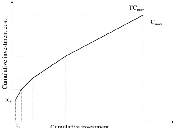
8.2.1 The Cumulative Investment Cost ... 67
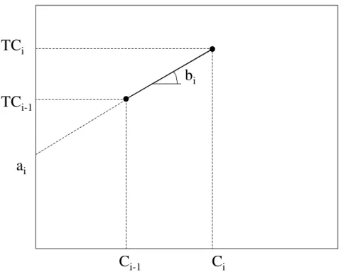
8.2.2 Calculation of break points and segment lengths... 69
8.2.3 New variables ... 70
8.2.4 New constraints ... 70
8.2.5 Objective function terms... 71
8.2.6 Additional (optional) constraints ... 71
8.3 Clustered learning... 72
8.4 Learning in a Multiregional TIMES Model... 73
1
Introduction to the TIMES model
1.1
A brief summary
TIMES (an acronym for The Integrated MARKAL-EFOM1 System) is an economic model generator for local, national or multi-regional energy systems, which provides a technology-rich basis for estimating energy dynamics over a long-term, multi-period time horizon. It is usually applied to the analysis of the entire energy sector, but may also applied to study in detail single sectors (e.g. the electricity and district heat sector).
Reference case estimates of end-use energy service demands (e.g., car road travel; residential lighting; steam heat requirements in the paper industry; etc.) are provided by the user for each region. In addition, the user provides estimates of the existing stock of energy related equipment in all sectors, and the characteristics of available future technologies, as well as present and future sources of primary energy supply and their potentials.
Using these as inputs, the TIMES model aims to supply energy services at minimum global cost (more accurately at minimum loss of surplus) by simultaneously making equipment investment and operating, primary energy supply, and energy trade decisions, by region. For example, if there is an increase in residential lighting energy service relative to the reference scenario (perhaps due to a decline in the cost of residential lighting, or due to a different assumption on GDP growth), either existing generation equipment must be used more intensively or new – possibly more efficient – equipment must be installed. The choice by the model of the generation equipment (type and fuel) is based on the analysis of the characteristics of alternative generation technologies, on the economics of the energy supply, and on environmental criteria.TIMES is thus a
vertically integrated model of the entire extended energy system.
The scope of the model extends beyond purely energy oriented issues, to the representation of environmental emissions, and perhaps materials, related to the energy system. In addition, the model is admirably suited to the analysis of
energy-environmental policies, which may be represented with accuracy thanks to the explicitness of the representation of technologies and fuels in all sectors.
In TIMES – like in its MARKAL forebear – the quantities and prices of the various commodities are in equilibrium, i.e. their prices and quantities in each time period are such that the suppliers produce exactly the quantities demanded by the consumers. This equilibrium has the property that the total surplus is maximized.
1.2
Using the TIMES model
The TIMES model is particularly suited to the exploration of possible energy futures based on contrasted scenarios. Given the long horizons simulated with TIMES, the
1 MARKAL (MARket ALlocation model, Fishbone et al, 1981, 1983, Berger et al. 1992) and EFOM (Van
scenario approach is really the only choice (whereas for the shorter term, econometric methods may provide useful projections). Scenarios, unlike forecasts, do not pre-suppose knowledge of the main drivers of the energy system. Instead, a scenario consists of a set of coherent assumptions about the future trajectories of these drivers, leading to a coherent organization of the system under study. A scenario builder must therefore carefully test the assumptions made for internal coherence, via a credible storyline. In TIMES, a complete scenario consists of four types of inputs: energy service demands, primary resource potentials, a policy setting, and the descriptions of a set of technologies. We now present a few comments on each of these four components.
1.2.1 The Demand Component of a TIMES scenario
In the case of the TIMES model demand drivers (population, GDP, family units, etc.) are obtained externally, via other models or from accepted other sources. As one example, the TIMES global model constructed for the EFDA2 used the GEM-E33 general equilibrium model to generate a set of coherent (total and sectoral) GDP growth rates in the various regions. Note that GEM-E3 itself uses other drivers as inputs in order to derive GDP trajectories. These GEM-E3 drivers consist of measures of technological progress, population, degree of market competitiveness, and a few other perhaps qualitative assumptions. For population and household projections, both GEM-E3 and TIMES used the same exogenous sources (IPCC, Nakicenovic 2000, Moomaw and Moreira, 2001). Other approaches may be used to derive TIMES drivers, whether via models or other means.
For the EFDA model, the main drivers were: Population, GDP, GDP per capita, number of households, and sector GDP. For sectoral TIMES models, the demand drivers may be different depending on the system boundaries.
Once the drivers for a TIMES model are determined and quantified the construction of the reference demand scenario requires computing a set of energy service demands over the horizon. This is done by choosing elasticities of demands to their respective drivers, in each region, using the following general formula:
Elasticity
Driver Demand =
As mentioned above, the demands are provided for the reference scenario. However, when the model is run for alternate scenarios (for instance for an emission constrained case, or for a set of alternate technological assumptions), it is likely that the demands will be affected. TIMES has the capability of estimating the response of the demands to the changing conditions of an alternate scenario. To do this, the model requires still another set of inputs, namely the assumed elasticities of the demands to their own prices. TIMES
2 EFDA: European Fusion Development Agreement
is then able to endogenously adjust the demands to the alternate cases without exogenous intervention. In fact, the TIMES model is driven not by demands but by demand curves. To summarize: the TIMES demand scenario components consist in a set of assumptions on the drivers (GDP, population, households) and on the elasticities of the demands to the drivers and to their own prices.
1.2.2 The Supply Component of a TIMES Scenario
The second constituent of a scenario is a set of supply curves for primary energy and material resources. Multi-stepped supply curves can be easily modeled in TIMES, each step representing a certain potential of the resource available at a particular cost. In some cases, the potential may be expressed as a cumulative potential over the model horizon (e.g. reserves of gas, crude oil, etc), as a cumulative potential over the ressource base (e.g. available areas for wind converters differentiated by velocities, available farmland for biocrops, roof areas for PV installations) and in others as an annual potential (e.g. maximum extraction rates, or for renewable resources the available wind, biomass, or hydro potentials). Note that the supply component also includes the identification of trading possibilities, where the amounts and prices of the traded commodities are determined endogenously (within any imposed limits).
1.2.3 The Policy Component of a TIMES Scenario
Insofar as some policies impact on the energy system, they may become an integral part of the scenario definition. For instance, a No-Policy scenario may perfectly ignore emissions of various pollutants, while alternate policy scenarios may enforce emission restrictions, or emission taxes, etc. The detailed technological nature of TIMES allows the simulation of a wide variety of both micro measures (e.g. technology portfolios, or targeted subsidies to groups of technologies), and broader policy targets (such as general carbon tax, or permit trading system on air contaminants). A simpler example might be a nuclear policy that limits the future capacity nuclear plants. Another example might be the imposition of fuel taxes, or of industrial subsidies, etc.
1.2.4 The Techno-economic component of a TIMES Scenario
The fourth and last constituent of a scenario is the set of technical and economic
parameters assumed for the transformation of primary resources into energy services. In TIMES, these techno-economic parameters are described in the form of technologies (or processes) that transform some commodities into others (fuels, materials, energy services, emissions). In TIMES, some technologies may be imposed and others may simply be available for the model to choose. The quality of a TIMES model rests on a rich, well developed set of technologies, both current and future, for the model to choose from. The emphasis put on the technological database is one of the main distinguishing factors of the class of Bottom-up models, to which TIMES belongs. Other classes of models will tend to emphasize other aspects of the system (e.g. interactions with the rest of the
economy) and treat the technical system in a more succinct manner via aggregate production functions.
Remark: two scenarios may differ in all or in only some of their components. For instance, the same demand scenario may very well lead to multiple scenarios by varying the primary resource potentials and/or technologies and/or policies, insofar as the alternative scenario assumptions do not alter the basic demand inputs (Drivers and Elasticities). The scenario builder must always be careful about the overall coherence of the various assumptions made on the four components of a scenario.
Organization of PART I
Chapter 2 provides a general overview of the representation in TIMES of the Reference Energy System (RES) of a typical region or country, focusing on its basic elements, namely technologies and commodities. Chapter 3 discusses the economic rationale of the model, and Chapter 4 presents a streamlined representation of the Linear Programming problem used by TIMES to compute the equilibrium. Chapter 5 contains a comparison of the respective features of TIMES and MARKAL, intended primarily for users already familiar with MARKAL, while Chapter 6 describes in detail the elastic demand feature and other economic and mathematical properties of the TIMES equilibrium. Chapters 7 and 8, respectively describe two model options: Lumpy Investments (LI), and Endogenous Technological Learning (ETL).
2
The basic structure of the TIMES model
It is useful to distinguish between a model’s structure and a particular instance of its implementation. A model’s structure exemplifies its fundamental approach for
representing and analyzing a problem—it does not change from one implementation to the next. All TIMES models exploit an identical mathematical structure. However, because TIMES is data4 driven, each (regional) model will vary according to the data inputs. For example, in a multi-region model one region may, as a matter of user data input, have undiscovered domestic oil reserves. Accordingly, TIMES generates
technologies and processes that account for the cost of discovery and field development. If, alternatively, user supplied data indicate that a region does not have undiscovered oil reserves no such technologies and processes would be included in the representation of that region’s Reference Energy System (RES, see sections 2.3 and 2.4). Due to this property TIMES can also be called a model generator that, based on the input information provided by the modeler, generates an instance of a model. In the following, if not stated otherwise, the expression model is used with two meanings: the instance of a TIMES model or more generally the model generator TIMES.
The structure of TIMES is ultimately defined by variables and equations determined from the data input provided by the user. This information collectively defines each TIMES regional model database, and therefore the resulting mathematical representation of the RES for each region. The database itself contains both qualitative and quantitative data. The qualitative data includes, for example, lists of energy carriers, the technologies that the modeler feels are applicable (to each region) over a specified time horizon, as well as the environmental emissions that are to be tracked. This information may be further classified into subgroups, for example energy carriers may be split by type (e.g., fossil, nuclear, renewable, etc). Quantitative data, in contrast, contains the technological and economic parameter assumptions specific to each technology, region, and time period. When constructing multi-region models it is often the case that a technology may be available for use in two distinct regions; however, cost and performance assumptions may be quite different (i.e., consider a residential heat pump in Canada versus the same piece of equipment in China). This chapter discusses both qualitative and quantitative assumptions in the TIMES modeling system.
The TIMES energy economy is made up of producers and consumers of commodities such as energy carriers, materials, energy services, and emissions. TIMES, like most equilibrium models, assumes competitive markets for all commodities. The result is a supply-demand equilibrium that maximizes the net total surplus (i.e. the sum of producers’ and consumers’ surpluses) as will be fully discussed in chapters 3 and 6. TIMES may, however, depart from perfectly competitive market assumptions by the introduction of user-defined explicit constraints, such as limits to technological
penetration, constraints on emissions, exogenous oil price, etc. Market imperfections can also be introduced in the form of taxes, subsidies and hurdle rates.
4 Data in this context refers to parameter assumptions, technology characteristics, projections of energy
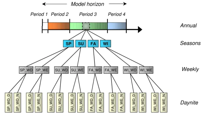
Operationally, a TIMES run configures the energy system (of a set of regions) over a certain timehorizon in such a way as to minimize the net total cost (or equivalently maximize the net total surplus) of the system, while satisfying a number of constraints. TIMES is run in a dynamic manner, which is to say that all investment decisions are made in each period with full knowledge of future events.The model is said to have perfect foresight (or to be clairvoyant). In addition to time-periods (which may be of variable length), there are time divisions within a year, also called time-slices, which may be defined at will by the user (see Figure 2.1). For instance, the user may want to define seasons, day/night, and/or weekdays/weekends. Time-slices are especially important whenever the mode and cost of production of an energy carrier at different times of the year are significantly different. This is the case for instance when the demand for an energy form fluctuates across the year and a variety of technologies may be chosen for its production. The production technologies may themselves have different characteristics depending on the time of year (e.g. wind turbines or run-of-the-river hydro plants). In such cases, the matching of supply and demand requires that the activities of the technologies producing and consuming the commodity be tracked at each time slice. Examples of commodities requiring time-slicing may include electricity, district heat, natural gas, industrial steam, and hydrogen. Two additional reasons for defining sub yearly time slices are a) the fact that the commodity is expensive (or even impossible) to store (thus requiring that production technologies be suitably activated in each time slice to match the demand), and b) the existence of an expensive infrastructure whose capacity should be sufficient to bear the peak demand for the commodity. The net result of these chracteristics is that the deployment in time of the various production technologies may be very different in different time-slices, and furthermore that specific investment decisions be taken to insure adequate reserve capacity at peak.
Model horizon Period 4 Period 3 Period 2 Period 1 Seasons Weekly Daynite WI SP SU FA
SP_WD SP_WE SU_WD SU_WE FA_WD FA_WE WI_WD WI_WE
S U _W E _N S U _W E _D S U _W D _N S U _W D _D S P _W E _N S P _W E _D S P _W D _N S P _W D _D W I_ W E _N W I_ W E _D W I_ W D _N W I_ W D _D FA _W E _N FA _W E _D FA _W D _N FA _W D _D Annual
2.1
Time horizon
Thetime horizon is divided into a (user-chosen) number of time-periods, each model period containing a (possibly different) number of years. For TIMES each year in a given period is considered identical, except for the cost objective function which differentiates between payments in each year of a period. For all other quantities
(capacities, commodity flows, operating levels, etc) any model input or output related to period t applies to each of the years in that period, with the exception of investment variables, which are usually made only once in a period5,. In this respect, TIMES is similar to MARKAL but differs from the approach used in EFOM, where capacities and flows were assumed to evolve linearly between so-called milestone years.
The initial period is usually considered a past period, over which the model has no freedom, and for which the quantities of interest are all fixed by the user at their historical values. It is often advised to choose an initial period consisting of a single year, in order to facilitate calibration to standard energy statistics. Calibration to the initial period is one of the more important tasks required when setting up a TIMES model. The main
variables to be calibrated are: the capacities and operating levels of all technologies, as well as the extracted, exported, imported, produced, and consumed quantities for all energy carriers, and the emissions if modeled.
In TIMES years preceding the first period also play a role. Although no explicit variables are defined for these years, data may be provided by the modeler on past investments. Note carefully that the specification of past investments influences not only the initial period’s calibration, but also the model’s behavior over several future periods, since the past investments provide residual capacity in several years within the modeling horizon proper.
2.2
Decoupling of data and model horizon
In TIMES, special efforts have been made to de-couple the specification of data from the definition of the time periods for which a model is run. Two TIMES features facilitate this decoupling.
First, the fact that investments made in past years are recognized by TIMES makes it much easier to modify the choice of the initial and subsequent periods without major revisions of the database.
Second, the specification of process and demand input data in TIMES is made by specifying the years when the data apply, and the model takes care of interpolating and extrapolating the data to represent the particular periods chosen by the modeler for a particular model run.
5 There are exceptional cases when an investment must be repeated more than once in a period, namely
when the period is so long that it exceeds the technical life of the investment. These cases are described in detail in section 5.2 of PART II.
These two features combine to make a change in the definition of periods quite easy and error-free. For instance, if a modeler decides to change the initial year from 1995 to 2005, and perhaps change the number and durations of all other periods as well, only one type of data change is needed, namely to define the investments made from 1995 to 2004 as past investments. All other data specifications need not be altered6. This feature
represents a great simplification of the modeler’s work. In particular, it enables the user to define time periods that have varying lengths, without changing the input data.
2.3
The RES concept
The TIMES energy economy consists of three types of entities:
Technologies (also called processes) are representations of physical devices that transform commodities into other commodities. Processes may be primary sources of commodities (e.g. mining processes, import processes), or transformation activities such as conversion plants that produce electricity, energy-processing plants such as refineries, end-use demand devices such as cars and heating systems, etc,
Commodities consisting of energy carriers, energy services, materials, monetary flows, and emissions. A commodity is generally produced by some process(es) and/or consumed by other process(es), and
Commodity flows, that are the links between processes and commodities. A flow is of the same nature as a commodity but is attached to a particular process, and represents one input or one output of that process.
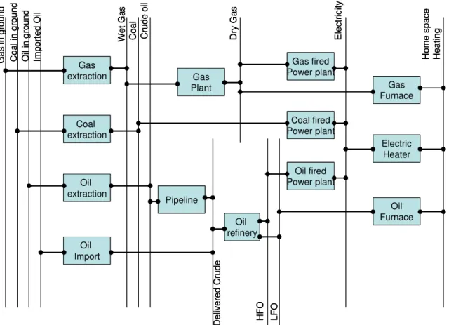
It is helpful to picture the relationships among these various entities using a network diagram, referred to as a Reference Energy System (RES). In TIMES, the RES processes are represented as boxes and commodities as vertical lines. Commodity flows are
represented as links between process boxes and commodity lines. Using graph theory terminology, a RES is an oriented graph, where both the processes and the commodities are the nodes of the graph. They are interconnected by the flows, which are the arcs of the graph. Each arc (flow) is oriented and links exactly one process node with one commodity node. Such a graph is called bi-partite, since its set of nodes may be
partitioned into two subsets and there are no arcs directly linking two nodes in the same subset.
Figure 2.2 depicts a small portion of a hypothetical RES containing a single energy service demand, namely residential space heating. There are three end-use space heating technologies using the gas, electricity, and heating oil energy carriers (commodities), respectively. These energy carriers in turn are produced by other technologies,
represented in the diagram by one gas plant, three electricity-generating plants (gas fired, coal fired, oil fired), and one oil refinery. To complete the production chain on the primary energy side, the diagram also represents an extraction source for natural gas, an
6 However, if the horizon has been lengthened, additional data for the new years at the end of the horizon
extraction source for coal, and two sources of crude oil (one extracted domestically and then transported by pipeline, and the other one imported). This simple RES has a total of 13 commodities and 13 processes. These elements form Note that in the RES every time a commodity enters/leaves a process (via a particular flow) its name is changed (e.g., wet gas becomes dry gas, crude becomes pipeline crude). This simple rule enables the inter-connections between the processes to be properly maintained throughout the network.
Figure 2.2. Partial view of a simple Reference Energy System (all arcs are oriented left to right)
To organize the RES, and inform the modeling system of the nature of its components, the various technologies, commodities, and flows may be classified into sets. Each TIMES set regroups components of a similar nature. The entities belonging to a set are referred to as members, items or elements of that set. The same item may appear in multiple technology or commodity sets. While the topology of the RES can be
represented by a multi-dimensional network, which maps the flow of the commodities to the various technologies, the set membership conveys the nature of the individual
components and is often most relevant to post-processing (reporting) than influencing the model structure itself.
Gas extraction Coal extraction Oil extraction Oil Import Gas fired Power plant Coal fired Power plant Oil fired Power plant Oil refinery Gas Plant Pipeline Oil Furnace Electric Heater Gas Furnace G as in g ro un d C oa l i n gr ou nd O il in g ro un d Im po rte d O il D el iv er ed C ru de D ry G as C oa l W et G as C ru de o il LF O H FO E le ct ric ity H om e sp ac e H ea tin g Gas extraction Coal extraction Oil extraction Oil Import Gas fired Power plant Coal fired Power plant Oil fired Power plant Oil refinery Gas Plant Pipeline Oil Furnace Electric Heater Gas Furnace G as in g ro un d C oa l i n gr ou nd O il in g ro un d Im po rte d O il D el iv er ed C ru de D ry G as C oa l W et G as C ru de o il LF O H FO E le ct ric ity H om e sp ac e H ea tin g
Contrary to MARKAL, TIMES has relatively few sets for forming process or commodity groups. In MARKAL the processes are differentiated depending on whether they are sources, conversion processes, end-use devices, etc., and processes in each set have their own specialized attributes. In TIMES most processes are endowed with essentially the same attributes (with the exceptions of storage and inter-regional exchange processes), and unless the user decides otherwise (e.g. by providing values for some attributes and ignoring others), they have the same variables attached to them, and must obey similar constraints. Therefore, the differentiation between the various species of processes or commodities is made through data specification only, thus eliminating the need to define specialized membership sets (unless desired for processing results). Most of the TIMES features (e.g. sub-annual time-slice resolution, vintaging) are available for all processes and the modeler chooses the features being assigned to a particular process by specifying a corresponding indicator set (e.g. PRC_TSL, PRC_VINT).
However, the TIMES commodities are still classified into several Major Groups. There are five such groups: energy carriers, materials, energy services, emissions, and monetary flows. The use of these groups is essential in the definition of some TIMES constraints, as discussed in chapter 4.
2.4
Overview of the TIMES attributes
TIMES has some attributes that were not available in MARKAL. More importantly, some attributes correspond to powerful new features that confer to TIMES additional flexibility. The complete list of attributes is shown in PART II, and we provide below only succinct comments on the types of attribute attached to each entity of the RES or to the RES as a whole.
Attributes may be cardinal (e.g. numbers) or ordinal (e.g. sets). For example, some of ordinal attributes are defined for process to describe subsets of flows that are then used to construct specific flow constraints. Subsection 4.4 describes such flow constraints,a nd Chapter 2 of PART II gives the complete list of TIMES sets.
The cardinal attributes are usually called parameters. We give below a brief idea of the types of parameters available in the TIMES model generator.
2.4.1 Parameters associated with processes
TIMES process-oriented parameters fall into three general categories. First are technical parameters that include efficiency, availability factor(s), commodity consumptions per unit of activity, shares of fuels per unit activity, technical life of the process, construction lead time, dismantling lead-time and duration, amounts of the commodities consumed (respectively released) by the construction (respectively dismantling) of one unit of the process, and contribution to the peak equations. The efficiency, availability factors, and
commodity inputs and outputs of a process may be defined in several flexible ways depending on the desired process flexibility, on the time-slice resolution chosen for the process and on the time-slice resolution of the commodities involved. Certain parameters are only relevant to special processes, such as storage processes or processes that
implement trade between regions.
The other class of process parameters is economic and policy parameters that include a variety of costs attached to the investment, dismantling, maintenance, and operation of a process. In addition, taxes and subsidies may be defined in a very flexible manner. Other economic parameters are the economic life of a process (which is the time during which the investment cost of a process is amortized, which may differ from the operational lifetime) and the process specific discount rate, also called hurdle rate, both of which serve to calculate the annualized payments on the process investment cost.
Finally, the modeler may impose a variety of bounds (upper, lower, equality) on the investment, capacity, and activity of a process.
Note that many process parameters may be vintaged (i.e. dependent upon the date of installation of new capacity), and furthermore may be defined as being dependent on the age of the technology. The latter feature is implemented by means of special data
grouped under the SHAPE parameter, which introduces user-defined shaping indexes that can be applied to age-dependent parameters. For instance, the annual maintenance cost of an automobile could be defined to remain constant for say 3 years and then increase in a linear manner each year after the third year.
2.4.2 Parameters associated with commodities
Commodity-oriented parameters fall into three categories.
Technical parameters associated with commodities include overall efficiency (for
instance grid efficiency), and the time-slices over which that commodity is to be tracked. For demand commodities, in addition the annual projected demand and load curves (if the commodity has a subannual time-slice resolution) can be specified.
Economic parameters include additional costs, taxes, and subsidies on the overall or net production of a commodity.. These cost elements are then added to all other (implicit) costs of that commodity. In the case of a demand service, additional parameters define the demand curve (i.e. the relationship between the quantity of demand and its price). These parameters are: the demand’s own-price elasticity, the total allowed range of variation of the demand value, and the number of steps to use for the discrete approximation of the curve.
Policy based parameters include bounds (at each period or cumulative) on the overall or net production of a commodity, or on the imports or exports of a commodity by a region.
In TIMES the net or the total production of each commodity may be explicitly represented by a variable, if needed for imposing a bound or a tax. No such direct possibility was available in MARKAL, although the same result could be achieved via clever modeling.
2.4.3 Parameters attached to commodity flows into and out of processes
A commodity flow (more simply, a flow) is an amount of a given commodity produced or consumed by a given process. Some processes have several flows entering or leaving it, perhaps of different types (fuels, materials, demands, or emissions). In TIMES, unlike in MARKAL, each flow has a variable attached to it, as well as several attributes
(parameters or sets)
Technical parameters (along with some set attributes), permit full control over the maximum and/or minimum share a given input or output flow may take within the same commodity group. For instance, a flexible turbine may accept oil or gas as input, and the modeler may use a parameter to limit the share of oil to at most 40% of the total fuel input. Other parameters and sets define the amount of certain outflows in relation to certain inflows (e.g., efficiency, emission rate by fuel). For instance, in an oil refinery a parameter may be used to set the total amount of refined products equal to 92% of the total amount of crude oils (s) entering the refinery, or to calculate certain emissions as a fixed proportion of the amount of oil consumed. If a flow has a sub-annual time-slice resolution, a load curve can be specified for the flow7.
Economic parameters include delivery and other variable costs, taxes and subsidies attached to an individual process flow.
2.4.4 Parameters attached to the entire RES
These parameters include currency conversion factors (in a multi-regional model), region-specific time-slice definitions, a region-specific general discount rate, and reference year for calculating the discounted total cost (objective function). In addition, certain switches control the activation of the data interpolation procedure as well as special model features to be employed (e.g., run with ETL, see chapter 8).
2.5
Process and Commodity classification
Although TIMES does not explicitly differentiate processes or commodities that belong to different portions of the RES (with the exception of storage and trading processes), there are three ways in which some differentiation does occur.
7 It is possible to define not only load curves for a flow, but also bounds on the share of a flow in a specific
time-slice relative to the annual flow, e.g. the flow in the time-slice “WinterDay” has to be at least 10 % of the total annual flow.
First, TIMES does require the definition of Primary Commodity Groups (pcg), i.e. subsets of commodities of the same nature entering or leaving a process. For each given process, the modeler defines a pcg as a subset of commodities of the same nature, eitehr entering or leaving the process as flows. TIMES uses the pcg to define the activity of the process, and also its capacity. Besides establishing the process activity and capacity, these groups are convenient aids for defining certain complex quantities related to process flows, as discussed in section 4.4 and in PART II.
As noted previously TIMES does not require that the user provide many set
memberships. However, the TIMES report step does pass some set declarations to the VEDA-BE result-processing system to facilitate construction of results analysis tables. These include process subsets to distinguish demand devices, energy processes, material processes (by weight or volume), refineries, electric production plants, coupled heat and power plants, heating plants, storage technologies and distribution (link) technologies; and commodity subsets for energy, useful energy demands (split into six aggregate sub-sectors), environmental indicators, and materials.
The third instance of commodity or process differentiation is not embedded in TIMES, but rests on the modeler. A modeler may well want to choose process and commodity names in a judicious manner so as to more easily identify them when browsing through the input database or when examining results. As an example, the World Multi-regional TIMES model developed within ETSAP adopts a naming convention whereby the first three characters denote the sector and the next three the fuel (e.g., light fuel oil used in the residential sector is denoted RESLFO). Similarly, process names are chosen so as to identify the sub-sector or end-use (first three characters), the main fuel used (next three), and the specific technology (last four). For instance, a standard (001) residential water heater (RHW) using electricity (ELC) is named RWHELC001. Naming conventions may thus play a critical role in allowing the easy identification of an element’s position in the RES.
Similarly, energy services may be labeled so that they are more easily recognized. For instance, the first letter may indicate the broad sector (e.g. ‘T’ for transports) and the second letter designate any homogenous sub-sectors (e.g. ‘R’ for road transport), the third character being free.
In the same fashion, fuels, materials, and emissions are identified so as to immediately designate the sector and sub-sector where they are produced or consumed. To achieve this some fuels have to change names when they change sectors, which is accomplished via processes whose primary role is to change the name of a fuel. In addition, such a process may serve as a bearer of sector wide parameters such as distribution cost, price markup, tax, that are specific to that sector and fuel. For instance, a tax may be levied on industrial distillate use but not on agricultural distillate use, even though the two
commodities are physically identical.
3
Economic rationale of the TIMES modeling approach
This chapter provides a detailed economic interpretation of the TIMES and other partial equilibrium models based on maximizing total surplus. Partial equilibrium models have one common feature – they simultaneously configure the production and consumption of commodities (i.e. fuels, materials, and energy services) and their prices. The price of producing a commodity affects the demand for that commodity, while at the same time the demand affects the commodity’s price. A market is said to have reached an
equilibrium at prices p* and quantities q* when no consumer wishes to purchase less than q* and no producer wishes to produce more than q* at price p*. Both p* and q* are vectors whose dimension is equal to the number of different commodities being modeled. As will be explained below, when all markets are in equilibrium the total economic surplus is maximized.
The concept of total surplus maximization extends the direct cost minimization approach upon which earlier bottom-up energy system models were based. These simpler models had fixed energy service demands, and thus were limited to minimizing the cost of supplying these demands. In contrast, the TIMES demands for energy services are themselves elastic to their own prices, thus allowing the model to compute a bona fide supply-demand equilibrium. This feature is a fundamental step toward capturing the main feedback from the economy to the energy system.
Section 3.1 provides a brief review of different types of energy models. Section 3.2 discusses the economic rationale of the TIMES model with emphasis on the features that distinguish TIMES from other bottom-up models (such as the early incarnations of MARKAL, see Fishbone and Abilock, 1981, Berger et al., 1992, though MARKAL has since been extended beyond these early versions). Section 3.3 describes the details of how price elastic demands are modeled in TIMES, and section 3.4 provides additional discussion of the economic properties of the model.
3.1.
A brief classification of energy models
Many energy models are in current use around the world, each designed to emphasize a particular facet of interest. Differences include: economic rationale, level of
disaggregation of the variables, time horizon over which decisions are made (and which is closely related to the type of decisions,i.e. only operational planning or also investment decisions), and geographic scope. One of the most significant differentiating features among energy models is the degree of detail with which commodities and technologies are represented, which will guide our classification of models in two major classes.
3.1.1 ‘Top-Down’ Models
At one end of the spectrum are aggregated General Equilibrium (GE) models. In these each sector is represented by a production function designed to simulate the potential substitutions between the main factors of production (also highly aggregated into a few variables such as: energy, capital, and labor) in the production of each sector’s output. In this model category are found a number of models of national or global energy systems.
These models are usually called “Top-Down”, because they represent an entire economy via a relatively small number of aggregate variables and equations. In these models, production function parameters are calculated for each sector such that inputs and outputs reproduce a single base historical year.8 In policy runs, the mix of inputs9 required to produce one unit of a sector’s output is allowed to vary according to user-selected elasticities of substitution. Sectoral production functions most typically have the following general form:
(
ρ ρ ρ)
1/ρ0 K s L S E S
s A B K B L B E
X = ⋅ + ⋅ + ⋅ (3-1)
where XS is the output of sector S,
KS, LS, and ES are the inputs of capital, labor and energy needed to produce one unit of output in sector S,
is the elasticity of substitution parameter,
A0 and theB’s are scaling coefficients.
The choice of determines the ease or difficulty with which one production factor may be substituted for another: the smaller is (but still greater than or equal to 1), the easier it is to substitute the factors to produce the same amount of output from sector S. Also note that the degree of factor substitutability does not vary among the factors of production — the ease with which capital can be substituted for labor is equal to the ease with which capital can be substituted for energy, while maintaining the same level of output. GE models may also use alternate forms of production function (3-1), but retain the basic idea of an explicit substitutability of production factors.
3.1.2 ‘Bottom-Up’ Models
At the other end of the spectrum are the very detailed, technology explicit models that focus primarily on the energy sector of an economy. In these models, each important energy-using technology is identified by a detailed description of its inputs, outputs, unit costs, and several other technical and economic characteristics. In these so-called
‘Bottom-Up’ models, a sector is constituted by a (usually large) number of logically arranged technologies, linked together by their inputs and outputs (commodities, which may be energy forms or carriers, materials, emissions and/or demand services). Some bottom-up models compute a partial equilibrium via maximization of the total net (consumer and producer) surplus, while others simulate other types of behavior by economic agents, as will be discussed below. In bottom-up models, one unit of sectoral output (e.g., a billion vehicle kilometers, one billion tonnes transported by heavy trucks or one Petajoule of residential cooling service) is produced using a mix of individual technologies’ outputs. Thus the production function of a sector is implicitly constructed,
8 These models assume that the relationships (as defined by the form of the production functions as well as
the calculated parameters) between sector level inputs and outputs are in equilibrium in the base year.
9 Most models use inputs such as labor, energy, and capital, but other input factors may conceivably be
added, such as arable land, water, or even technical know-how. Similarly, labor may be further subdivided into several categories.
rather than explicitly specified as in more aggregated models. Such implicit production functions may be quite complex, depending on the complexity of the reference energy system of each sector (sub-RES).
3.1.3 Recent Modeling Advances
While the above dichotomy applied fairly well to earlier models, these distinctions now tend to be somewhat blurred by recent advances in both categories of model. In the case of aggregate top-down models, several general equilibrium models now include a fair amount of fuel and technology disaggregation in the key energy producing sectors (for instance: electricity production, oil and gas supply). This is the case with MERGE10 and
SGM11, for instance. In the other direction, the more advanced bottom-up models are ‘reaching up’ to capture some of the effects of the entire economy on the energy system. For instance, the TIMES model has end-use demands (including demands for industrial output) that are sensitive to their own prices, and thus capture the impact of rising energy prices on economic output and vice versa. Recent incarnations of technology-rich models are multi-regional, and thus are able to consider the impacts of energy-related decisions on trade. It is worth noting that while the multi-regional top-down models have always represented trade, they have done so with a very limited set of traded commodities – typically one or two, whereas there may be quite a number of traded energy forms and materials in multi-regional bottom-up models.
MARKAL-MACRO (see [9]) is a hybrid model combining the technological detail of MARKAL with a succinct representation of the macro-economy consisting of a single producing sector. Because of its succinct single-sector production function, MARKAL-MACRO is able to compute a general equilibrium in a single optimization step. The NEMS12 model is another example of a full linkage between several technology rich modules of the various energy subsectors and a set of macro-economic equations, although the linkage here is not as tight as in MARKAL-MACRO, and thus requires iterative resolution methods.
The TIMES model introduces further enhancements over and above those of MARKAL. In TIMES, the horizon may be divided into periods of unequal lengths, thus permitting a more flexible modeling of long horizons: typically, one may adopt short periods in the near-term (the initial period often consists of a single base year), and longer ones in the out years; TIMES includes both technology related variables (as in MARKAL) and flow related variables (as in the EFOM model,van der Voort et. al., 1984), thus allowing the easy creation of more flexible processes and constraints; the expression of the TIMES objective function (total system cost) tracks the payments of investments and other costs much more precisely that in other bottom-up models; and, several other new features of TIMES that are fully discussed in chapters 4 and 5, and in PART II of this
documentation.
10 Model for Evaluating Regional and Global Effects (Manne et al., 1995) 11 Second Generation Model (Edmonds et al., 1991)
12 National Energy Modeling System, a detailed integrated equilibrium model of an energy system linked to
In spite of these advances in both classes of models, there remain important differences. Specifically:
• Top-down models encompass macroeconomic variables beyond the energy sector proper, such as wages, consumption, and interest rates, and
• Bottom-up models have a rich representation of the variety of technologies (existing and/or future) available to meet energy needs, and, they often have the capability to track a wide variety of traded commodities.
The Top-down vs. Bottom-up approach is not the only relevant difference among energy models. Among Top-down models, the so-called Computable General
Equilibrium models (CGE) described above differ markedly from the macro econometric models. The latter do not compute equilibrium solutions, but rather simulate the flows of capital and other monetized quantities between sectors (see e.g. Meade, 1996 on the LIFT model). They use econometrically derived input-output coefficients to compute the impacts of these flows on the main sectoral indicators, including economic output (GDP) and other variables (labor, investments). The sectoral variables are then aggregated into national indicators of consumption, interest rate, GDP, labor, and wages.
Among technology explicit models also, two main classes are usually distinguished: the first class is that of the partial equilibrium models such as MARKAL and TIMES, that use optimization techniques to compute a least cost (or maximum surplus) path for the energy system. The second class is that of simulation models, where the emphasis is on representing a system not governed purely by financial costs and profits. In these simulation models (e.g. CIMS, Jaccard et al. 2003), investment decisions taken by a representative agent (firm or consumer) are only partially based on profit maximization, and technologies may capture a share of the market even though their life-cycle cost may be higher than that of other technologies. Simulation models use market-sharing formulas that preclude the easy computation of equilibrium – at least not in a single pass. The SAGE incarnation of the MARKAL model possesses a market sharing mechanism that allows it to reproduce certain behavioral characteristics of observed markets.
The next section focuses on the TIMES model, the most recent advanced partial equilibrium model.
3.2
The TIMES paradigm
Since certain portions of this and the next sections require an understanding of the concepts and terminology of Linear Programming, the reader requiring a brush-up on this topic may first read section 4.5, and then, if needed, some standard textbook on LP, such as Hillier and Lieberman (1990) or Chvàtal (1983). The application of Linear
Programming to microeconomic theory is covered in Gale (1960), and in Dorfman, Samuelson, and Solow (1958, and subsequent editions).
A brief description of TIMES would express that it is a:
• Technology explicit;
• Partial equilibrium model; that assumes:
• Price elastic demands; and
• Competitive markets: with
• Perfect foresight (resulting in Marginal value Pricing) We now proceed to flesh out each of these properties.
3.2.1 A technology explicit model
As already presented in chapter 2 (and described in much more detail in Part II), each technology is described in TIMES by a number of technical and economic parameters. Thus each technology is explicitly identified (given a unique name) and distinguished from all others in the model. A mature TIMES model may include several thousand technologies in all sectors of the energy system (energy procurement, conversion, processing, transmission, and end-uses) in each region. Thus TIMES is not only technology explicit, it is technology rich as well. Furthermore, the number of
technologies and their relative topology may be changed at will, purely via data input specification, without the user ever having to modify the model’s equations. The model is thus to a large extent data driven.
3.2.2 Multi-regional feature
Some existing TIMES models covering the entire energy system include up to 15 regional modules, while some existing sectoral models consist of up to 27 regions. The number of regions in a model is limited only by the difficulty of solving LP’s of very large size. The individual regional modules are linked by energy and material trading variables, and by emission permit trading variables, if desired. The trade variables transform the set of regional modules into a single multi-regional (possibly global)
energy model, where actions taken in one region may affect all other regions. This feature is of course essential when global as well as regional energy and emission policies are being simulated. Thus a multi-regional TIMES modeled is geographically integrated.
3.2.3 Partial equilibrium properties
TIMES computes a partial equilibrium on energy markets. This means that the model computes both the flows of energy forms and materials as well as their prices, in such a way that, at the prices computed by the model, the suppliers of energy produce exactly the amounts that the consumers are willing to buy. This equilibrium feature is present at every stage of the energy system: primary energy forms, secondary energy forms, and energy services. A supply-demand equilibrium model has as economic rationale the maximization of the total surplus, defined as the sum of suppliers and consumers
particular mathematical properties of the model. In TIMES, these properties are as follows:
• Outputs of a technology are linear functions of its inputs (subsection 3.2.3.1);
• Total economic surplus is maximized over the entire horizon (3.2.3.2), and
• Energy markets are competitive, with perfect foresight (3.2.3.3). As a result of these assumptions the following additional properties hold:
• The market price of each commodity is equal to its marginal value in the overall system (3.2.3.4), and
• Each economic agent maximizes its own profit or utility (3.2.3.5). .
3.2.3.1 Linearity
A linear input-to-output relationship first means that each technology represented may be implemented at any capacity, from zero to some upper limit, without economies or diseconomies of scale. In a real economy, a given technology is usually available in discrete sizes, rather than on a continuum. In particular, for some real life technologies, there may be a minimum size below which the technology cannot be implemented (or else at a prohibitive cost), as for instance a nuclear power plant, or a hydroelectric
project. In such cases, because TIMES assumes that all technologies may be implemented in any size, it may happen that the model’s solution shows some technology’s capacity at an unrealistically small size. However, in most applications, such a situation is relatively infrequent and often innocuous, since the scope of application is at the country or
region’s level, and thus large enough so that small capacities are unlikely to occur. On the other hand, there may be situations where plant size matters, for instance when the region being modeled is very small. In such cases, it is possible to enforce a rule by which certain capacities are allowed only in multiples of a given size (e.g., build or not a gas pipeline), by introducing integer variables. This option, referred to as Lumpy
Investment (LI) is available in TIMES and is discussed in chapter 7. This approach should, however, be used sparingly because it greatly increases solution time.
Alternatively and more simply, a user may add user-defined constraints to force to zero any capacities that are clearly too small.
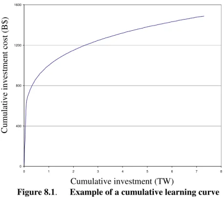
It is the linearity property that allows the TIMES equilibrium to be computed using Linear Programming techniques. In the case where economies of scale or some other non-convex relationship is important to the problem being investigated, the optimization program would no longer be linear or even convex. We shall examine such a case in chapter 8 when discussing Endogenous Technology Learning.
The fact that TIMES’s equations are linear, however, does not mean that production functions behave in a linear fashion. Indeed, the TIMES production functions are usually highly non-linear (although convex), representing non-linear functions as a stepped sequence of linear functions. As a simple example, a supply of some resource may be represented as a sequence of segments, each with rising (but constant within its interval) unit cost. The modeler defines the ‘width’ of each interval so that the resulting supply
curve may simulate any non-linear convex function. In brief, diseconomies of scale are usually present at the sectoral level.
3.2.3.2 Maximization of total surplus: Price equals Marginal value
The total surplus of an economy is the sum of the suppliers’ and the consumers’ surpluses. The term supplier designates any economic agent that produces (and sells) one or more commodities (i.e., in TIMES, an energy form, a material, an emission permit, and/or an energy service). A consumer is a buyer of one or more commodities. In TIMES, the suppliers of a commodity are technologies that procure a given commodity, and the consumers of a commodity are technologies or demands that consume a given commodity. Some technologies may be both suppliers and consumers, but not of the same commodity (since a technology never has the same commodity as input and output, with the exception of storage technologies13). Therefore, for each commodity the RES defines a set of suppliers and a set of consumers.
It is customary in microeconomics to represent the set of suppliers of a commodity by their inverse production function, that plots the marginal production cost of the
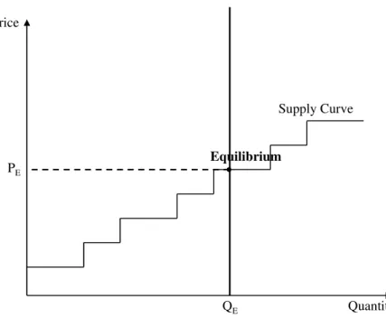
commodity (vertical axis) as a function of the quantity supplied (horizontal axis). In TIMES, as in other linear optimization models, the supply curve of a commodity is not explicitly expressed as a function of aggregate factor inputs such as capital, labor and energy (as they would in typical production functions used in the economic literature). However, it is a standard result of Linear Programming theory that the inverse supply function is step-wise constant and increasing in each factor (see Figures 2 and 3. for the case of a single commodity14). Each horizontal step of the inverse supply function
indicates that the commodity is produced by a certain technology or set of technologies in a strictly linear fashion. As the quantity produced increases, one or more resources in the mix (either a technological potential or some resource’s availability) is exhausted, and therefore the system must start using a different (more expensive) technology or set of technologies in order to produce additional units of the commodity, albeit at higher unit cost. Thus, each change in production mix generates one step of the staircase production function with a value higher than the preceding step. The width of any particular step depends upon the technological potential and/or resource availability associated with the set of technologies represented by that step.
13 Even here, a storage process consumes a given commodity at a certain time-slice or period, and restitutes
it at a later time-slice or period. Therefore, the output commodity is not identical to the input commodity.
14 This is so because in Linear Programming the shadow price of a constraint remains constant over a
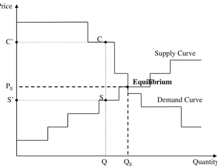
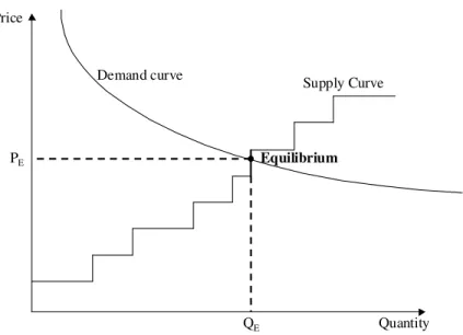
Figure 3.1. Equilibrium in the case of an energy form: the model implicitly constructs both the supply and the demand curves
In a similar manner, each TIMES instance defines a series of inverse demand
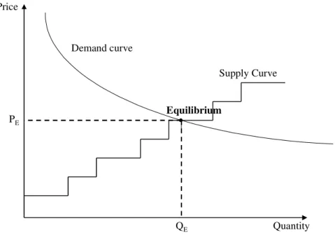
functions. In the case of demands, two cases are distinguished. First, if the commodity in question is an energy carrier whose production and consumption are endogenous to the model, then its demand function is implicitly constructed within TIMES, and is a step-wise constant, decreasing function of the quantity demanded, as illustrated in Figure 3.1 for a single commodity. If on the other hand the commodity is a demand for an energy service, then its demand curve is defined by the user via the spcification of the own-price elasticity of that demand, and the curve is in this instance a smoothly decreasing curve as illustrated in Figure 3.215. In both cases, the supply-demand equilibrium is at the
intersection of the supply function and the demand function, and corresponds to an equilibrium quantity QE and an equilibrium price PE16. At price PE, suppliers are willing
to supply the quantity QE and consumers are willing to buy exactly that same quantity QE.
Of course, the TIMES equilibrium concerns many commodities, and the equilibrium is a multi-dimensional analog of the above, where QE and PE are now vectors rather than
scalars.
The above description of the TIMES equilibrium is valid for any energy form that is entirely endogenous to TIMES, i.e. an energy carrier, material, or emission permit. In the case of an energy service, TIMES does not implicitly construct the demand function. Rather, the user explicitly defines the demand function by specifying its own price
15 This smooth curve will be discretized later for computational purposes, as described in chapter 6 16 As may be seen in figures 2 and 3, the equilibrium is not necessarily unique. In the case shown in Figure
2, any point on the vertical segment containing the equilibrium is also an equilibrium, with the same QE but
a different PE. In other cases, the multiple equilibria may have the same price and different quantities.
Price Quantity QE Supply Curve Demand Curve PE Q C’ S’ C S Equilibrium
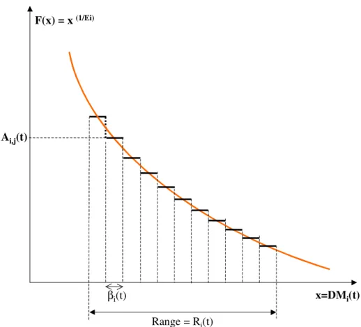
elasticity. Each energy service demand is assumed to have a constant own price elasticity function of the form (see Figure 3.2):
D/D0 = (P/P0)E (3.3-1)
Where {D0 ,P0} is a reference pair of demand and price values for that energy service over the forecast horizon, and E is the (negative) own price elasticity of that energy service demand, as chosen by the user (note that though not shown by the notation, this price elasticity may vary over time). The pair {D0, P0} is obtained by solving TIMES for a reference scenario. More precisely, D0is the demand projection estimated by the user in the reference case based upon explicitly defined relationships to economic and
demographic drivers, and P0 is the shadow price of that energy service demand obtained
by running the reference case scenario of TIMES.
Using Figure 3.1 as an example, the definition of the suppliers’ surplus corresponding to a certain point S on the inverse supply curve is the difference between the total revenue and the total cost of supplying a commodity, i.e. the gross profit. In Figure 3.1, the
surplus is thus the area between the horizontal segment SS’ and the inverse supply curve. Similarly, the consumers’ surplus for a point C on the inverse demand curve, is defined as the area between the segment CC’ and the inverse demand curve. This area is a consumer’s analog to a producer’s profit; more precisely it is the cumulative opportunity gain of all consumers who purchase the commodity at a price lower than the price they would have been willing to pay. For a given quantity Q, the total surplus (suppliers’ plus consumers’) is simply the area between the two inverse curves situated at the left of Q. It should be clear from Figure 3.1 that the total surplus is maximized exactly when Q is equal to the equilibrium quantity QE. Therefore, we may state (in the single commodity
case) the following Equivalence Principle:
“The supply-demand equilibrium is reached when the total surplus is maximized” This is a remarkably useful result, as it leads to a method for computing the equilibrium, as will be see in much detail in Chapter 6. In the multi-dimensional case, the proof of the above statement is less obvious, and requires a certain qualifying property (called the integrability property) to hold (Samuelson, 1952, Takayama and Judge, 1972). One sufficient condition for the integrability property to be satisfied is realized when the cross-price elasticities of any two energy forms are equal, viz.
j
i
Q
P
Q
P
j/
∂
i=
∂
i/
∂
jfor
all
,
∂
In the case of commodities that are energy services, these conditions are trivially satisfied in TIMES because we have assumed zero cross price elasticities. In the case of an energy carrier, where the demand curve is implicitly derived, it is also easy to show that the integrability property is always satisfied17. Thus the equivalence principle is valid in all
cases.
17 This results from the fact that in TIMES each price P
iis the shadow price of a balance constraint (see
section 4.5), and may thus be (loosely) expressed as the derivative of the objective function F with respect to the right-hand-side of a balance constraint, i.e. ∂F/∂Qi. When that price is further differentiated with
In summary, the equivalence principle guarantees that the TIMES supply-demand equilibrium maximizes total surplus.The total surplus concept has long been a mainstay of social welfare economics because it takes into account both the surpluses of consumers and of producers.18
Figure 3.2. Equilibrium in the case of an energy service: the user, explicitly provides the demand curve, usually using a simple functional form
Remark: In older versions of MARKAL, and in several other least-cost bottom-up models, energy service demands are exogenously specified by the modeler, and only the cost of supplying these energy services is minimized. Such a case is illustrated in Figure 3.3 where the “inverse demand curve” is a vertical line. The objective of such models was simply the minimization of the total cost of meeting exogenously specified levels of energy service.
respect to another quantity Qj, one gets ∂2F/∂Qi•∂Qj, which, under mild conditions is always equal
to ∂2F/∂Qj •∂Qi, as desired.
18 See e.g. Samuelson, P, and W. Nordhaus (1977)
Price Quantity QE Supply Curve PE Equilibrium Demand curve
Figure 3.3. Equilibrium when an energy service demand is fixed
3.2.3.3 Competitive energy markets with perfect foresight
Competitive energy markets are characterized by perfect information and atomic economic agents, which together preclude any of them from exercising market power. That is, neither the level any individual producer supplies, nor the level any individual consumer demands, affects the equilibrium market price (because there are many other buyers and sellers to replace them). It is a standard result of microeconomic theory that the assumption of competitive markets entails that the market price of a commodity is equal to its marginal value in the economy. This is of course also verified in the TIMES economy, as discussed in the next subsection.
In TIMES, the perfect information assumption extends to the entire planning horizon, so that each agent has perfect foresight, i.e. complete knowledge of the market’s
parameters, present and future. Hence, the equilibrium is computed by maximizing total surplus in one pass for the entire set of periods. Such a farsighted equilibrium is also called an inter-temporal,dynamic or clairvoyant equilibrium.
Note that there are at least two ways in which the perfect foresight assumption may be relaxed: in one variant, agents are assumed to have foresight over a limited portion of the horizon, say one period. Such an assumption of limited foresight is embodied in the SAGE variant of MARKAL. There is for the time being no such variant of the TIMES model. In another variant, foresight is assumed to be imperfect, meaning that agents may only assume probabilities for certain key future events. This assumption is at the basis of the Stochastic Programming option in Standard MARKAL. A Stochastic