Master’s Programme in ICT Innovation
Pei Zhang
Performance Analysis of Cloud-Based
Stream Processing Pipelines for
Real-Time Vehicle Data
Master’s Thesis Espoo, July 24, 2019
Supervisor: Professor Antti Yl¨a-J¨a¨aski, Aalto University Advisor: Cheng Xu Ph.D.Sc. (Tech.)
Master’s Programme in ICT Innovation MASTER’S THESIS Author: Pei Zhang
Title:
Performance Analysis of Cloud-Based Stream Processing Pipelines for Real-Time Vehicle Data
Date: July 24, 2019 Pages: 62
Major: EIT Digital - Cloud Computing and Services
Code: SCI3081 Supervisor: Professor Antti Yl¨a-J¨a¨aski
Advisor: Cheng Xu Ph.D.Sc. (Tech.)
The recent advancements in stream processing systems enabled applications to exploit fast-changing data and provide real-time services to companies and users. This kind of application requires high throughput and low latency to provide the most value. This thesis work, in collaboration with Scania, provides fundamental blocks for the efficient development of latency-optimized, cloud-based, real-time processing pipelines.
With investigation and analysis of the real-time Scania pipeline, this thesis deliv-ers three contributions, that can be employed to speed up the process of devel-oping, testing and optimizing low-latency streaming pipelines in many different contexts.
The first contribution is the design and implementation of a generic framework for testing and benchmarking AWS based streaming pipelines. This framework allows collecting latency statistics from every step of the pipeline. The insights it produces can be used to quickly identify bottlenecks of the pipeline.
Employing this framework, the study then proceeds to analyze the behaviour of Scania serverless streaming pipeline, which is AWS Kinesis and AWS Lambda services. The results show the importance of optimizing configuration parameters such as memory size and batch size. Several suggestions of best configurations and optimization of the pipeline are discussed.
Finally, the thesis offers a survey of the main alternatives to Scania pipeline, including Apache Spark Streaming and Apache Flink. With an analysis of the benefits and drawbacks of each framework, We choose Flink as an alternative solution. Scania pipeline is adapted to Flink with new design and implementation. Benefits of Flink pipeline and performance comparison are discussed in detail. Overall, this work can be used as an extensive guide to the design and implemen-tation of efficient, low-latency pipelines to be deployed on the cloud.
Keywords: Stream Processing, AWS, Latency, Data Pipeline, Flink Language: English
ICT-Innovation maisteriohjelma TIIVISTELM ¨A Tekij¨a: Pei Zhang
Ty¨on nimi:
Pilvipohjaisten prosessointiputkistojen suorituskykyanalyysi reaaliaikaista ajo-neuvotietoa varten
P¨aiv¨ays: 24. hein¨akuu 2019 Sivum¨a¨ar¨a: 62 P¨a¨aaine: EIT Digital - Cloud Computing
ja palvelut
Koodi: SCI3081 Valvoja: Professori Antti Yl¨a-J¨a¨aski
Ohjaaja: Cheng Xu Ph.D.Sc. (Tech.) ¨
Askett¨aiset edistykset stream-prosessointij¨arjestelmiss¨a antoivat sovelluksille mahdollisuuden hy¨odynt¨a¨a nopeasti muuttuvaa tietoa ja tarjota reaaliaikaisia palveluita yrityksille ja k¨aytt¨ajille. T¨allainen sovellus vaatii suurta suorituskyky¨a ja matalaa latenssia, jotta saadaan suurin arvo. T¨am¨a tutkielma tarjoaa yhteis-ty¨oss¨a Scanian kanssa perustavanlaatuiset lohkot latenssiin optimoitujen, pilvi-pohjaisten, reaaliaikaisten prosessointiputkien tehokkaalle kehitt¨amiselle.
Tutkimalla ja analysoimalla reaaliaikaista Scania-putkilinjaa, t¨am¨a opinn¨aytety¨o antaa kolme kommenttia, joita voidaan k¨aytt¨a¨a nopeuttamaan pienviiveisten vir-tausputkien kehitt¨amis-, testaus- ja optimointiprosessia monissa eri yhteyksiss¨a. Ensimm¨ainen ty¨o on AWS-pohjaisten suoratoistoputkien testaamista ja vertailua-nalyysej¨a koskevan yleisen kehyksen suunnittelu ja toteutus. T¨am¨a kehys mahdol-listaa latenssitilastojen ker¨a¨amisen jokaisesta vaiheesta. Sen tuottamia oivalluksia voidaan k¨aytt¨a¨a nopeasti tunnistamaan putkilinjan pullonkaulat.
T¨at¨a kehyst¨a hy¨odynt¨aen tutkimus etenee sitten Scania-palvelimettoman suora-toistoputken, joka on AWS Kinesis- ja AWS Lambda -palvelut, k¨aytt¨aytymisen analysointiin. Tulokset osoittavat konfiguraatioparametrien, kuten muistin koon ja er¨an koon, optimoinnin t¨arkeyden. Keskustetaan useista ehdotuksista parhaim-mista kokoonpanoista ja putkilinjan optimoinnista.
Lopuksi tutkielma tarjoaa tutkimuksen t¨arkeimmist¨a vaihtoehdoista Scania-putkilinjalle, mukaan lukien Apache Spark Streaming ja Apache Flink. Analy-soimalla kunkin kehyksen hy¨odyt ja haitat, valitsemme vaihtoehtoiseksi ratkai-suksi Flinkin. Scania-putkisto on mukautettu Flinkille uudella suunnittelulla ja toteutuksella. Flink-putkiston ja suorituskyvyn vertailun eduista keskustellaan yksityiskohtaisesti.
Kaiken kaikkiaan t¨at¨a ty¨ot¨a voidaan k¨aytt¨a¨a kattavana oppaana pilveen asennet-tavien tehokkaiden, pienen viiveell¨a putkistojen suunnittelussa ja toteutuksessa. Asiasanat: Virran k¨asittely, AWS, latenssi, dataputki, Flink
Kieli: Englanti
This thesis was written at Scania Group, many thanks to Scania for giving me this interesting thesis topic and all the resources I need to work on this thesis.
I would like to thank my professor Antti Yl¨a-J¨a¨aski for giving me this opportunity working on this topic and for all the suggestions and support that help me finish my thesis properly. I am grateful to have Cheng Xu as my thesis instructor who always gives me dedicated guidance and valuable feedback during the whole thesis work.
Also I would like to express my gratitude to all the members of Sca-nia ECCE department, expecially my manager Annika and CESI team for supporting my thesis work and giving me instructions.
Last, I want to thank all my friends and family for being there for me.
Espoo, July 24, 2019 Pei Zhang
AWS Amazon Web Services
CRISP CRoss Industry Standard Process
DBMS Database Processing Management System DSMS Data Stream Management System
CQ Continuous Queries protobuf Protocol Buffers
DB Database
SQL Structured Query Language CSV Comma-Separated Values Amazon KDS Amazon Kinesis Data Streams Amazon KDA Amazon Kinesis Data Analytics Amazon S3 Amazon Simple Storage Service Amazon EC2 Amazon Elastic Compute Cloud Amazon EMR Amazon Elastic MapReduce Amazon SQS Amazon Simple Queue Service RDD Resilient Distributed Dataset Async Asynchronous
Abbreviations and Acronyms 5
1 Introduction 8
1.1 Problem Statement . . . 9
1.2 Structure of the Thesis . . . 10
2 Background 12 2.1 Data Analysis . . . 12
2.2 Real-Time Stream Processing . . . 14
2.2.1 Stream Processing Architectures . . . 15
2.2.2 Continuous Query . . . 16
2.2.3 Processing Operators . . . 17
2.2.4 Windowing . . . 18
2.3 Stream Processing Systems . . . 20
2.4 Cloud Computing . . . 20
3 Current Solution 21 3.1 Background . . . 21
3.2 Amazon Web Service . . . 21
3.2.1 Amazon Kinesis Data Streams . . . 22
3.2.2 Amazon Lambda . . . 22 3.2.3 Amazon DynamoDB . . . 23 3.2.4 Amazon CloudWatch . . . 24 3.2.5 Amazon ElastiCache . . . 25 3.2.6 Amazon EMR . . . 25 3.3 Protocol Buffers . . . 26
3.4 Current Data Pipeline . . . 26
4 Benchmarking Environment 29 4.1 Motivation . . . 29
4.2 Benchmarking Design . . . 30
5 Pipeline Performance 33 5.1 Background . . . 33 5.2 Experiments . . . 34 5.3 Results Evaluation . . . 35 5.4 Latency Discussion . . . 40 6 Alternative Solution 41 6.1 Overview of Streaming Frameworks . . . 42
6.2 Comparison of Streaming Frameworks . . . 43
6.2.1 Dynamic Enrichment . . . 43 6.2.2 Internal Caching . . . 43 6.2.3 Input/Output Format . . . 44 6.2.4 Delivery Guarantees . . . 44 6.2.5 Latency . . . 45 6.2.6 Throughput . . . 45
6.3 Alternative Solution Design . . . 46
6.3.1 Overview . . . 46
6.3.2 Design Principles . . . 47
6.4 Prototype Implementation . . . 48
6.5 Result Evaluation and Discussion . . . 49
7 Discussion 50 7.1 Performance Comparison . . . 50
7.2 Future Work . . . 51
7.2.1 Improve Benchmarking Environment . . . 51
7.2.2 Current Pipeline Optimization . . . 52
7.2.3 Complete New Flink Solution . . . 53
8 Conclusions 55
A Structure of Flink Project Prototype 61
Introduction
The development of hardware technology enables a large amount of real-time data generated from a variety of devices everyday. For example, smart devices send real-time position data to map services, connected devices continuously send sensors data to monitoring or analyzing applications. These big vol-ume data comes from different sources in real-time composing data streams. Applications and services built on streaming data, on one hand, have to man-age infinite data set since data items are produced continuously; on the other hand, they require real-time processing to be able to response immediately with detecting potential failures or making right decisions. Thus, the ability to exploit fast-changing data and provide real-time services to companies and users has become the competitive advantage of service providers.
Scania is one of the world’s leading manufacturers of trucks and buses for heavy transports. Today, they have more than 400,000 connected vehicles generating a huge amount of data in real time every day. In Scania connected services and collaboration, a real-time stream processing pipeline is used to collect and process hundreds of measurements every second, collected by the smart sensors installed in modern trucks. The outputs of this streaming pipeline are used by data analysis and machine learning teams as qualified input data sources, to provide multiple different real-time services to their customers. As in real-time applications, data value vanishes gradually with time goes by. A streaming pipeline must have high throughput and low latency in order to provide the most value. Therefore, this Scania data streaming pipeline not only provides high quality of data to other data-driven services but also needs to process data in a short time period.
In order to ensure the quality of data. Scania constructs its streaming pipeline with following data pre-processing rules. In the data streaming area, data pre-processing is one of the most critical components which is used to provide good quality of data. The real-world raw data is most likely produced
with errors, out of order, and missing values. Data pre-processing transforms raw data into an understandable format as well as correcting inconsistency and incomplete. Generally, data pre-processing has several steps, including data cleaning, data integration, data transformation, data reduction, and data discretization. Considering the user cases of pre-processed data, a com-mon data pre-processing procedure has some or all the steps. Data cleaning is mainly for correcting consistency, such as data arriving time, and remov-ing empty values. Data integration is also called data enrichment, which joins multiple data sets together. Data transformation is normalizing data to make sure all the values have the same units. Data reduction and data dis-cretization are reducing the volume of data to produce similar results. Scania pipeline chooses some steps from whole data pre-processing flow to ensure data quality, which includes data enriching, data cleaning and normalizing based on real industry requirements.
When having the mechanism to keep data quality, improving the perfor-mance of the streaming pipeline becomes more and more important. High throughput and low latency are other key requirements of Scania streaming pipeline. However, there are several challenges in finding better streaming data processing solutions in terms of performance. The goal of this thesis work is to design and implement an alternative data pre-processing pipeline, and then do a performance comparison between different solutions as well as different capacity configurations, in order to find the best solution or best configuration which can achieve high throughput and low latency.
1.1
Problem Statement
Currently, Scania Connected Services has a cloud-based data pre-processing pipeline where sensor raw data is collected from each connected vehicle and then processed with other cloud services. Pre-processed data is used to feed machine learning models for further analyzing, such as, failure detection and transporting decisions making.
The goal of this thesis work is defined with considering the following questions:
1. What is the performance of current Scania streaming pipeline?
Current Scania data pre-processing pipeline has four steps: decoding, enriching, cleaning and normalizing. These four steps are connected to each other with Amazon Kinesis Data Streams (KDS) and implemented with AWS Lambda functions. The producer in this pipeline is incoming sensor data, consumers in this pipeline are each component as well as
other storage readers. The performance we need to measure here is latency and throughput. With measuring latency and throughput, its easy for us to find the bottleneck of this pipeline and what factors contribute to performance.
2. How to optimize current pipeline to achieve better performance? The capability of AWS services based systems really depends on par-ticular user cases with special configurations. For example, the number of shards in Kinesis streams affects the whole throughput this pipeline can manage. Moreover, the memory of Lambda function decides the processing time of each trigger. We need to find optimizing solutions as it is impossible to just increase shards and memory to infinite. The challenge of this optimization is that it is better to have a stable bench-marking environment which can easily tell us the different performance results with corresponding configurations.
3. Considering the requirements of current data streaming pipeline, what is the alternative solution of Scania data pre-processing pipeline? Streaming data has its own characteristics and corresponding use cases. It is important to understand how and why these data are constructed as well as data transferring between pre-processing steps. Moreover, there are many existing streaming frameworks such as Apache Spark Streaming, or from other Cloud providers, such as Google Data Flow, it is difficult to find one which is suitable for all requirements. In the end, we have to design a new solution and compare it with the current Scania pipeline to see the advantages and disadvantages of these different approaches. Furthermore, we will implement the new solution with basic features to show the performance in terms of throughput and latency.
1.2
Structure of the Thesis
The rest of this thesis is organized with following parts:
• Chapter 2 presents a background knowledge with literature review, such as data streaming systems and stream processing technologies
• Chapter 3 is an overview of developing environment, different services, tools and an in-depth view of current data pipeline
• Chapter 4 is giving the performance measurement framework with de-sign and implementation
• Chapter 5 is doing experiments of measuring performance, and analyz-ing and discussanalyz-ing the results
• Chapter 6 presents a comparison of different streaming frameworks and shows the design and implementation of the alternative solution
• Chapter 7 is comparing current Scania pipeline with new solution, dis-cussing possible optimization and future work
Background
This chapter presents the background of stream processing including what stream processing is, techniques used in data streaming and stream process-ing frameworks. As stream processprocess-ing is a particular branch of data analysis, an overview of big data analyzing is given first.
2.1
Data Analysis
Data analysis is a particular research field in big data, which applies the advanced analytic techniques into large, multi-source and diverse data sets. These datasets are high-volume, high-velocity, high-variety and requiring in-novative and cost-effective processing [25]. Data analysis has been playing an important role in the business world for a long time with helping a busi-ness operate more competitively and efficiently, such as adapting customers, making decisions and doing predictions [32]. With these given advantages, currently, more and more areas embrace data analysis in their applications, for example, public transportation in big cities, risk management in the in-surance industry, efficient delivery in logistic companies, or city planning by government [8].
The process of data analysis is obtaining raw data from real world and converting them into valuable information. The strategy used in data anal-ysis is called exploratory data analanal-ysis (EDA), which is also known as data mining as an extension. Data mining defines a group of developed exploratory techniques and methods employed for analyzing voluminous data sets [33]. In order to make independent data mining projects from different industries with various used techniques being more repeatable, more manageable and less costly, a standard process model in data mining has been developed which is CRISP-DM (CRoss Industry Standard Process for Data Mining)
[31]. This CRISP is breaking the whole data mining process into six phases with respective tasks which can be seen in Figure 2.1.
Figure 2.1: Overview of CRISP and tasks[31]
In these six stages, business understanding and data understanding are closely connected to each other, which aim to figure out the mission of data mining projects and get familiar with data characteristics. Modeling, evalu-ation and deploying work together to deliver final analyzing products. The crucial phase among these process steps is data preparation. It covers all the actions used to transform initial raw data into constructed final data which can be used to serve the next step for modeling. Since the raw data gath-ered from real world normally are out-of-range, missing values or erroneous combinations, for example, a kid with age 66. Models and applications built from these inaccurate data sets constantly have a number of different types of issues, which particularly applies the natural law ”garbage in, garbage out” [27]. That means the final analyzing is useless. Therefore, the higher the quality of prepared data is, the more accurate models can be established, the more value final products can create.
Data preparation consists of a set of operations converting low-quality raw data into properly formatted data which can perfectly feed into mining models subsequently. Techniques and methodologies employed in data pre-processing are intended to resolve problems in natural data and then provide high-quality data. As discussed in the book [22], data quality is composed of many factors, including accuracy, completeness, consistency, timeless, believ-ability and interpretbeliev-ability. For each type of data quality, data pre-processing has a specific category of techniques can be used to guarantee final results. Here we illustrate some pre-processing procedures.
Data Integration
Data integration refers to the merging of data from multiple data stores [18]. This process usually performs to enrich current data sets with external data. Typical operations include detecting missing fields in current data sets and integrating data from different sources without conflicts.
Data Cleaning
Data cleaning refers to a group of operations that filter inaccurate data, detect bad values, reduce unnecessary or duplicated data [18]. In general, data cleaning detects defects in dirty data and clean them with certain rules. For example, cleaning missing timestamps events, cleaning data items with negative value when it represents age or year. Except for errors, cleaning can also be used to remove useless data in order to reduce the data volume a little bit.
Data Normalization
Data normalization refers to unifying the measurement units of all the at-tributes in data sets. For example, normalizing all the distance-related fields to meters instead of using miles and inches. Normalizing aims to let all parameters have the same weight in the later analysis.
Noise Identification
Actually, noise identification is one step of data cleaning which helps data transformation going smoothly. Diffing from removing errors, noise identifi-cation corrects them with certain rules or concepts.
2.2
Real-Time Stream Processing
Stream processing is a technique adapted by real-time big data analyzing. It aims to process data streams without accessing the whole data items which actually are infinite and continuously arrive. A data stream refers to a group of data points generated from different sources, such as GPS data from smart-phones, IoT sensors data, and web application logs. These data points are real-time, unordered, unlimited and full of errors, and independent from each other even in the same stream [5]. However, more and more applications are built with streaming data including network traffic analysis, weblogs analysis for business recommendation and user location tracking. The value of these
applications can provide is decreasing with time goes by, which means we can-not use the traditional way to retrieve all the data, put data into databases and then process them for other usages. Furthermore, unlike static and fixed datasets, streaming data has its special characteristics, such as arriving con-tinuously, rapid increasing, potentially infinite in size and coming out of order from multiple sources. All of these make managing stream processing much harder than normal datasets and it has already pushed the limitations of using traditional database processing management systems (DBMSs).
The traditional DBMSs are designed to send a variety of queries on ex-isted data sets. It loads all the data into the database first and then does query whenever we want a result. That is, in DBMS, data is stored in persistent relational data formats that only have small or infrequently up-dates, but queries are changing based on various requirements of applications. However, a data stream management system (DSMS) works in the opposite way. In DSMS, data is moving, queries are fixed. Most DSMSs implement and store the queries with known purposes before data arrives, new data elements of streams arrive continuously to trigger these queries and then compute new results constantly over time. Instead of using large shared databases like DBMSs, stream processing only maintains part of processing data, which reduces demanding infrastructure resources. Moreover, com-pared with DBMSs, everything is fixed and static like data items, database products, in stream processing, everything is flowing. For example, the re-sults of one query cloud also be streams that can flow to another processing program as incoming streams. Thus, a data streaming system takes one or more streams of data as input and produces one or more streams of outputs, streaming data keeps flowing in and out of the system without storing any of them.
2.2.1
Stream Processing Architectures
Stream processing is a processing model that connects sequential computing tasks with data streams. A simplest stream processing architecture looks like this: in general, there are multiple sources producing data as incoming data streams, such as IoT data, weblogs, transactions. There are several con-sumers consuming or producing outgoing streams, such as databases, filesys-tems or another stream processor. Between producers and consumers, there are message brokers such as Kafka, Kinesis connecting them together, which ensures data moving from producer to consumer smoothly. In detail, there are also many computing operators between producers and consumers. Each operator takes one or more input streams and produces one or more output streams.
Logically speaking, the general processing model exposed as above makes no major differences among all DSMSs. However, internally, by adapting different ways to perform these computations can make a big difference.
The significant internal architecture consideration which has been dis-cussed in many existed studies is micro-batch processing versus one-record-at-a-time stream processing. The former consists of buffering incoming events in small batches and then perform bulk operations on these batches. It is used, for example, by Spark Streaming which benefits from leveraging the underlying extremely efficient bulk processing capabilities of the Spark en-gine. The latter, which is used, for example, by Storm and Flink, consists instead of processing one item at a time, as soon as it reaches an operator.
Another internal architecture implementation which also contributes to computation difference is parallelism. There are three kinds of parallelism: pipeline parallelism, where successive operators are scheduled on different machines, task parallelism, where independent branches of the dataflow are scheduled on different machines, and data parallelism, where the same oper-ator is scheduled on more than one machine, with the events load-balanced among them. These parallelism models are not mutually exclusive, but some of them might be more effective on some architectures than others. For example, data parallelism is a perfect match for Spark Streaming and its mini-batch approach, as it is also the underlying principle in the Spark en-gine. On the other hand, the streaming architecture of Flink, makes it better suited for pipeline parallelism [21].
2.2.2
Continuous Query
Both DBMSs and DSMSs are mainly about operating data with queries. Dif-ferent from traditional DBMS using a one-time query, data stream processing systems process streams of data with continuous queries (CQs). A continu-ous query is a query that is issued once in a data stream system and then logically continuously runs over the data in the system until it is terminated [14]. As data in DSMSs is moving with time, the results of query executions are also changing over time.
With considering the registering time of queries in DSMSs, queries are categorized into two types: predefined queries and ad-hoc queries [13]. A predefined query is created before seeing the streams of data and the value of the expected results of this query are the same every time. In contrast, an ad-hoc query is scheduled after data streams starting for a particular demand from the user. In general, an ad-hoc query is a dynamical and short-time execution. However, as ad-hoc queries require history data elements that have already been processed or discard in DSMSs, in order to answer these
queries, the system has to keep a period of time of data.
Therefore, another core concept in stream processing is having approx-imate results. An approxapprox-imate result can be done with bounded memory, limited time and incomplete data items from a stream. Compared with tradi-tional DBMSs which can always give accurate answers to queries. The ability of DSMSs to give precise answers are different, as there are some challenges coming with continuous queries processing:
• Unbounded arriving data with bounded memory and other computa-tion resources
• Processing streams of data probably needs extra statistics data or other streams
• Data streams are often burst, lost and data characteristics are varying with time
However, it is good to know that a well-behaved stream processing framework can compute approximate results almost as same as precise results.
2.2.3
Processing Operators
The process of stream data can be described as directed trees, as you can see the example in Figure 2.2. Source data is root. Final consumers or applications are leaves. In between, there are many nodes that could either be intermediate data or operators. Intermediate data can be directed to storage or other operators. Operators perform operations to transform input streaming data flow to outputs.
Figure 2.2: A Simple Dataflow Model (Source: [16])
There are two varieties of operators, stateless and stateful [28]. In the stream processing, the state represents the ability of operators to preserving
past information in memory that can be used to compute results during future processing. Stateless operations are simple functions that only use current incoming data items to perform the outputs, without complying with past knowledge or future information. Common stateless operators include map which applies to each element in a stream and returns the same amount of new elements after transformation, and filter which similar applies to each element but only returns elements that fulfill the predefined requirements. For example, if we want to add execution timestamp into each element, we can use a map operation, and if we want to retrieve items with only positive values, we can use a filter function. All in all, these operations do not rely on what they have already seen in the past and what will receive in the future. In contrast, stateful operations are functions which require operators remember data value from past event to perform the outputs. Examples are sort,average andrelational joins where the computing results are depend on history data.
2.2.4
Windowing
Windowing is one of the most important implementations in stream pro-cessing which groups infinite streaming data into smaller finite chunks. As stream processing loads all computing data into memory instead of accessing resident data from disks, the usage of memory is going to be unbounded if it stores the entire history data streams. In the previous section, we briefly introduced operators in stream processing. We know that in terms of state-less operations, including filter and map, they can be processed one by one without asking other dependencies. However, for stateful operators, such as avg, sort which require historical data, and the results are heavily related to the length of history data. For example, the average running speed in an hour is totally different from average speed in 12 hours as perhaps there are only 4 hours valid running time within these 12 hours. In this situation, a windowing configuration can let operators know that the size of data that they should maintain for each execution.
There are two main types of windows employed in the stream processing system. They are sliding windows and tumbling windows. They both store data items as they received but differ in triggers and evictions policies [19].
A tumbling window is a window storing data items with pre-defined size. Data is ready for processing when the window is full. After data processing completes, the window evicts all data in it to prepare an empty window for the next processing.
A sliding window is a window maintaining the most recent data records. A window is moving as a fixed length of the queue. When a new data item
arrives, it is put into the window, once the window is full, the oldest data elements are evicted to make up room for new arriving ones. Similar to the Tumbling window, data is ready for processing when the window is full. Unlike a tumbling window removes all data items, sliding windows evict old items for new arrives.
The eviction policies of windowing decide how and when data is being processed in the window. Both tumbling window and sliding window can be count-based, time-based and punctuation-based.
• Count-based. A count-based window is defined by the number of data tuples.
• Time-based. A time-based window is determined by a period of clock time.
• Punctuation-based. Punctuation represents boundaries in a stream which divide an infinite stream into finite pieces. Punctuation-based eviction policy is only suitable for a tumbling window, which stores all the data items until seeing a punctuation.
Operations with windowing can be a combination of window type and evic-tion policy. For example, using a count-based tumbling window to process 100 data items at a time, or using a time-based tumbling window to com-pute results with one-minute messages without counting the number of items. Similarly, it could also have a time-based sliding window or count-based slid-ing window.
In addition to time-based windowing, it has more complicated scenarios as the time here represents three different types of time:
• Event time. Event time is the logic time embedded inside the data item itself when the data item is created.
• Processing Time. The clock time when the data item is processed.
• Ingestion time. Ingestion time is the timestamp assigned when data item ingests into the data streaming system.
Event time in one given data item never changes, in contrast, processing time changes constantly when events flow through different processing proce-dures. Ingestion time is normally assigned by the streaming system which is system bound. Different streaming systems have different support for these three notions of time. For example, Flink supports all these three-time do-mains to provide a flexible way for programmers to define the correlations
among events [15]. As discussed in [6], there is a dynamically changing skew between event time and processing time. This skew represents the arbitrary delay for having processing results based on event time. Hence, some systems introduce watermark which is a global process metric to visualize this skew.
2.3
Stream Processing Systems
Stream processing has rich prior work including academic research and com-mercial applies. For example, the STREAM streaming prototype from Stan-ford [7], which aims at building a model to solve the problem that traditional databases can not be applied to real-time applications. STREAM prototype creates a bunch of queries over continuous unbounded streams. In STREAM project, they designed continuous query language (CQL) which is a con-crete declarative query language that implements streams and relations of time-based items. However, this prototype still needs several improvements to complete the project, such as STREAM is a centralized model, instead, modern applications produce distrusted data stream source.
There also exists several stream processing frameworks designed for low-latency real-time data processing. such as Apache Storm, Spark Streaming and Flink, which will be discussed in the following chapters.
2.4
Cloud Computing
Cloud computing has been widely used in hundreds and thousands of busi-nesses as it can replace a big amount of upfront infrastructure expenses into smaller various payments. United States National Institute of Standard and Technology (NIST) [26] defines cloud computing as a model which enables convenient delivery in a shared pool of computer resources such as storage, networks, databases, application services through network accessing, cus-tomers can reserve and release these resources with little management effort and a ”pay-as-you-go” price. With using cloud computing, applications can be easily developed, deployed and distributed with low costs and automati-cally scale up / down with real-time requirements.
Cloud providers like Google and Amazon, both provide cloud-based stream processing services, for example, Google Cloud Dataflow and Amazon Kine-sis. In the later chapters, we present the Amazon cloud-based stream pro-cessing solutions.
Current Solution
In this chapter, we present the company case this thesis is working on, and explain how the current stream processing system works with detailed expla-nations about used services.
3.1
Background
Scania provides transport solutions to users with a wide range of applications, which aim to help customers efficiently manage their vehicles, in the end, to improve profitability. These applications include for example real-time position tracking, driver performance coaching, and remote diagnostics which are all driven by live data collected from connected vehicles. Scania has more than 500,000 connected vehicles that send real-time data to the data processing platform everyday. With collecting and analyzing these data, Scania gives unprecedented insight into the status and performance of each individual vehicle. In order to have high-quality data for later processing such as downtime prediction, autonomous driving, Scania has a real-time data pre-processing product that converts raw data received from vehicles to internal cleaned, easily to be processed data. The whole data pre-processing system runs on AWS. In the following section, we will have a brief introduction about AWS and AWS services we use to build data pre-processing system.
3.2
Amazon Web Service
Amazon Web Service(AWS) is a cloud provider who offers IT infrastructures in the cloud with high reliability, scalability, and cost-effective to businesses around the world. AWS provides many cloud services that we can use in
combinations tailored to business requirements. This section introduces the majors AWS services used in our stream processing system.
3.2.1
Amazon Kinesis Data Streams
Amazon Kinesis Data Streams (KDS) is a massively scalable and durable real-time data streaming service [12]. KDS can continuously capture various types of data from hundreds and thousands of different data sources. These data can be available for other AWS services to read and process within seconds. Amazon KDS will help users manage basic infrastructures such as network, storage, deployment, or other needed services. Additionally, KDS synchronously replicates data across three availability zones to provide high availability and durability [9]. In the stream processing systems, KDS works in this way: data producers continuously write data into KDS, consumers read data from KDS and process them. Producers and consumers could be any other AWS services or services calling API but running outside of AWS. There are some key concepts we have to understand about KDS. First of all, shard, Shard is the base throughout unit of a Kinesis data stream [9]. A shard is a sequence of unique data records in a KDS. The number of shards in KDS decides the level of data processor parallelism. For example, if you use lambda function as the consumer which processes data from a KDS with 4 shards, actually, there are 4 lambda functions running in parallel, each lambda reads data records from one shard and process. Secondly, data record, a data record is the base data set unit in a data stream, a data record is composed of a partition key, a sequence number, and data payload. Kinesis uses partition key to group received records to different shards which they belong to. Additionally, Kinesis adds a sequence number in each record which is uniquely identify a record in one shard. The data payload in a record contains the real data produced by data producer. The third is retention period, which represents how long the records can still be accessible after adding into KDS.
3.2.2
Amazon Lambda
Amazon lambda is called serverless computing or event-driven computing service. It is serverless as we do not need to reserve or setup any servers. We submit the code and depended on external libraries, Amazon will help manage to run it on servers. Lambda is event-driven as it needs an event to trigger it to run the functions. This trigger could be a S3 PutRecord event, or Kinesis data stream event. With using lambda, AWS will take care of all
the other resources if it is needed and automatically scale lambda code with high availability.
Lambda, as a computing service, has its own advantages and disadvan-tages. Compared with using EC2 instance, which allows you retain the own-ership and have full control of underlying deployment including network, security and operating system, lambda makes it easier for you to execute code without managing instance provision and operational activities such as reserve compute resources, code deployment, security maintenance. However, these benefits also bring limitations. First of all, lambda is stateless. It means the code runs in lambda must be written in a stateless way which is basically no relay on the underlying infrastructure. For example, established connec-tions accessing the local file system and databases, child processes might not extend beyond execution time. Moreover, the persistent state used among several lambda executions should be stored in S3 or DynamoDB which are permanent storage services. Secondly, only memory size of lambda is config-urable. Different memory size settings affect CPU and network availability. CPU and network determine the duration of each lambda execution. Third, lambda may run in a different instance for each trigger. AWS lambda might reuse old function instance to avoid frequently creating a new copy of code. However, it cannot guarantee this will always happen. Lambda cold start in a new instance takes much longer duration time and it impacts system performance.
3.2.3
Amazon DynamoDB
Amazon DynamoDB is a non-relational, key-value database where data de-livers fast and flexibly at any scale. DynamoDB is fully managed by AWS. There are no hardware provisioning, setup or capacity planning. DynamoDB is a composite of tables, items, and attributes. A table is composed of zero or several data items, each data item consists of one or more attributes. An item in one table has its unique identifier which is called the primary key. A primary key could be one or more item attributes that are required when putting or retrieving the data item from the table. Apart from the primary key, DynamoDB also provides secondary indexes to have query flexibility.
DynamoDB lets users manage throughput capacity by providing two read/write capacity modes. They are on-demand and provisioned separately. In on-demand mode, there is no specified read/write capacities. DynamoDB can instantly accommodate the workloads going up and down in any previ-ous traffic level. Additionally, it can adapt a new traffic peak immediately without causing extra latency. On the contrary, in provisioned mode, users have to specify read and write capacity when creating the table based on the
needs. Use can add auto-scaling rules to change provisioned capacity up and down corresponding to traffic changes.
3.2.4
Amazon CloudWatch
Amazon CloudWatch is a monitoring service that gives insights to monitor-ing data such as application logs, system performance, and AWS resources usages. CloudWatch can also configure resolution alarms, create a monitor-ing dashboard, visualize logs and metrics, troubleshoot issues. The impor-tant feature of CloudWatch for other services or in this thesis work is using CloudWatch metrics. CloudWatch enables users to collect default metrics from other AWS services, such as KDS, Lambda, and EC2 instances and customer-defined metrics for any other applications.
KDS CloudWatch metrics
As a default, KDS sends metrics to CloudWatch with detailed monitoring data from each single data stream. With the view and analyze these metrics, it is easy to know the usage of KDS such as the shard usage, the number of messages in bytes or received messages in records. KDS sends metrics to CloudWatch at two levels, stream level which is the default configuration and enhanced shard level. There are some important stream-level KDS metrics to know in understanding system performance.
IncomingRecords
IncomingRecords represents the number of records successfully putting into KDS in a period of time in one data stream. In the stream processing sys-tem, it can be used as Throughput to show the data volume that system is managing to process.
GetRecords.IteratorAgeMilliseconds
Age represents the time difference between current time and the last record in GetRecords call was written into the stream. If age is bigger than zero, it indicates that records are queuing in the stream, consumers are not fast enough to process records. When age goes to zero, it means that consumers are completely caught up with the stream.
Lambda CloudWatch metrics
AWS Lambda automatically reports several metrics to CloudWatch such as durations, errors, Iterator Age for stream invocations. With monitoring these metrics, users can have a deep view of performance and resource usage for
each lambda function. It is worth know the following lambda metrics. Duration
Duration refers to the clock time for a lambda function from start point to end execution. The maximum value is when the lambda function is timeout. In the stream processing system, duration contributes most of the latency if no other execution delay or data transferring delay.
IteratorAge
IteratorAge is only validated for stream-based invocations including Kinesis Data Streams and DynamoDB streams. When the trigger is KDS, the Iter-atorAge of lambda has the same meaning as KDS GetRecords.IterIter-atorAge. It measures the time between when the lambda receives the batch and the last record of the batch was put into Kinesis data streams. The best config-uration of lambda is trying to make sure iterator age is as close to zero as possible.
Errors
Errors measure invocation failure because of lambda function errors. Their errors could be a timeout, not enough memory or permission denied. Errors might cause lambda function retrying until successful.
3.2.5
Amazon ElastiCache
Amazon ElastiCache is a fully managed in-memory data store or cache. The in-memory cache system is designed to improve the performance of appli-cations by allowing a program to read and write information from and to memory in a fast way instead of exchanging data with slow disk-based stor-age. Amazon ElastiCache provides a distributed cache environment with multiple nodes, which guarantees that there is no data loss. Additionally, it supports Redis and Memcached two engines to give more flexibility for users to choose. ElastiCache is a good choice if a product needs a cache-layer to support better performance.
3.2.6
Amazon EMR
Amazon EMR is a hosted Hadoop framework running on Amazon Elastic Compute Cloud(EC2) and Simple Storage Service(S3). Amazon EMR allows users to set up Apache Spark and Hadoop, Flink or other open-source bid data processing frameworks in an easy and managed way. Additionally, EMR provides a quickly, cost-effectively process and can analyze vast amounts of
data [1].
3.3
Protocol Buffers
Protocol Buffers are a flexible, efficient, automated mechanism way of seri-alizing structured data [20]. There are several ways to serialize structured data, such as JSON, XML, however, protocol buffers are much smaller, faster and simpler. The advantages of protocol buffers could be, for example, 3 to 10 times smaller, but 20 to 100 times faster compared with XML, easier to programmatically access generated data classes via a variety of languages. Moreover, protocol buffers are explicitly designed to solve the complexity of rolling out new protocols among all server, as with protocol buffers, new fields can be introduced easily without letting all intermediate servers inspect all fields.
By using protocol Buffers, we should define the schema first. The schema represents how the data should be structured. The schema is written in a .proto file organized with messages. Each message is a logic record of the information we want to serialize and composed with a series of name-value pairs. After compiling this schema file and generating special source code, we can easily read and write structured data from and to various data streams.
3.4
Current Data Pipeline
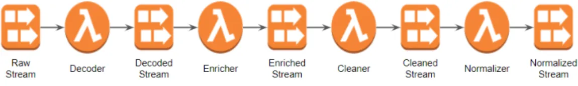
Currently, Scania already has a data pre-processing pipeline working in pro-duction which is shown in Figure 3.1. This pipeline is constructed with Ki-nesis data streams and lambda functions. Messages generated from vehicles sent into pipeline through Kinesis data streams, in the pipeline, data will go through Decoder,Enricher,Cleaner andNormalizer four components, every step connected with each other also with data streams.
Decoder
Decoder is converting messages with various data schema to a fixed internal data schema used in the pipeline. As we mentioned before, Scania has a large number of connected vehicles, different versions of vehicles have dif-ferent sensor systems. For example, old trucks have fewer sensors installed and fewer data collected, however, new generation trucks have up to date controlling system with much more sensor data collected. Hench, the data schema of generated real-time sensor data is varying based on the version of vehicle. Decoder reads messages with vehicle-related schema and produce messages with the unified internal schema. After decoding, other components can process messages with only using one type of data schema.
Enricher
Enricher is enriching external information into currently received messages. When Enricher receives a batch of messages, It looks up if needed informa-tion already stored in the local cache. This local cache mechanism relays on that lambda might reuse function instance. If Enricher cannot find need-to-enrich data in the local cache, it does a batch fetch from DynamoDB tables which are used as an external cache. If there is still missing external data for some messages, it will go to the original API and fetch from there one by one. In the meanwhile, Enricher writes fetched data into DynamoDB to complete the external cache.
Cleaner
Cleaner is cleaning dirty data. The raw data pipeline received from vehi-cles could be no timestamps, out of order, broken messages with error value inside. Cleaner uses predefined cleaning rules to clean errors in received mes-sages. For example, whenCleaner detects duplicated messages and messages without timestamps, it will throw them away as this kind of messages are invaluable. When receiving out of order messages, Cleaner would keep this message and reorder with the next coming message, if the expected unordered message arriving too late,Cleaner will throw them away. Moreover, Cleaner also corrects data inconsistency. From a single vehicle, there exist data fields which suppose to be monotonically increasing. By checking the previous and following value in surrounded messages, Cleaner can detect wrong value or spikes in the stream data items. As lambda is stateless, persistent states required by lambda should be stored in external storage. Cleaner uses Dy-namoDB tables to manage states and a count-based sliding windowing for
data consistency.
Normalizer
Normalizer is normalizing data unit. For example, normalizing all the non-seconds unit to non-seconds, or changing meters to kilometers. Normalizer makes sure all the data fields can have the same unit for further analyzing.
Benchmarking Environment
In order to compare the performance of different solutions. It is necessary to have a standard test environment that can easily change the main com-ponents of different implementations and measure the results, keeping other external components the same. In this chapter, we will introduce a bench-marking test environment designed for our pipeline.
4.1
Motivation
Considering the enormous development of stream processing frameworks, is-suing clear guidelines for choosing an appropriate framework to meet product needs has been becoming challenging. Researchers have invested lots of ef-fort into a comparison of different streaming frameworks with different focus [24] [29]. Study [24] presents a StreamBench with a wide range of operators as metrics to evaluate stream frameworks such as Apache Spark and Storm. The result it concludes is that Spark has higher throughput with fewer node failures. On the other hand, the study [29] presents a setup that allows mea-suring the latency of each separate stage of the pipeline. Yahoo conducts another benchmarking framework [17] for Spark, Storm, and Flink. It uses Apache Kafka for event data transfer and Redis as external storage to mea-sure the performance of example data sets going through some operations such as join, filter, and windowing.
The performance measurement of Scania pipeline is even more compli-cated as there are several unchangeable requirements.
• setup a running pipeline without changing core components
• producing a controllable amount of streaming data to feed current pipeline
• keep the consistency of data schema and using protobuf
• latency measurement for each stage of the pipeline
In existing DEV or TEST environment, there is no high volume of real-time data source. In a production environment where it has a data source, how-ever, first of all, it is difficult to share the same data source without causing issues in the current running product, which might also increase the complex-ity in debugging and tracking product problems. Secondly, data volume in the production environment is stable, in performance testing, one important step is stress testing, which can guide us to design a robust system to handle any occurring peaks. As the number of connected vehicles is becoming more widespread, and thus more data needs to be processed through our pipeline with time pass by. Apart from that, when testing performance, it is necessary to change the configuration of pipeline, for example, the memory of lambda functions, the batch size for each execution, to see how pipeline behaves. These cost effort to manage because of limitations and permissions in the production environment. Considering all these concerns, we design a bench-marking test environment which can produce as much data as we want for stress testing and also have the flexibility of changing configurations without affecting the current product, such as memory resources.
The performance of our pipeline benchmarking focuses on throughput and latency. Throughput can be measured by using Amazon CloudWatch with KDS stream-level metrics with incoming records. Latency is a little complicated as there is no straightforward way of measuring it. It is necessary to design a latency measurement service for this pipeline.
4.2
Benchmarking Design
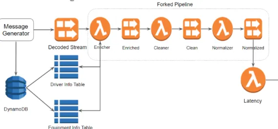
The idea of this Benchmarking test environment is having a component as a data producer, which continuously writes data into our pipeline, and then building a latency measurement service at the end of the pipeline, which can easily measure latency in each component and end-to-end latency. By using this way, the workload, pipeline configuration, and latency monitoring are under the control. The whole architecture can be seen in Figure 4.1.
There are two main components in this Benchmarking environment. One is a message generator. This generator works for:
• Simulating a big amount of trucks with initial values in messages fol-lowing the internal data schema
Figure 4.1: Benchmarking test environment
• Generating needed external enriching information associated with each truck and storing them into DynamoDB tables
• Continuously updating some fields of initial truck messages and writing them to Kinesis data streams
The message generator is a Python program. The number of vehicles and the frequency of updating and sending messages is configurable parameters. With changing values in the configure file, it is easy to make up any work-loads as needed. As we test it local, one thread runs full time without any sleeping delay between updating messages. This generator can push more than 60k messages per minute into Kinesis stream, which is the maximum amount of records Kinesis stream can manage in one minute without losing any data. Compare Figure 3.1 with Figure 4.1, you can see that we use message generator to produce data into decoded KDS, there is no Decoder component in this benchmarking environment. The reason why we remove Decoder is that Decoder here is transforming incoming data with different schema into unified schema used inside of pipeline. The types of data schema depend on the types of system running on vehicles. Our message generator only generates messages with internal schema, which is the result ofDecoder. The other important component is the latency measurement function. When messages go through our pipeline, each component adds message meta-data into them including the timestamp when messages arrive and leave this component. This function attaches in the end of this pipeline. It works for:
• Reading messages from Normalized Kinesis stream and deserializing them
• Extracting message metadata from each received message
• Calculating latency based on message metadata. Such as enricherLatency = enriched timestamp - decoded timestamp
• Creating Customer CloudWatch metrics and pushing the results into them
4.3
Benchmarking Setup
In order to keep the consistency of pipeline behaviours, we set up this bench-marking testing environment with forked pipeline Lambda functions, which are exactly as same as what used in the production environment. We deploy these components in AWS DEV environment with two modifications includ-ing the number of shards and tables required by Enricher. First of all, as current PROD environment is overscale with KDS shards in order to handle unexpected peaks, which cause a problem that lambda functions do not have a full batch of records in executions sometimes. Hence, we reduce all shards configuration to 1 to make sure every execution processes a full batch. In this way, we can have a better view of the relation between throughput and latency. Second, we replace the table names configured in Enricher to table names written in message generator. Ideally, after a cold start, most of the external data elements should be stored in DynamoDB tables locally, only a few of them still need to go external API to fetch. Here we assume that all require external information is already in DynamoDB. This is not a perfect design for the testing environment as it should cause the modification of the original program which needs to be measured, we will discuss a better solu-tion in the next chapter. In the end, the message generator runs locally and continuously producing data to this forked pipeline.
Pipeline Performance
In this chapter, we are going to have an investigation of our current pipeline, in order to understand the performance of pipeline as well as which parts of our pipeline contribute to the latency. The investigation contains several different types of experiments by changing settings such as batch size or memory to see how pipeline behaviors change. In the end, we give some suggestions regarding the best configuration of our current pipeline based on our analyzing results.
5.1
Background
The performance we concern about this pipeline is throughput and latency. There is no experiments of throughput as throughput can be easily detected from CloudWatch and the number of throughput can be scaled with adjusting the number of KDS shards. However, latency is the difficult part to measure. From previous sections we know that when a message comes into our pipeline has to go through KDSs and Lambdas, ideally, the latency of one message should be the accumulation of queuing time in KDS, transmitting time from KDS to Lambda function, and time usage inside of Lambda function. Among all these time usages, the lambda time is the most important value we should measure as it decides how fast this pipeline could be, which also affects the number of messages it can process or throughput in other words. We already know that AWS helps measure lambda running time with Duration metric in CloudWatch. Time consumption in KDS and transferring between components is not as straightforward as lambda execution time which will be measured with our latency function service.
In the following sections, we show how we evaluate duration changes with various combinations of batch sizes and memory which are key aspects
affecting duration, and generally how components latency behaves.
5.2
Experiments
It is important to understand that in our lambda functions, which parts con-tribute to execution time. According to AWS official documentation [10], the given memory of Lambda function influences lambda execution perfor-mance. As the memory size decides the CPU core and network bandwidth this lambda function can use in running time. For example, as AWS says, giving 1792 MB memory is equivalent of assigning 1 full vCPU, and lambda with 512 MB memory allocates approximately twice CPU power compared with lambda with 256 MB memory. Meanwhile, besides memory, batch size contributes a lot to duration, since batch size defines the number of mes-sages lambda needs to process in each round. The bigger batch size we give, the more messages we process per execution, the higher throughput we can achieve. But it is also so obvious that processing 400 records take more time compared with processing 200 items. However, it is difficult to calculate in theory how much execution time we can save with increasing memory or re-duce batch size. Moreover, for a high volume data streaming with a large amount of throughput, if it is worth trading latency with throughput is an-other hard question. In detail, insides of lambda functions, the main tasks are reading and writing from and to DynamoDB, internal processing records from KDS. The speed of communications with DynamoDB is determined by the number of items to send and retrieve which is related to batch size, and network bandwidth which is related to memory allocation. Time usage of internal records processing changes from function to function which depends on weather functions are CPU-intensive or not. Therefore, we assume that both memory and batch size are dedicated to running time and we have done the following experiments to make them clear. For each component, we test
• fixed memory settings with incremental batch size(such as 100, 200, 300, 400)
• fixed batch size with changed memory(such as 512, 640, 1024, 1792) For each configuration, we run thousands of tests. We also enable logging in lambda functions which can tell us the number receiving records in each execution and time consuming for each step including DynamoDB time and main tasks time. An example experiment logging table can be see in Table 5.1.
Memory Size Batch Size process records Duration Read from DB Cleaning Write to DB
1024 MB 200 200 0.968 ms 0.088 ms 0.560 ms 0.137 ms
Table 5.1: Example Experiment Table
5.3
Results Evaluation
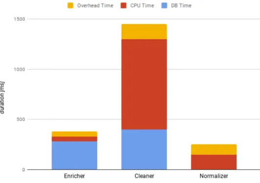
With having thousands of running results as Table 5.1, it is easy to analyze the time-consuming tasks in each pipeline component. First of all, it is better to know, in general, for each component, which task contributes most processing time. As you can see from the Figure 5.1, Enricher duration is mainly contributed by DynamoDB time usage. In contrast, the duration of Cleaner is composed of cleaning time and DynamoDB time and cleaning time is much higher than DB time. Normalizer is a light process which unifies standard units of every parameter, therefore, it has no DB time. The interesting thing in Normalizer is the real records processing time is just around half of the duration.
With understanding core parts result in latency in each component, it is time to show how memory and batch size change the latency. Here we use the results of Cleaner lambda function to demonstrate how memory and batch size dominate execution time. We do not put all test results here, as Enricher and Normalizer have similar behaviours.
Changing Batch Size with Same Memory
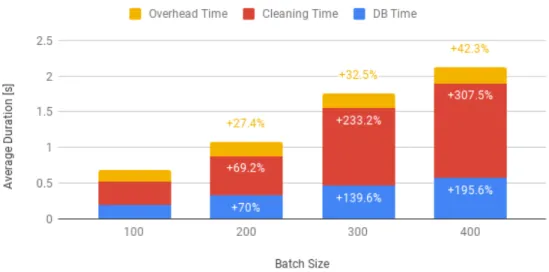
Figure 5.2: Cleaner Duration Breakdown
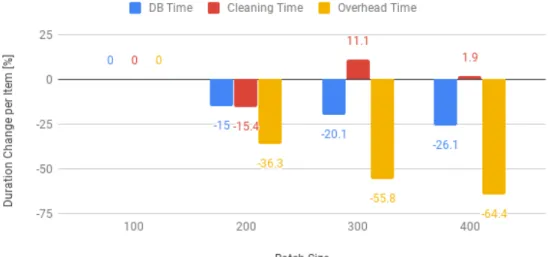
Figure 5.2 illustrates that how batch size affects the Lambda duration when it is under the same memory configuration. The results you can see from Figure 5.2 confirm that a larger batch size increases the overall exe-cution time of the Lambda, but decreases the ratio between running time and a number of items processed. Meanwhile, the overall throughput of the function increases with the number of items in the batch.
It is interesting to know how the execution time changes among different sub-tasks of the Cleaner. To ease this analysis, Figure 5.3 shows the percent-age increase of the per-item execution time, for instance, the execution time divided by the number of items in the batch, for the three sub-tasks of the function.
The cleaning time, which is the time spent processing each item one by one to perform the actual logic of the Cleaner Lambda, increases more or
Figure 5.3: Cleaner Per-Item Duration Comparison
less linearly with the number of items, with the per-item duration fluctuating around the same value for all batch sizes. This is expected, as the same number of calculations needs to be performed sequentially on each item. On the other hand, the time spent reading from and writing to the DynamoDB table, which holds the cleaning windows, grows quite slowly with the number of items. This happens because the reads and writes to the database are not sent one by one, but in batch or groups. Bigger batch sizes can better exploit the capacity of the chunks, and thus incur lower per-item duration. But the execution overhead is the part of the Lambda that shows the greatest decrease in per-item duration as the batch size is increased. This overhead task collects all time spent in the initialization and teardown of the lambda, along with any other time lost outside of the other two tasks. As almost all of this overhead is incurred once per Lambda call, it grows very slowly with the number of items and is thus better amortized by bigger batch sizes.
While the results shown in the figures refer to theCleaner Lambda, sim-ilar patterns have emerged from all functions: processing time grows linearly with the number of items, database access time grows quite slowly, thanks to batching, while overheads show only a tiny increase. Thus, overall, increasing batch sizes is a useful optimization for functions whose duration is dominated by database accesses, or for functions that are so quick that overhead times represent a significant portion of their execution.
According to these results, increasing the batch size of theCleanerLambda would only achieve marginal throughput increases, as its execution time is dominated by actual computations. On the other hand, the Enricher func-tion would benefit from a large number of items, as it spends most of its time performing database reads. The Normalizer Lambda does not access any database, but processes items so quickly that an increase in batch size might have a visible positive effect, by greatly reducing the function call overhead.
Changing Memory Size with Same Batch Size
Figure 5.4: Cleaner Memory Analysis
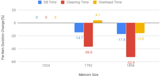
From the results in Figure 5.4, it can be seen that, as expected, a higher memory allocation has a positive effect on the overall runtime of the Cleaner Lambda, thanks to the higher CPU power available. One small fluctuation aside, all activities within the function benefit from more computational re-sources, but they show very different speedups, as highlighted in Figure 5.5. The cleaning time, being a computationally-intensive task, shows the greatest speedups, as more CPU power directly translates to more items processed per unit of time. The database access also speeds up, but by a much smaller margin, as it can be assumed that most of the time is spent waiting, due to network latencies and due to the processing time required
Figure 5.5: Cleaner Per-Item Duration Comparison with Different Memory by the DynamoDB server. It is interesting to note that the overhead time does not seem to be affected so much by the increase in CPU power. This goes against the assumption that more computational power would provide better startup times. A possible explanation might be that these overheads are not entirely managed by the Lambda container itself, but by some other component in the Lambda server, which does not scale with the container resources.
As for the analysis of batch sizes, the results obtained for the Enricher andNormalizer mirror the ones for theCleaner, that was reported here. The findings support the idea that the memory size should be increased for those functions whose execution is dominated by CPU-intensive processing tasks. On the other hand, it should be kept low for network-intensive or lightweight functions, in order to reduce costs.
To summarize these findings, in our pipeline, Cleaner is CPU-bound, increasing the memory of cleaning Lambda can speed up execution time and also increase throughput. Enricher is IO-bound, increasing memory has little help with Enricher, however, increasing batch size to better utilize the batch read capabilities of DynamoDB. Normalizer is a light function which has no strict actions needed. It is better to keep it as now or increase the batch size to reduce overheads and optimize costs.
5.4
Latency Discussion
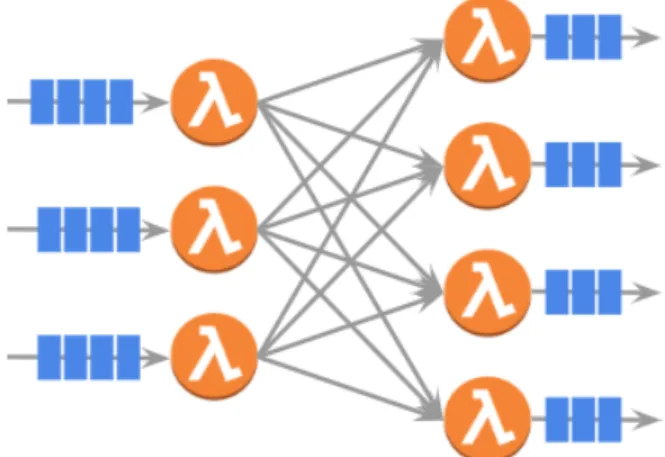
Apart from Lambda duration, there is another significant effect contributing to pipeline latency. That is the relationship between KDS shard and Lambda batch size. Our pipeline uses Kinesis Data Streams and Lambda functions. From AWS official documents [11], it says that lambda polls each KDS shard at a base rate of once per second. If more records in KDS are available, Lambda keeps processing batches until it receives a batch that is smaller than the configured batch size. It means if we oversize the batch size, it will cause one second polling delay as the incoming records cannot keep feeding the lambda as it needs. In the current Scania pipeline, it has three Lambdas connected with KDS. The best setting of KDS shard and Lambda batch size should be like Figure 5.6.
Figure 5.6: Best Settings of KDS Shard and Lambda Batch Size As it is shown in Figure 5.6, data goes through two Lambda functions, here we can call them as upstream lambda and downstream lambda. The best configuration is, for example, if we have 3 KDS shards(each shard has one corresponding Lambda function) and Lambda batch size is 4 in upstream, then when the downstream has 4 KDS shards / Lambda functions, we should let the Lambda batch size change to 3. The equation can be:
downstream Lambda batch size * downstream KDS shards = upstream Lambda batch size * upstream KDS shards - dropped error messages
Alternative Solution
There are several stream processing frameworks appearing in the past few years aiming for different purposes and a variety of use cases. Such as STREAM and Aurora coming out of university labs in earlier ages, open-source frameworks from Apache foundation and services build by cloud providers. These streaming frameworks internally implemented with its own advanced technologies to manage increased challenges in stream processing. However, it is hard to say, in general, which framework outperforms the others as each of them can become the desirable choice in certain circumstances with designed constraints.
Several existing studies have already provided comparative results of com-mon frameworks with chosen metrics such as latency, throughput and re-source usages. For example, study [23] compares the performance of three main streaming frameworks including Storm, Spark and Flink with Yahoo Streaming Benchmark (YSB). These frameworks are evaluated with satura-tion level which is the maximum streaming workload they can handle with-out creating extra delay. The study concludes that with saturation levels of event processing per second, Flink has the best performance compared with the other two, it is able to process much more events with less resource usage (worker nodes). Spark is able to outperform the left by increasing batching interval to achieve highest throughput per second, however, it also means the latency compromise. Another thesis study [30] uses a tool to bench-mark performance of Spark Streaming, Flink and Storm. This tool produces workloads designed to evaluate performance of frameworks with processing basic operators as well as Join and Iterator operators. The study shows that Spark Streaming and Flink achieves significantly higher throughput than Storm. however, because of micro-batch computation, Spark Streaming has a trade-off between latency and throughput. Therefore, as the author said, in practice, Flink can achieve both low latency and high throughput in most
stream processing cases.
Our stream processing system uses AWS Lambda functions. As we talked before, these components of our system have some special requirements. For example, the input data format is protocol buffers, the Enricher component has to enrich streaming data with external dynamic data. Therefore, apart from latency and throughput, we should also take into consideration such as data format, fetch external data when we compare these frameworks.
In the following sections, we will first introduce some data streaming systems we selected, and give a comparison with selected features.
6.1
Overview of Streaming Frameworks
Apache Spark streaming is an extension of Spark which is designed for build-ing scalable fault-tolerant streambuild-ing applications. Spark streambuild-ing system divides incoming data streams into micro-batches and stores them in mem-ory. It takes each batch of input data as Resilient Distributed Datasets (RDDs) and processes these batches by using scheduled spark job with RDD operations. It also output processed results as streams of batches and push them into database or file systems [4].
Apache Flink is a distributed processing engine for stateful computatio
![Figure 2.1: Overview of CRISP and tasks[31]](https://thumb-us.123doks.com/thumbv2/123dok_us/61511.2507236/13.892.154.740.255.478/figure-overview-of-crisp-and-tasks.webp)
![Figure 2.2: A Simple Dataflow Model (Source: [16])](https://thumb-us.123doks.com/thumbv2/123dok_us/61511.2507236/17.892.194.707.784.979/figure-a-simple-dataflow-model-source.webp)