Languages, and Digital Logic

Chapter 2

: Machines, Machine

Languages, and Digital Logic

Topics

2.1 Classification of Computers and Their Instructions 2.2 Computer Instruction Sets

2.3 Informal Description of the Simple RISC Computer, SRC

2.4 Formal Description of SRC Using Register Transfer Notation, RTN

2.5 Describing Addressing Modes with RTN

2.6 Register Transfers and Logic Circuits: From Behavior to Hardware

What Are the Components of an ISA?

• Sometimes known as The Programmer’s Model of the machine

• Storage cells

• General and special purpose registers in the CPU

• Many general purpose cells of same size in memory

• Storage associated with I/O devices

• The machine instruction set

• The instruction set is the entire repertoire of machine operations

• Makes use of storage cells, formats, and results of the fetch/ execute cycle

• i.e., register transfers

• The instruction format

• Size and meaning of fields within the instruction

• The nature of the fetch-execute cycle

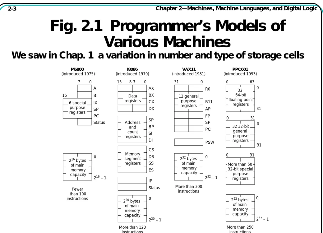
Fig. 2.1 Programmer’s Models of

Various Machines

We saw in Chap. 1 a variation in number and type of storage cells

216 bytes of main memory capacity Fewer than 100 instructions 7 15 A 216 – 1 B IX SP PC 0 12 general purpose registers More than 300 instructions More than 250 instructions More than 120 instructions 232 – 1 252 – 1 0 PSW Status R0 PC R11 AP FP SP 0 31 0 32 64-bit floating point registers (introduced 1993) (introduced 1981) (introduced 1975) (introduced 1979) 0 31 0 63 32 32-bit general purpose registers 0 31 0 31 More than 50 32-bit special purpose registers 0 31 252 _bytes of main memory capacity 0 M6800 VAX11 PPC601 220 – 1 AX BX CX DX SP BP SI DI 15 87 0 IP Status Address and count registers CS DS SS ES Memory segment registers 220 _bytes of main memory capacity 0 I8086 232 bytes of main memory capacity Data registers 6 special purpose registers

• Which operation to perform add r0, r1, r3

• Ans: Op code: add, load, branch, etc.

• Where to find the operand or operands add r0, r1, r3

• In CPU registers, memory cells, I/O locations, or part of instruction

• Place to store result add r0, r1, r3

• Again CPU register or memory cell

• Location of next instruction add r0, r1, r3

br endloop

• Almost always memory cell pointed to by program counter—PC

• Sometimes there is no operand, or no result, or no next instruction.

Can you think of examples?

What Must an Instruction Specify?

Instructions Can Be Divided into

3 Classes

• Data movement instructions

• Move data from a memory location or register to another memory location or register without changing its form

• Load—source is memory and destination is register

• Store—source is register and destination is memory

• Arithmetic and logic (ALU) instructions

• Change the form of one or more operands to produce a result stored in another location

• Add, Sub, Shift, etc.

• Branch instructions (control flow instructions)

• Alter the normal flow of control from executing the next instruction in sequence

Tbl 2.1 Examples of Data Movement

Instructions

• Lots of variation, even with one instruction type

Instruction Meaning Machine

MOV A, B Move 16 bits from memory location A to VAX11

Location B

LDA A, Addr Load accumulator A with the byte at memory M6800

location Addr

lwz R3, A Move 32-bit data from memory location A to PPC601

register R3

li $3, 455 Load the 32-bit integer 455 into register $3 MIPS R3000

mov R4, dout Move 16-bit data from R4 to output port dout DEC PDP11

IN, AL, KBD Load a byte from in port KBD to accumulator Intel Pentium

Tbl 2.2 Examples of ALU

Instructions

Instruction Meaning Machine

MULF A, B, C multiply the 32-bit floating point values at VAX11 mem loc’ns. A and B, store at C

nabs r3, r1 Store abs value of r1 in r3 PPC601

ori $2, $1, 255 Store logical OR of reg $ 1 with 255 into reg $2 MIPS R3000

DEC R2 Decrement the 16-bit value stored in reg R2 DEC PDP11

SHL AX, 4 Shift the 16-bit value in reg AX left by 4 bit pos’ns. Intel 8086

Tbl 2.3 Examples of Branch

Instructions

Instruction Meaning Machine

BLSS A, Tgt Branch to address Tgt if the least significant VAX11 bit of mem loc’n. A is set (i.e. = 1)

bun r2 Branch to location in R2 if result of previous PPC601 floating point computation was Not a Number (NAN)

beq $2, $1, 32 Branch to location (PC + 4 + 32) if contents MIPS R3000 of $1 and $2 are equal

SOB R4, Loop Decrement R4 and branch to Loop if R4 ≠ 0 DEC PDP11

CPU Registers Associated with Flow of

Control—Branch Instructions

• Program counter usually locates next instruction

• Condition codes may control branch

• Branch targets may be separate registers

Processor State C N V Z Program Counter Branch Targets Condition Codes • • •

HLL Conditionals Implemented by

Control Flow Change

• Conditions are computed by arithmetic instructions

• Program counter is changed to execute only instructions associated with true conditions

C language

Assembly language

if NUM==5 then SET=7

CMP.W #5, NUM

BNE L1

MOV.W #7, SET

L1 ...

CPU Registers May Have a

“Personality”

• Architecture classes are often based on how where the

operands and result are located and how they are specified by the instruction.

• They can be in CPU registers or main memory:

Top Second

Stack Arithmetic

Registers AddressRegisters General Purpose_Registers Push Pop • • • • • • • • • • • •

Stack Machine Accumulat or Machine General Regist er Machine

3-, 2-, 1-, & 0-Address ISAs

• The classification is based on arithmetic instructions that have two operands and one result

• The key issue is “how many of these are specified by memory addresses, as opposed to being specified implicitly”

• A 3-address instruction specifies memory addresses for both operands and the result R ← Op1 op Op2

• A 2-address instruction overwrites one operand in memory with the result Op2 ← Op1 op Op2

• A 1-address instruction has a processor, called the accumulator register, to hold one operand & the result (no addr. needed)

Acc ← Acc op Op1

• A 0-address + uses a CPU register stack to hold both operands and the result TOS ← TOS op SOS (where TOS is Top Of Stack, SOS is Second On Stack)

• The 4-address instruction, hardly ever seen, also allows the address of the next instruction to specified explicitly

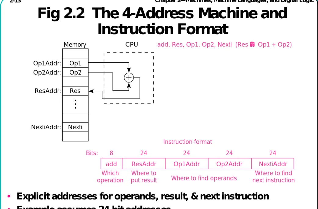
Fig 2.2 The 4-Address Machine and

Instruction Format

• Explicit addresses for operands, result, & next instruction

• Example assumes 24-bit addresses

• Discuss: size of instruction in bytes

Memory Op1Addr: Op2Addr: Op1 Op2 ResAddr: NextiAddr: Bits: 8 24 24 Instruction format 24 24 Res Nexti

CPU add, Res, Op1, Op2, Nexti (Res ← Op1 + Op2)

add ResAddr Op1Addr Op2Addr NextiAddr

Which operation

Where to

put result Where to find operands

Where to find next instruction

Instruction Format

• Address of next instruction kept in processor state register— the PC (except for explicit branches/jumps)

• Rest of addresses in instruction

Memory Op1Addr: Op2Addr: Op1 Program counter Op2 ResAddr: NextiAddr: Bits: 8 24 24 Instruction format 24 Res Nexti CPU Where to find next instruction 24

add, Res, Op1, Op2 (Res ← Op2 + Op1)

add ResAddr Op1Addr Op2Addr

Which operation

Where to

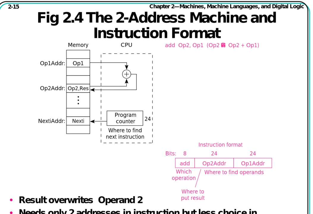
Fig 2.4 The 2-Address Machine and

Instruction Format

• Result overwrites Operand 2

• Needs only 2 addresses in instruction but less choice in placing data Memory Op1Addr: Op2Addr: Op1 Program counter Op2,Res Nexti NextiAddr: Bits: 8 24 24 Instruction format CPU Where to find next instruction 24

add Op2, Op1 (Op2 ← Op2 + Op1)

add Op2Addr Op1Addr Which

operation Where to put result

Instruction Format

• Special CPU register, the accumulator, supplies 1 operand and stores result

Need instructions to load and store operands:

LDA OpAddr STA OpAddr

Memory

Op1Addr: Op1

Nexti Program_counter Accumulator NextiAddr: Bits: 8 24 Instruction format CPU Where to find next instruction 24

add Op1 (Acc ← Acc + Op1)

add Op1Addr Which operation Where to find operand1 Where to find operand2, and where to put result

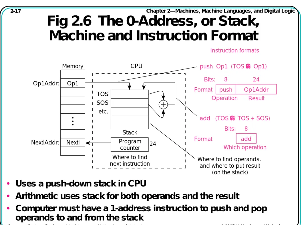
Fig 2.6 The 0-Address, or Stack,

Machine and Instruction Format

• Uses a push-down stack in CPU

• Arithmetic uses stack for both operands and the result

• Computer must have a 1-address instruction to push and pop operands to and from the stack

Memory Op1Addr: TOS SOS etc. Op1 Program counter NextiAddr: Nexti Bits: Format Format 8 24 CPU Where to find next instruction Stack 24

push Op1 (TOS ← Op1) Instruction formats

add (TOS ← TOS + SOS) push Op1Addr Operation Bits: 8 add Which operation Result

Where to find operands, and where to put result

Example 2.1 Expression Evaluation for

3-, 2-, 1-, and 0-Address Machines

• Number of instructions & number of addresses both vary

• Discuss as examples: size of code in each case

3 - a d d r e s s

2 - a d d r e s s

1 - a d d r e s s

S t a c k

add a, b, c

mpy a, a, d

sub a, a, e

load a, b

add a, c

mpy a, d

sub a, e

load b

add c

mpy d

sub e

store a

push b

push c

add

push d

mpy

push e

sub

pop a

Evaluat e a = (b+c)*d - e

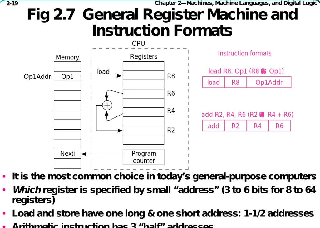
Fig 2.7 General Register Machine and

Instruction Formats

• It is the most common choice in today’s general-purpose computers

• Which register is specified by small “address” (3 to 6 bits for 8 to 64

registers)

• Load and store have one long & one short address: 1-1/2 addresses

• Arithmetic instruction has 3 “half” addresses

Memory

Op1Addr: Op1 load

Nexti Program

counter

load R8, Op1 (R8 ← Op1)

CPU Registers R8 R6 R4 R2 Instruction formats R8 load Op1Addr add R2, R4, R6 (R2 ← R4 + R6) R2 add R4 R6

Real Machines Are Not So Simple

• Most real machines have a mixture of 3, 2, 1, 0, and 1-1/2 address instructions

• A distinction can be made on whether arithmetic instructions use data from memory

• If ALU instructions only use registers for operands and result, machine type is load-store

• Only load and store instructions reference memory

• Other machines have a mix of register-memory and memory-memory instructions

Addressing Modes

• An addressing mode is hardware support for a useful way of determining a memory address

• Different addressing modes solve different HLL problems

• Some addresses may be known at compile time, e.g., global variables

• Others may not be known until run time, e.g., pointers

• Addresses may have to be computed. Examples include:

• Record (struct) components:

• variable base (full address) + constant (small)

• Array components:

• constant base (full address) + index variable (small)

• Possible to store constant values w/o using another memory cell by storing them with or adjacent to the instruction itself

HLL Examples of Structured Addresses

• C language: rec → count

• rec is a pointer to a record: full address variable

• count is a field name: fixed byte offset, say 24

• C language: v[i]

• v is fixed base address of array: full address constant

• i is name of variable index: no larger than array size

• Variables must be contained in registers or memory cells

• Small constants can be contained in the instruction

• Result: need for “address arithmetic.”

• E.g., Address of Rec → Count is address of Rec + offset of count.

Rec →

Count

V →

Fig 2.8 Common Addressing Modes

(Instruction contains the operand.)

Addr of A Operand Memory Op'n Instr b) Direct Addressing (Instruction contains address of operand) LOAD A, ... Address of address of A Operand Addr Memory Op'n Instr c) Indirect Addressing (Instruction contains address of address of operand) LOAD (A), ... Operand Operand Memory Op'n Instr

d) Register Indirect Addressing

(register contains address of operand)

LOAD [R2], ... R2 . . . R2 Operand Addr. Operand Memory Op'n Instr

e) Displacement (Based) (Indexed) Addressing

(address of operand = register +constant)

LOAD 4[R2], ... R2 4 Operand Addr. + R2 PC Operand Memory Op'n f) Relative Addressing

(Address of operand = PC+constant)

LOADRel 4[PC], ... 4

Operand Addr. +

Example: Computer, SRC

Simple RISC Computer

• 32 general purpose registers of 32 bits

• 32-bit program counter, PC, and instruction register, IR

• 232 bytes of memory address space

R0

R31 PC IR

The SRC CPU Main memory

31 0 7 0 0 R[7] means contents of register 7 M[32] means contents of memory location 32 232 – 1 32 32-bit general purpose registers 232 bytes of main memory

SRC Characteristics

• Load-store design: only way to access memory is through load and store instructions

• Only a few addressing modes are supported

• ALU instructions are 3-register type

• Branch instructions can branch unconditionally or

conditionally on whether the value in a specified register is = 0, <> 0, >= 0, or < 0

• Branch and link instructions are similar, but leave the value of current PC in any register, useful for subroutine return

SRC Basic Instruction Formats

• There are three basic instruction format types

• The number of register specifier fields and length of the constant field vary

• Other formats result from unused fields or parts

• Details of formats on next slide

31 27 26 22 21 0 31 27 27 26 26 22 22 21 21 31 17 16 17 16 12 11 0 0 op r a r b r c r b r a r a op op c1 c2 c3 Type 1 Type 2 Type 3

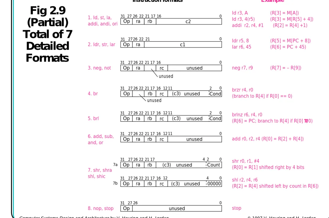
Fig 2.9

(Partial)

Total of 7

Detailed

Formats

addi, andi, ori rb c2

Instruction formats Example

31 27 26 22 21 17 16 0 Id r3, A Id r3, 4(r5) addi r2, r4, #1 (R[3] = M[A]) (R[3] = M[R[5] + 4]) (R[2] = R[4] +1) ra Op 2. Idr, str, lar c1 31 2726 22 21 0 _{Idr r5, 8} Iar r6, 45 (R[5] = M[PC + 8]) (R[6] = PC + 45) ra Op

3. neg, not unused

31 27 26 22 21 17 16 0 neg r7, r9 (R[7] = – R[9]) ra unused rc Op 4. br unused 31 27 26 22 21 1716 1211 2 0 _{brzr r4, r0} (branch to R[4] if R[0] == 0) rb rc (c3) Cond Op 5. brl unused 31 27 26 22 21 17 16 0 _{brlnz r6, r4, r0} (R[6] = PC; branch to R[4] if R[0] ≠ 0) ra rb rc 12 11 2 Cond (c3) Op unused 31 27 26 22 21 17 16 0 _{shl r2, r4, r6}

(R[2] = R[4] shifted left by count in R[6])

ra rb rc 12 4 4 00000 (c3) Op 7. shr, shra shl, shic unused 31 27 26 22 7a 7b 21 17 0 _{shr r0, r1, #4}

(R[0] = R[1] shifted right by 4 bits

ra rb 2 Count Op 6. add, sub, and, or unused 31 27 26 22 21 17 16 0 add r0, r2, r4 (R[0] = R[2] + R[4]) ra rb rc 12 11 Op

8. nop, stop unused

31 27 0 stop 26 unused (c3) (c3) (c3)

Tbl 2.4 Example SRC Load and Store

Instructions

• Address can be constant, constant + register, or constant + PC

• Memory contents or address itself can be loaded

(note use of la to load a constant)

Instruction op ra rb c1 Meaning Addressing Mode ld r1, 32 1 1 0 32 _R[1] ← _M[32] Direct ld r22, 24(r4) 1 22 4 24 _R[22] ← _M[24+R[4]] Displacement st r4, 0(r9) 3 4 9 0 _M[R[9]] ← _R[4] Register indirect la r7, 32 5 7 0 32 _R[7] ← ₃₂ Immediate ldr r12, -48 2 12 – -48 _R[12] ← _{M[PC -48]} Relative lar r3, 0 6 3 – 0 _R[3] ← _PC Register (!)

Assembly Language Forms of

Arithmetic and Logic Instructions

• Immediate subtract not needed since constant in addi may be negative

Format Example Meaning

neg ra, rc neg r1, r2 ;Negate (r1 = -r2) not ra, rc not r2, r3 ;Not (r2 = r3´ )

add ra, rb, rc add r2, r3, r4 ;2’s complement addition

sub ra, rb, rc ;2’s complement subtraction

and ra, rb, rc ;Logical and

or ra, rb, rc ;Logical or

addi ra, rb, c2 addi r1, r3, #1 ;Immediate 2’s complement add

andi ra, rb, c2 ;Immediate logical and

Branch Instruction Format

There are actually only two branch instructions:

br rb, rc, c3<2..0> ; branch to R[rb] if R[rc] meets ; the condition defined by c3<2..0>

brl ra, rb, rc, c3<2..0> ; R[ra] ← PC; branch as above

lsbs condition Assy language form Example

000 never brlnv brlnv r6 001 always br, brl br r5, brl r5 010 if rc = 0 brzr, brlzr brzr r2, r4, r5 011 if rc ≠ 0 brnz, brlnz 100 if rc ≥ 0 brpl, brlpl 101 if rc < 0 brmi, brlmi

• It is c3<2..0>, the 3 lsbs of c3, that governs what the branch condition is:

• Note that branch target address is always in register R[rb].

Tbl 2.6 Forms and Formats of the

br

and

brl

Instructions

Ass’y lang.

Example instr. Meaning op ra rb rc c3

〈2..0〉 Branch Cond’n. brlnv brlnv r6 _R[6] ← _PC 9 6 — — 000 never br br r4 _PC ← _R[4] 8 — 4 — 001 always brl brl r6,r4 _R[6] ← _PC; PC ← R[4] 9 6 4 — 001 always brzr brzr r5,r1 if (R[1]=0) PC ← R[5] 8 — 5 1 010 zero brlzr brlzr r7,r5,r1 _R[7] ← _PC; 9 7 5 1 010 zero brnz brnz r1, r0 _{if (R[0]}≠_{0) PC}← _{R[1] 8} — 1 0 011 nonzero brlnz brlnz r2,r1,r0 _R[2] ← _PC; if (R[0]≠0) PC← R[1] 9 2 1 0 011 nonzero brpl brpl r3, r2 _{if (R[2]}≥_{0) PC}← _{R[3] 8} — 3 2 100 plus brlpl brlpl r4,r3,r2 _R[4] ← _PC; if (R[2]≥0) PC← R[3] 9 4 3 2 plus

brmi brmi r0, r1 _{if (R[1]<0) PC}← _{R[0] 8} — 0 1 101 minus

brlmi brlmi r3,r0,r1 _R[3] ← _PC;

if (r1<0) PC← R[0]

Branch Instructions—Example

C: goto Label3 SRC:

lar r0, Label3 ; put branch target address into tgt reg.

br r0 ; and branch

• • •

Example of Conditional Branch

in C: #define Cost 125 if (X<0) then X = -X; in SRC:

Cost .equ 125 ;define symbolic constant

.org 1000 ;next word will be loaded at address 1000₁₀

X: .dw 1 ;reserve 1 word for variable X

.org 5000 ;program will be loaded at location 5000₁₀

lar r0, Over ;load address of “false” jump location ld r1, X ;load value of X into r1

brpl r0, r1 ;branch to Else if r1≥0 neg r1, r1 ;negate value

RTN (Register Transfer Notation)

• Provides a formal means of describing machine structure and function

• Is at the “just right” level for machine descriptions

• Does not replace hardware description languages

• Can be used to describe what a machine does (an

abstract RTN) without describing how the machine

does it

• Can also be used to describe a particular hardware implementation (a concrete RTN)

RTN (cont’d.)

• At first you may find this “meta description” confusing, because it is a language that is used to describe a

language

• You will find that developing a familiarity with RTN will aid greatly in your understanding of new machine

design concepts

Some RTN Features—

Using RTN to Describe a Machine’s

Static Properties

Static Properties

• Specifying registers

• IR〈31..0〉 specifies a register named “IR” having 32 bits numbered 31 to 0

• “Naming” using the := naming operator:

• op〈4..0〉 := IR〈31..27〉 specifies that the 5 msbs of IR be called op, with bits 4..0

• Notice that this does not create a new register, it just

generates another name, or “alias,” for an already existing register or part of a register

Using RTN to Describe

Dynamic Properties

Dynamic Properties

• Conditional expressions:

(op=12) → R[ra] ← R[rb] + R[rc]: ; defines the add instruction

“if” condition “then” RTN Assignment Operator

This fragment of RTN describes the SRC add instruction. It says, “when the op field of IR = 12, then store in the register specified by the ra field, the result of adding the register specified by the rb field to the register specified by the rc field.”

Using RTN to Describe the SRC (Static)

Processor State

Processor state

PC

〈

31..0

〉

: program

counter

(memory addr. of next inst.)

IR

〈

31..0

〉

:

instruction register

Run:

one bit run/halt indicator

Strt:

start signal

RTN Register Declarations

• General register specifications shows some features of the notation

• Describes a set of 32 32-bit registers with names R[0] to R[31]

R[0..31]

〈

31..0

〉

:

Memory Declaration:

RTN Naming Operator

• Defining names with formal parameters is a powerful formatting tool

• Used here to define word memory (big-endian)

Main memory state

Mem[0..2

_{- 1]}

〈

_7..0

〉

_:

₂

_{addressable bytes of memory}

M[x]

〈

31..0

〉

:= Mem[x]#Mem[x+1]#Mem[x+2]#Mem[x+3]:

RTN Instruction Formatting Uses

Renaming of IR Bits

Instruction formats

op

〈

4..0

〉

:= IR

〈

31..27

〉

: operation code field

ra

〈

4..0

〉

:= IR

〈

26..22

〉

:

target register field

rb

〈

4..0

〉

:= IR

〈

21..17

〉

:

operand, address index, or

branch target register

rc

〈

4..0

〉

:= IR

〈

16..12

〉

:

second operand, conditional

test, or shift count register

c1

〈

21..0

〉

:= IR

〈

21..0

〉

: long displacement field

c2

〈

16..0

〉

:= IR

〈

16..0

〉

: short displacement or

immediate field

c3

〈

11..0

〉

:= IR

〈

11..0

〉

: count or modifier field

Specifying Dynamic Properties of SRC:

RTN Gives Specifics of Address

Calculation

• Renaming defines displacement and relative addresses

• New RTN notation is used

• condition → expression means if condition then expression

• modifiers in { } describe type of arithmetic or how short numbers are extended to longer ones

• arithmetic operators (+ - * / etc.) can be used in expressions Register R[0] cannot be added to a displacement

Effective address calculations (occur at runtime):

disp〈31..0〉 := ((rb=0) → c2〈16..0〉 {sign extend}: displacement (rb≠0) → R[rb] + c2〈16..0〉 {sign extend, 2’s comp.} ): address rel〈31..0〉 := PC〈31..0〉 + c1〈21..0〉 {sign extend, 2’s comp.}: relative

Detailed Questions Answered by the

RTN for Addresses

• What set of memory cells can be addressed by direct addressing (displacement with rb=0)

• If c2〈16〉=0 (positive displacement) absolute

addresses range from 00000000H to 0000FFFFH

• If c2〈16〉=1 (negative displacement) absolute

addresses range from FFFF0000H to FFFFFFFFH

• What range of memory addresses can be specified by a relative address

• The largest positive value of C1〈21..0〉 is 221-1 and

its most negative value is -221, so addresses up to

221_{-1 forward and 221 backward from the current PC}

value can be specified

Instruction Interpretation: RTN

Description of Fetch-Execute

• Need to describe actions (not just declarations)

• Some new notation

instruction_interpretation := (

¬

Run

∧

Strt

→

Run

←

1:

Run

→

(IR

←

M[PC]: PC

←

PC + 4; instruction_execution) );

Logical NOT

Logical AND

Register transfer Separates statements

RTN Sequence and Clocking

• In general, RTN statements separated by : take place during the same clock pulse

• Statements separated by ; take place on successive clock pulses

• This is not entirely accurate since some things written with one RTN statement can take several clocks to

perform

• More precise difference between : and ;

• The order of execution of statements separated by : does not matter

• If statements are separated by ; the one on the left must be complete before the one on the right starts

More About Instruction Interpretation

RTN

• In the expression IR ← M[PC]: PC ← PC + 4; which value of PC applies to M[PC] ?

• The rule in RTN is that all right hand sides of “:” -

separated RTs are evaluated before any LHS is changed

• In logic design, this corresponds to “master-slave” operation of flip-flops

• We see what happens when Run is true and when Run is false but Strt is true. What about the case of Run and Strt both false?

• Since no action is specified for this case, the RTN implicitly says that no action occurs in this case

Individual Instructions

• instruction_interpretation contained a forward reference to instruction_execution

• instruction_execution is a long list of conditional operations

• The condition is that the op code specifies a given instruction

• The operation describes what that instruction does

• Note that the operations of the instruction are done after (;) the instruction is put into IR and the PC has been advanced to the next instruction

RTN Instruction Execution for Load and

Store Instructions

• The in-line definition (:= op=1) saves writing a separate definition ld := op=1 for the ld mnemonic

• The previous definitions of disp and rel are needed to understand all the details

instruction_execution := (

ld (:= op= 1) → R[ra] ← M[disp]: load register

ldr (:= op= 2) → R[ra] ← M[rel]: load register relative st (:= op= 3) → M[disp] ← R[ra]: store register

str (:= op= 4) → M[rel] ← R[ra]: store register relative

la (:= op= 5 ) → R[ra] ← disp: load displacement address lar (:= op= 6) → R[ra] ← rel: load relative address

SRC RTN—The Main Loop

ii := instruction_interpretation:

ie := instruction_execution :

ld (:= op= 1) → R[ra] ← M[disp]: Big switch ldr (:= op= 2) → R[ra] ← M[rel]: statement

. . . on the opcode

stop (:= op= 31) → Run ← 0: ); ii

Use of RTN Definitions:

Text Substitution Semantics

• An example:

• If IR = 00001 00101 00011 00000000000001011

• then ld → R[5] ← M[ R[3] + 11 ]: ld (:= op= 1) → R[ra] ← M[disp]:

disp〈31..0〉 := ((rb=0) → c2〈16..0〉 {sign extend}:

(rb≠0) → R[rb] + c2〈16..0〉 {sign extend, 2’s comp.} ):

ld (:= op= 1) → R[ra] ← M[

((rb=0) → c2〈16..0〉 {sign extend}:

(rb≠0) → R[rb] + c2〈16..0〉 {sign extend, 2’s comp.} ): ]:

RTN Descriptions of SRC Branch

Instructions

• Branch condition determined by 3 lsbs of instruction

• Link register (R[ra]) set to point to next instruction cond := ( c3〈2..0〉=0 → 0: never c3〈2..0〉=1 → 1: always c3〈2..0〉=2 → R[rc]=0: if register is zero c3〈2..0〉=3 → R[rc]≠0: if register is nonzero c3〈2..0〉=4 → R[rc]〈31〉=0: if positive or zero c3〈2..0〉=5 → R[rc]〈31〉=1 ): if negative

br (:= op= 8) → (cond → PC ← R[rb]): conditional branch brl (:= op= 9) → (R[ra] ← PC:

RTN for Arithmetic and Logic

• Logical operators: and ∧ or ∨ and not ¬

add (:= op=12)

→

R[ra]

←

R[rb] + R[rc]:

addi (:= op=13)

→

R[ra]

←

R[rb] + c2

〈

16..0

〉

{2's comp. sign

ext.}:

sub (:= op=14)

→

R[ra]

←

R[rb] - R[rc]:

neg (:= op=15)

→

R[ra]

←

-R[rc]:

and (:= op=20)

→

R[ra]

←

R[rb]

∧

R[rc]:

andi (:= op=21)

→

R[ra]

←

R[rb]

∧

c2

〈

16..0

〉

{sign extend}:

or (:= op=22)

→

R[ra]

←

R[rb]

∨

R[rc]:

ori (:= op=23)

→

R[ra]

←

R[rb]

∨

c2

〈

16..0

〉

{sign extend}:

not (:= op=24)

→

R[ra]

←

¬

R[rc]:

RTN for Shift Instructions

• Count may be 5 lsbs of a register or the instruction

• Notation: @ - replication, # - concatenation

n := ( (c3〈4..0〉=0) → R[rc]〈4..0〉: (c3〈4..0〉≠0) → c3〈4..0〉 ):

shr (:= op=26) → R[ra]〈31..0〉← (n @ 0) # R[rb]〈31..n〉:

shra (:= op=27) → R[ra]〈31..0〉← (n @ R[rb]〈31〉) # R[rb]〈31..n〉: shl (:= op=28) → R[ra]〈31..0〉← R[rb]〈31-n..0〉 # (n @ 0):

Example of Replication and

Concatenation in Shift

• Arithmetic shift right by 13 concatenates 13 copies of the sign bit with the upper 19 bits of the operand

shra r1, r2, 13

13@R[2]

〈

31

〉

R[2]

〈

31..13

〉

R[2]=

#

R[1]=

Assembly Language for Shift

• Form of assembly language instruction tells whether to set c3=0

shr ra, rb, rc ;Shift rb right into ra by 5 lsbs of rc shr ra, rb, count ;Shift rb right into ra by 5 lsbs of inst shra ra, rb, rc ;AShift rb right into ra by 5 lsbs of rc shra ra, rb, count ;AShift rb right into ra by 5 lsbs of inst shl ra, rb, rc ;Shift rb left into ra by 5 lsbs of rc

shl ra, rb, count ;Shift rb left into ra by 5 lsbs of inst shc ra, rb, rc ;Shift rb circ. into ra by 5 lsbs of rc shc ra, rb, count ;Shift rb circ. into ra by 5 lsbs of inst

End of RTN Definition of

instruction_execution

• We will find special use for nop in pipelining

• The machine waits for Strt after executing stop

• The long conditional statement defining

instruction_execution ends with a direction to go repeat instruction_interpretation, which will fetch and execute the next instruction (if Run still =1)

nop (:= op= 0) → : No operation

stop (:= op= 31) → Run ← 0: Stop instruction

); End of instruction_execution

Confused about RTN and SRC?

• SRC is a Machine Language

• It can be interpreted by either hardware or software simulator.

• RTN is a Specification Language

• Specification languages are languages that are used to specify other languages or systems—a

metalanguage.

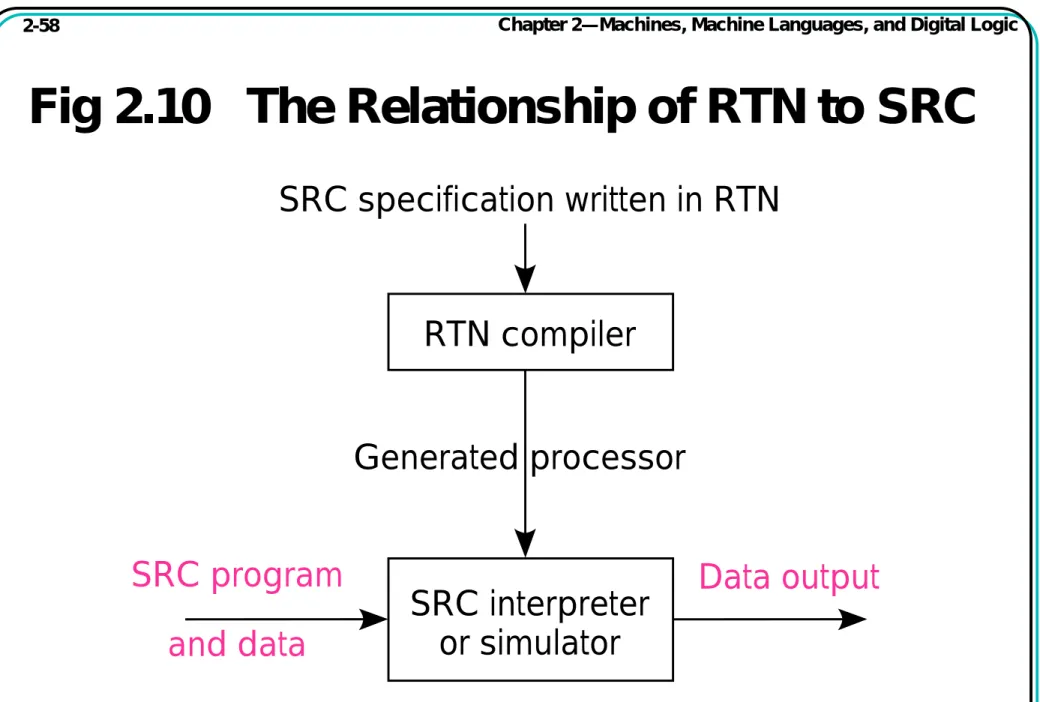
• Other examples: LEX, YACC, VHDL, Verilog Figure 2.10 may help clear this up...

Fig 2.10 The Relationship of RTN to SRC

SRC specification written in RTN

RTN compiler

Generated processor

SRC program

and data

Data output

SRC interpreter

or simulator

A Note About Specification Languages

• They allow the description of what without having to specify how.

• They allow precise and unambiguous specifications, unlike natural language.

• They reduce errors:

• Errors due to misinterpretation of imprecise specifications written in natural language.

• Errors due to confusion in design and implementation—“human error.”

• Now the designer must debug the specification!

• Specifications can be automatically checked and processed by tools.

• An RTN specification could be input to a simulator generator that would produce a simulator for the specified machine.

• An RTN specification could be input to a compiler generator that would generate a compiler for the language, whose output could be run on the simulator.

Addressing Modes Described in RTN

(Not SRC)

Mode name Assembler RTN meaning Use

Syntax

Register Ra R[t] ← R[a] Tmp. Var.

Register indirect (Ra) R[t] ← M[R[a]] Pointer

Immediate #X R[t] ← X Constant

Direct, absolute X R[t] ← M[X] Global Var.

Indirect (X) R[t] ← M[ M[X] ] Pointer Var.

Indexed, based, X(Ra) R[t] ← M[X + R[a]] Arrays, structs

or displacement

Relative X(PC) R[t] ← M[X + PC] Vals stored w pgm

Autoincrement (Ra)+ R[t] ← M[R[a]]; R[a] ← R[a] + 1 Sequential

Autodecrement - (Ra) R[a] ← R[a] - 1; R[t] ← M[R[a]] access.

Fig 2.11 Register Transfers Hardware

and Timing for a Single-Bit Register

Transfer: A

←

B

• Implementing the RTN statement A ← B

Strobe

(a) Hardware

(b) Timing

Strobe

B

A

1

0

1

0

1

0

D

B

Q

Q

D

A

Q

Q

Fig 2.12 Multiple Bit Register Transfer:

A

〈

m..1

〉

←

B

〈

m..1

〉

Fig 2.13 Data Transmission View of

Logic Gates

• Logic gates can be used to control the transmission of data:

Data gate Controlled complement Data merge data gate data control gate→data gate→0 control→data control→data data 1 data1(2), provided data2(1) is zero data 2 data 1 data 2

Fig 2.14 Two-Way Gated Merge, or

Multiplexer

• Data from multiple sources can be selected for transmission x y y x G_x y G_y m x m m m Time

Fig 2.15 Basic Multiplexer and Symbol

Abbreviation

• Multiplexer gate signals Gi may be produced by a

binary to one-out-of-n decoder

D₀ D₁ G₀ G_n–1 D_n–1 m

An n-way gated merge An n-way multiplexer with decoder

(a) Multiplexer in terms of gates (b) Symbol abbreviation

m m m D₀ D₁ m m m D_n–1 m k Select G₁ m m m

Fig 2.16 Separating Merged Data

• Merged data can be separated by gating at the right time

• It can also be strobed into a flip-flop when valid

x

y

G

m

x

m

0

Time

Fig 2.17 Multiplexed Register

Transfers Using Gates and Strobes

• Selected gate and strobe determine which RT

• A←C and B←C can occur together, but not A←C and B←D

G_C S_A S_B G_C Hold time Propagation time S_B m m D C Q Q G_D Gates Strobes m m m m D D Q Q D A Q Q D B Q Q m

Fig 2.18 Open-Collector NAND Gate

Output Circuit

(a) Open-collector NAND truth table

(b) Open-collector NAND (c) Symbol

Fig 2.19 Wired AND Connection of

Open-Collector Gates

(a) Wired AND connection _{(b) With symbols}

(c) Truth table

+V

Fig 2.20 Open-Collector Wired OR Bus

• DeMorgan’s OR by not of AND of NOTS

• Pull-up resistor removed from each gate - open collector

• One pull-up resistor for whole bus

• Forms an OR distributed over the connection

+V D_n–1 G_n–1 D₁ G₁ D₀

Fig 2.21 Tri-State Gate Internal

Structure and Symbol

Data

Enable

(a) Tri-state gate structure (b) Tri-state gate symbol

(c) Tri-state gate truth table

Data

Enable

Out Tri- Out

state +V

Enable Data Output

0 0 1 1 0 1 0 1 Hi-Z Hi-Z 0 1

Fig 2.22 Registers Connected by a

Tri-State Bus

• Can make any register transfer R[i]←R[j]

• Can’t have G_{i = Gj = 1 for i}≠_j

• Violating this constraint gives low resistance path from power supply to ground—with predictable results!

m S₀ m m G₀ R[0] Tri-state bus m S₁ m m m G₁ D R[1] Q Q m S_n–1 m m G_n–1 D R[n – 1] Q Q D Q Q

Fig 2.23 Registers and Arithmetic Units

Connected by One Bus

Combinational logic—no memory Example: Abstract RTN R[3] ← R[1]+R[2]; Concrete RTN Y ← R[2]; Z ← R[1]+Y; R[3] ← Z; Control Sequence R[2]_{out, Yin}; R[1]_{out, Zin}; Z_{out, R[3]in};

Notice that what could be described in one step in the abstract RTN took three steps on this particular hardware R[0]_in Y_in R[0]_out m m m m m m R[0] Incrementer Adder D Q R[1]_in R[1]_out m D Q R[n – 1]_in R[n – 1]_out m D Q Q Q Q W_in W_out m Z_out W D Q Q Z_in Z D Q Q R[1] R[n – 1] D Q Q Y

RTs Possible with the One-Bus

Structure

• R[i] or Y can get the contents of anything but Y

• Since result different from operand, it cannot go on the bus that is carrying the operand

• Arithmetic units thus have result registers

• Only one of two operands can be on the bus at a time, so adder has register for one operand

• R[i] ← R[j] + R[k] is performed in 3 steps: Y←R[k]; Z←R[j] + Y; R[i]←Z;

• R[i] ← R[j] + R[k] is high level RTN description

• Y←R[k]; Z←R[j] + Y; R[i]←Z; is concrete RTN

From Abstract RTN to Concrete RTN to

Control Sequences

• The ability to begin with an abstract description, then describe a hardware design and resulting concrete RTN and control sequence is powerful.

• We shall use this method in Chapter 4 to develop various hardware designs for SRC.

Chapter 2 Summary

• Classes of computer ISAs

• Memory addressing modes

• SRC: a complete example ISA

• RTN as a description method for ISAs

• RTN description of addressing modes

• Implementation of RTN operations with digital logic circuits