Masthead Logo
Nova Southeastern University
NSUWorks
CEC Theses and Dissertations College of Engineering and Computing2019
LSTM Networks for Detection and Classification
of Anomalies in Raw Sensor Data
Alexander Verner
Nova Southeastern University,[email protected]
This document is a product of extensive research conducted at the Nova Southeastern UniversityCollege of Engineering and Computing. For more information on research and degree programs at the NSU College of Engineering and Computing, please clickhere.
Follow this and additional works at:https://nsuworks.nova.edu/gscis_etd Part of theComputer Sciences Commons
Share Feedback About This Item
This Dissertation is brought to you by the College of Engineering and Computing at NSUWorks. It has been accepted for inclusion in CEC Theses and Dissertations by an authorized administrator of NSUWorks. For more information, please [email protected].
NSUWorks Citation
Alexander Verner. 2019.LSTM Networks for Detection and Classification of Anomalies in Raw Sensor Data.Doctoral dissertation. Nova Southeastern University. Retrieved from NSUWorks, College of Engineering and Computing. (1074)
LSTM Networks for Detection and Classification of Anomalies in Raw Sensor Data
by
Alexander Verner
A dissertation submitted in partial fulfillment of the requirements for the degree of Doctor of Philosophy
in
Computer Science
College of Engineering and Computing Nova Southeastern University
An Abstract of a Dissertation Submitted to Nova Southeastern University in Partial Fulfillment of the Requirements for the Degree of Doctor of Philosophy
LSTM Networks for Detection and Classification of Anomalies in Raw
Sensor Data
by
Alexander Verner March 2019
In order to ensure the validity of sensor data, it must be thoroughly analyzed for various types of anomalies. Traditional machine learning methods of anomaly detections in sensor data are based on domain-specific feature engineering. A typical approach is to use domain knowledge to analyze sensor data and manually create statistics-based features, which are then used to train the machine learning models to detect and classify the anomalies. Although this methodology is used in practice, it has a significant drawback due to the fact that feature extraction is usually labor intensive and requires considerable effort from domain experts.
An alternative approach is to use deep learning algorithms. Research has shown that modern deep neural networks are very effective in automated extraction of abstract features from raw data in classification tasks. Long short-term memory networks, or LSTMs in short, are a special kind of recurrent neural networks that are capable of learning long-term dependencies. These networks have proved to be especially effective in the classification of raw time-series data in various domains. This dissertation systematically investigates the effectiveness of the LSTM model for anomaly detection and classification in raw time-series sensor data.
As a proof of concept, this work used time-series data of sensors that measure blood glucose levels. A large number of time-series sequences was created based on a genuine medical diabetes dataset. Anomalous series were constructed by six methods that interspersed patterns of common anomaly types in the data. An LSTM network model was trained with k-fold cross-validation on both anomalous and valid series to classify raw time-series sequences into one of seven classes: non-anomalous, and classes corresponding to each of the six anomaly types.
As a control, the accuracy of detection and classification of the LSTM was compared to that of four traditional machine learning classifiers: support vector machines, Random Forests, naive Bayes, and shallow neural networks. The performance of all the classifiers was evaluated based on nine metrics: precision, recall, and the F1-score, each measured in micro, macro and weighted perspective.
Alexander Verner While the traditional models were trained on vectors of features, derived from the raw data, that were based on knowledge of common sources of anomaly, the LSTM was trained on raw time-series data. Experimental results indicate that the performance of the LSTM was comparable to the best traditional classifiers by achieving 99% accuracy in all 9 metrics. The model requires no labor-intensive feature engineering, and the fine-tuning of its architecture and hyper-parameters can be made in a fully automated way. This study, therefore, finds LSTM networks an effective solution to anomaly detection and classification in sensor data.
Acknowledgments
Several people have guided, supported and encouraged me throughout my journey to pursue a doctoral dissertation from this esteemed institution.
First and foremost, I would like to express my appreciation to Dr. Sumitra Mukherjee, my academic advisor, for his guidance, strategic advice and invaluable comments provided during this challenging endeavor.
I would also like to thank my committee members: Dr. Francisco J. Mitropoulos and Dr. Michael J. Laszlo for encouraging my study and its positive evaluation.
I am most sincerely grateful to my parents, Igor and Marina, and to my brother Uri, for the time they invested in making my work better.
I thank my grandparents, Matvey and Eleonora, for believing in me and supporting my aspirations.
I am grateful to my wife Nadezhda for taking care of all my needs, and my kids Artiom and Polina, for being my source of inspiration along the way.
v
Table of Contents
Approval ii Abstract iii
Acknowledgements iv List of Tables vii List of Figures viii Chapters
1. Introduction 1
Background 1 Problem Statement 3 Dissertation Goal 5
Relevance and Significance 6 Summary 8
2. Literature Review 10
Anomalies as Outliers 10 Anomalies in Sensor Data 13
Taxonomy of Anomaly Detection and Classification Methods 14 Techniques based on Feature Engineering 16
Techniques based on Automated Feature Extraction 19 Existing LSTM-based Solutions 22
Summary 23 3. Methodology 24
Experiment Design 25 Chosen Dataset 29
Data Cleaning and Preprocessing 30
Experiment 1: Classification by Means of SVM 34 Experiment 2: Classification via Random Forest 36
Experiment 3: Classification via Naive Bayes Classifier 39 Experiment 4: Classification via Shallow Neural Network 42 Experiment 5: Classification via LSTM 45
Resources 54 Summary 55 4. Results 56
Results of Dataset Processing 57 Results of Experiment 1 58 Results of Experiment 2 60 Results of Experiment 3 62 Results of Experiment 4 64 Results of Experiment 5 66 Summary 72
5. Conclusions, Implications, Recommendations, and Summary 74
Conclusions 74 Implications 76
vi
Recommendations 76 Summary 78
Appendices 83
A. Detailed Experiment Results 84 B. Third Party Libraries 105 References 107
vii
List of Tables
Tables
1. Table 1. Blood glucose level ranges for different patient groups 30 2. Table 2. Detailed data split by categories 31
3. Table 3. Hand-crafted features for traditional ML algorithms 33
4. Table 4. Random feature vectors, constructed from normal and anomalous sequences 58
5. Table 5. Confusion matrix and full classification report of the best found SVM classifier 59
6. Table 6. Confusion matrix and full classification report of the best-found Random Forest classifier 62
7. Table 7. Confusion matrix and full classification report of the best-found naive Bayes classifier 64
8. Table 8. Confusion matrix and full classification report of the best-found shallow neural network classifier 66
9. Table 9. Confusion matrix and full classification report of the best-found LSTM classifier 71
viii
List of Figures
Figures
1. Figure 1. A multisensor-based noninvasive continuous glucometer 2 2. Figure 2. An example of point anomaly 11
3. Figure 3. Example of contextual anomaly 12 4. Figure 4. Example of collective anomaly 13 5. Figure 5. Design of the planned experiment 28
6. Figure 6. Histogram of JDRF values and their number of appearances 32 7. Figure 7. Using SVM to separate two-dimensional data 35
8. Figure 8. Example of general balanced decision tree 37
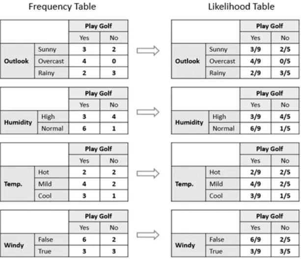
9. Figure 9. Example of majority-voting on the final class in Random Forest 38 10. Figure 10. The process of creation of frequency and likelihood tables,
demonstrated on the Golf Dataset 40
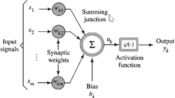
11. Figure 11. Information processing in a single neuron 43 12. Figure 12. Architecture of a typical shallow neural network 44 13. Figure 13. RNN unit - unfolding of events over time 46 14. Figure 14. Architecture of a single ordinary RNN unit 46 15. Figure 15. Architecture of a single unit of vanilla LSTM 48
16. Figure 16. Anomaly detection in 1D web traffic time-series data 52 17. Figure 17. Discrete sequences of measured glucose levels, represented as
continuous curves 57
18. Figure 18. Histograms of four different SVM models’ accuracy scores, measured by nine metrics 59
19. Figure 19. Histograms of four Random Forest models’ accuracy scores, measured by nine metrics 61
ix
20. Figure 20. Histograms of four naive Bayes classifier model’s accuracy scores, measured by nine metrics 63
21. Figure 21. Histograms of four shallow neural network models’ accuracy scores, measured by nine metrics 65
22. Figure 22. Histograms of four LSTM models’ accuracy scores, measured by nine metrics 68
23. Figure 23. Graphs of four LSTM models’ accuracy and loss versus epochs during k-fold cross-validation 69
1
Chapter 1 - Introduction
Sensor validation relies on understanding of several basic concepts, such as the dependence of a sensor-based system on the validity of the data, the relation between various sensor faults and anomalies in the data, the importance of timely detection of the data, etc. This role of this chapter is to familiarize the reader with the field of detection and classification of anomaly in sensor data and explain the essence of the proposed dissertation. The introduction is divided into the following sections:
• Background
• Problem Statement
• Dissertation Goal
• Relevance and Significance
• Summary
Background
Sensors are widely used in industry, daily life and medicine. Wearable or implanted medical devices, such as insulin sensors, have been used for several decades to non-invasively collect electrical, thermal and optical signals generated by the human body (Mosenia, Sur-Kolay, Raghunathan, & Jha, 2017). Vibration, temperature and noise sensors are used in nuclear power plants, gas turbines and continuous stirred-tank reactors, (Luo, Misra, & Himmelblau, 1999; Gribok, Hines, & Uhrig, 2000; Yan & Goebel, 2003). Numerous other examples of complex sensor-based systems that operate on data received from the sensors have been well documented. These observations suggest that, ultimately, the correct functioning of these systems strongly
2
depends on the reliability of sensor data. For instance, Figure 1 (Geng, Tang, Ding, Li, & Wang, 2017) shows a multisensor-based noninvasive continuous glucometer that uses several sensors to measure blood glucose levels:
Unfortunately, sensors often fail. These failures can be caused by a variety of reasons, such as physical damage (both intentional and unintentional), manufacturer defects, software errors, unmonitored environmental conditions, incorrect calibration or configuration, improper human-computer interaction (HCI), misuse, and even hacking and abuse for malicious purposes (Van Der Meulen, 2004; Sikder, Petracca, Aksu, Jaeger, & Uluagac, 2018). When these failures occur, they lead to anomalies appearing in the data, making it permanently unreliable, or in the least, for a certain amount of time. When data with anomalies is fed upstream to high-level processing stages, this often leads to system's incorrect behavior of the system with unpredictable
3
and even dangerous consequences, such as insulin overdose or nuclear plant shutdown. With sensors becoming so ubiquitous and implications of their failure becoming so significant, timely detection of anomaly has also become extremely important. Classification of anomalies is also of high priority, since it helps to identify the root cause of the failure and take relevant preventive actions.
Problem Statement
Detection and classification of anomalies in raw time-series sensors data in a way that does not require domain knowledge is an open research challenge. Until now, the vast majority of existing anomaly detection and classification methods have been based on hand-crafted features (Goldstein, & Uchida, 2016; Parmar, & Patel, 2017;
Yi, Huang, & Li, 2017). These methods require considerable human effort from domain experts and are strongly tailored to specific system design and type of data.
Much scientific effort has been devoted to the subject of sensor data validation and various algorithms of anomaly detection and classification have been proposed for sensor-based systems over the past decades Yao, Cheng, & Wang, 2012; Pires, Garcia, Pombo, Florez-Revuelta, & Rodriguez, 2016). A detailed review of these methods appears in Chapter 2 of this dissertation.
The very first approaches were primitive and mainly involved sensors redundancy in hardware with further majority voting. Due to their high cost, they were soon replaced by a series of approaches that were based on mathematical (mostly statistical) models that spotted errors by quantifying the degree of relationship between the measured distribution and the predicted one.
4
However, over time, sensor-based systems became more complex and included a variety of sensors differing by characteristics, such as type, manufacturer, degree of quality, accuracy, stability, deterioration over time, resistance to noise and external factors (Worden, 2003; Jager et al., 2014). As a result, statistical models became impractical for these multipart systems (Pires et al., 2016), and were replaced by approaches based on classical ML models, such as shallow neural networks (SNN) (Hopfield, 1982), principal components analysis (PCA) (Pearson, 1901), Random Forest (Ho, 1995), etc. Unlike statistical approaches that focus on understanding the process that generated the data, ML techniques focus on constructing a mechanism that improves its accuracy based on previous results (Patcha, Park, 2007).
For more than two decades, various classical ML models have been successfully used to detect anomaly in sensor data (Wise, & Gallagher, 1996; Luo, Misra, & Himmelblau, 1999; Misra, Yue, Qin, & Ling, 2002; Tamura, & Tsujita, 2007; Auret, & Aldrich, 2010; Singh & Murthy, 2012; Jager et al., 2014; Cerrada, et al., 2016;
Zhang, Qian, Mao, Huang, Huang, & Si, 2018). However, despite of their success, ML methods that involve manual feature extraction have two serious shortcomings: firstly, these methods cannot operate on raw data. Instead, they operate on features extracted from the data, which is labor intensive and requires considerable effort from domain experts. To construct them, a domain expert needs to take into consideration the peculiarities of the analyzed sensors to manually control and tune their input (Bengio, Courville, & Vincent, 2013). Secondly, such methods are domain specific. Being tailored to concrete sensor-based systems and concrete type of data, these approaches are highly sensitive to the slightest changes in the system or the data (Ibarguengoytia, 1997).
5
Unfortunately, modern sensor-based systems are very dynamic. Their complexity constantly increases, which requires periodical design changes. The nature of data that these systems rely on is also volatile and often changes. When these radical changes occur, previous feature-based solutions cease to function properly and require fundamental redesign or refactoring, which again results in considerable human effort. These limitations make most of the current methods inefficient and point to the need for an approach that would provide significantly longer-lasting solutions to detect and classify anomalies, do not require domain knowledge, and can be relatively easily adjusted to new system design or new types of data. This is the challenge that makes data anomaly detection in sensor data an unsolved problem that requires further consideration.
Dissertation Goal
This dissertation systematically investigated the effectiveness of long short-term memory networks (LSTMs) (Hochreiter, & Schmidhuber, 1997) for anomaly detection based on raw sensor data. As a proof of concept, it planned to use time-series data on glucose level measurements. Samples of anomalous time-series sequences, generated by using six methods that represent common types of anomaly, were used along with non-anomalous time-series sequences. An LSTM network model was trained on a medical dataset with real data to classify raw time-series sequences into one of seven classes: non-anomalous, and classes corresponding to the six types of anomalies.
The model’s generalization success was estimated by means of k-fold cross-validation (Kohavi, 1995). To evaluate its performance (classification accuracy) a confusion matrix was used to compute precision, recall, and F1 score (F-measure)
6
(Sammut, & Webb, 2017). Each of the three metrics examined in micro, macro and weighted perspective, resulting in a total of 9 metrics. As a control, the performance of the LSTM model, trained on raw time-series data, was compared to performance of traditional classifiers, such as SNNs, support vector machines (SVMs), random forests (RF) (Ho, 1995), and naive Bayes classifier (NBC) that were trained on hand-crafted features based on knowledge about the common sources of anomaly.
Relevance and Significance
As discussed in the Introduction section of this chapter, sensor-based systems are highly dependent on validity of data received from the sensors. Anomalies in sensor data caused by various failures lead to incorrect system behavior with unpredictable and even dangerous consequences. Therefore, precise and timely detection of anomalies and identification of their types is of extreme importance.
As previously mentioned, former methods, as well as vast majority of recent ones, operate on hand-crafted features, which results in significant limitations, such as considerable human effort and lack of resilience to changes in system or underlying data. It is clear that an alternative approach to anomaly detection and classification that would be able to process raw data and automatically generate the required features will be particularly valuable. One method that meets these requirements is LSTM. Research has shown that this contemporary ML model is very effective in automated extraction of abstract features from various raw time-series (Salehinejad, 2017). Moreover, LSTM is capable of learning long-term dependencies from sequential and time-series data (Dam et al., 2017; Karim, Majumdar, Darabi, & Chen, 2018). As a result, solutions based on LSTM have several substantial benefits:
7
- They remove the necessity for a domain expert. - They significantly reduce human effort.
- They decrease design complexity.
- They automatically adjust to new types of data. - They will have longer lifespans.
- They are automated to a large extent and require significantly less calibration to address concrete problems.
For reasons that remain unclear, LSTM is little used in anomaly detection and classification. This model has existed for over twenty years, but solutions based on LSTM have only started to appear in recent years (Pires et al., 2016; Parmar, & Patel, 2017). A thorough search through recent survey papers revealed that the number of proposed LSTM-based systems for anomaly detection in raw sensor data is negligible in comparison with systems based on feature engineering. These facts indicate that there is no confidence in the research community that LSTM is a promising approach for anomaly detection in raw time-series. However, despite the absence of proper recognition and attention from the research community, the aforementioned benefits of LSTM make it an extremely well-suited method for the above task.
Previous experimental supports this claim. For instance, Fehst, Nghiem, Mayer, Englert and Fiebig (2018) compared techniques based on manual feature engineering and feature subset selection for dimensionality reduction with automatic feature learning through LSTM. The results of their study show that LSTM has significantly higher accuracy. Other works (Chauhan, & Vig, 2015; Malhotra, Vig, Shroff, & Agarwal, 2015; Taylor, Leblanc, & Japkowicz, 2016; Yoshikawa, Belkhir, & Suzuki, 2017; Zhang, & Zou, 2018) have also reported on the successful use of LSTM for solving practical anomaly detection problems in domains such as medicine,
8
automotive, power, aviation, etc. In his master’s thesis, Singh (2017) claims that LSTMs are suitable for general purpose time-series modeling and anomaly detection and proves this by successfully applying the model on three real-world datasets from different domains. There are other works as well; the complete list appears in the
Existing LSTM-based Solutions section of Chapter 2.
The proposed research considers the effectiveness of LSTM in modeling time-series of raw data, and its abilities of the capturing long range dependencies. It takes into account the full compatibility of the above qualities to the field of application, i.e. anomaly detection and classification in sensor data. Finally, it relies on the optimistic experience of and impressive results of existing works that recommended LSTM-based solutions. These three factors combined constitute a well-founded motive to consider further investigation of this pertinent and important approach.
While the proposed dissertation deals with a practical problem of detecting sensor faults, it also aims to contribute to the knowledge base of computer science. The study deals with the application of ML methods for analyzing sensor data and may provide new directions and ideas for the effective application of these methods. Particularly, the study is expected to contribute to an LSTM-based approach in the analysis of medical-sensor data. Finally, evaluation of the extent in which LSTM can replace approaches based on feature engineering will contribute to the study of the effectiveness and practical value of this model.
Summary
This chapter begins by providing some background information in anomaly detection. It introduces multi-sensor systems and their dependency on valid sensor
9
data. It discusses the problem of sensors failures that cause anomaly in the data, and the importance of its timely detection and classification. The chapter then continues with a brief overview of existing methods, explains their dependence on manual extraction of features from the data, and the problem imposed by these limitations in light of complex and constantly changing modern systems. Next, the chapter defines the goal of the proposed dissertation: systematic investigation of the effectiveness of LSTM for anomaly detection based on raw sensor data and clarifies how it can be achieved by the planned study experiment. Finally, this chapter positions the importance of precise and timely detection of anomalies and identification of their types. It emphasizes the benefits of the LSTM model, its effectiveness and accuracy, and the its resulting eminent appropriateness as a method for detection and classification of anomaly in sensor data. These claims are justified by mentioning several relevant works of research. Finally, the chapter elaborates on the contribution of the proposed dissertation to the knowledge base of computer science.
The remainder of this dissertation proposal is organized as follows: Chapter 2 provides literature review on types of anomaly, detection and classification methods, feature engineering and others. It serves as the baseline and starting point of the research. Chapter 3 presents the methodology of the investigational portion of the study. It presents a detailed experiment design, choice and dataset preprocessing, and each of the five stages of the planned experiment. Chapter 4 shows the results of the experimental part of the study. Chapter 5, the last one in this dissertation, concludes results of the investigation and draws inferences from them.
10
Chapter 2 - Literature Review
The primary focus of this dissertation’s research is detection and classification of anomaly in sensor data. There is a considerable research-community interest in this area. The following sections review the relevant literature:
• Anomalies as Outliers
• Anomalies in Sensor Data
• Taxonomy of Anomaly Detection and Classification Methods
• Techniques based on Feature Engineering
• Techniques based on Automated Feature Extraction
• Existing LSTM-based Solutions
• Summary
Anomalies as Outliers
Invalid data differs from valid data by the fact that it contains a certain amount of anomalous values that are discordant observations and do not conform to expected behavior (Hayes, & Capretz, 2014). Statistically, anomalies can be referred to as outliers in baseline distribution of the data or of its features (Stoecklin, 2006). Therefore, in the context of data validation, failure localization and recognition are equivalent to detection and classification of outliers. Anomalies can be classified into the following four categories (Parmar, & Patel, 2017):
1. Point anomaly. These are individual data points that are considered anomalous with respect to the remaining data. This type of anomalies refers to data points that
11
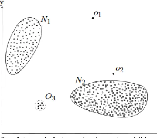
are given without contextual aspect, such as time. Figure 2 (Chandola, Banerjee, & Kumar, 2009) shows an example point anomaly in a 2D dataset:
As seen in the Figure, most observational data points reside within the two regions
1
N and N2. This data in these regions can be considered normal. On the contrary, points o1 and o2, and region O3 are anomalous. They are sufficiently distant from the normal regions, which makes them outliers.
2. Contextual anomaly (also called conditional anomaly). These are individual data points that are anomalous in a specific context, but not otherwise. The context is defined by the structure of the dataset and is problem specific. Each data point is defined by attributes that define the neighborhood (context) of the point, and behavioral attributes that express its non-contextual characteristics. When dealing with time-series data, such as the one examined by this work, an outlier is defined
Figure 2. An example of point anomaly: points o1 and o2, and all the points within the region O3 are outliers.
12
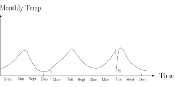
as a data point that must have both contextual anomaly and behavioral anomaly. In other words, it must have anomalous values that appear within an anomalous context. Figure 3 (Chandola, Banerjee, & Kumar, 2009) shows an example of contextual anomaly in a 1D time-series data of temperature over the year:
Points t1 and t2 have about the same low values. On the one hand, t1 is considered
normal since it stays within the climatic norm for the period of December to March. On the other hand, t2 is an outlier, since such low temperatures is not
expected in June. It is plain to see that the time context (months in this example) affect the normality of the data.
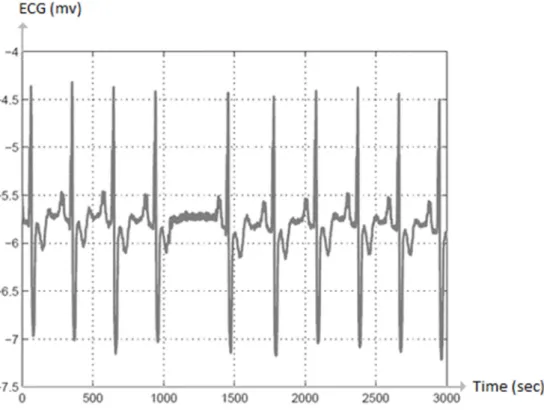
3. Collective anomaly. This type of anomaly refers to a collection of related data points, which are anomalous with respect to the entire dataset. Two notes are worth mentioning: firstly, individual data points in such an anomalous collection may not be anomalies by themselves, while only their common existence shows up as anomaly. Secondly is that this type of anomaly can appear in both context-aware data and contextless data. Figure 4 (Chandola, Banerjee, & Kumar, 2009) shows an example of collective anomaly in data from an ECG sensor:
13
Each individual data point in the close-to-zero section between 1000 and 1500 seconds is not an anomaly by itself - as seen on the graph that the curve of the periodic oscillations crosses zero value several times. However, if the number of subsequent low-value points is large enough, then they appear to be an anomaly as a group (in this case a premature atrial contraction, PAC).
Anomalies in Sensor Data
As previously mentioned, timely validation of raw sensor readings is critical to prevent invalid data from causing damage to the system, both detection and classification of invalid data are equally important. Whereas the first protects the system from being damaged by invalid sensor data readings, the second allows the nature of the fault to be understood and allow relevant corrections and improvements to be made in the sensor's system to prevent future reappearances (Scherbakov,
14
Brebels, Shcherbakova, Kamaev, Gerget, & Devyatykh, 2017). A detailed review of data correction methods, given by Pires et. al. (2016), is beyond the scope of this work. The task of outlier detection and classification is especially multifaceted and challenging when sensor data is concerned, and stems from the following factors (Chandola, Banerjee, & Kumar, 2009):
1. The boundary between normal and anomalous behavior is often not precise. Anomalous observations may lie very close to normal, and vice-versa, which makes it very difficult to define a region with every possible normal behavior. 2. When anomalies originate from malicious actions, they appear as normal sensor
data, making it very difficult to define normal behavior.
3. A defined notion of normal behavior that was sufficiently representative at some point in time may stop being credible later. In many domains the normal behavior dynamically evolves as the system collects new data. Therefore, applying a technique of one specific domain to another is not often impractical.
4. When machine learning (ML) based anomaly methods are used, labeled data for training and validation of models is often a major issue.
5. The data is often interspersed with noise which tends to be quite similar to the actual anomalies. It is very difficult to distinguish and remove such noise.
Taxonomy of Anomaly Detection and Classification Methods
Through the course of history many scientists and researchers have devoted their time to the problem of detection and classification of anomaly in sensor data. One of the simplest sensor failure detection methods is to use multiple sensors of the same type, then compare the readings and decide by majority-voting which, if any, of them
15
are damaged. Not to mention the fact that this redundancy method cannot classify the anomaly, it sometimes fails to detect the anomaly, e.g. if an environmental factor, such as noise, affects the values of all sensors.
Obviously, more advanced and generic methods were needed to serve complex sensor-based systems and started to appear as early as in the 19th century (Edgeworth, 1887). Researchers have formulated the problem of outlier detection and classification by adopting concepts from various disciplines, such as statistics, information theory, spectral theory, ML and data mining (Chandola, Banerjee, & Kumar, 2009). These formulations were based on model of normal data patterns and generation of outlier score for each new data sample. The following types of models have been suggested (Aggarwal, 2015):
1. Extreme values-based models. These models use boundary values to define the range of normal data. Outliers are data points that exceed these boundaries. Data points can be univariate as well as multivariate.
2. Clustering-based models. These models create clusters of data points that occur together. Outliers are data points that appear far away from the clusters.
3. Distance-based models. These models use the distribution of total distance from each data point to its k-nearest neighbors. For an outlier, this distance is significantly larger than for other data points.
4. Density-based models. These models use the local density of the data points. Outliers have low density.
5. Probability-based models. Similar to clustering-based models, these models create data points clusters. However, instead of using distance to determine outlier score, it is determined by the probabilistic fit of a data point.
16
6. Information-theoretic models. This type of model is significantly different from the previous ones. When constructing a normal data model, its space requirements are analyzed. Then, for each new point, the difference on space requirements between construction of a normal model with or without this data point is examined. If the difference is large, the point is reported as an outlier.
These models produced many techniques to anomaly detection and classification that can be grouped into three fundamental approach types (Hodge, & Austin, 2004): 1. Type 1. Techniques that detect the outliers with no prior knowledge of the data. In
ML, these are unsupervised clustering methods. The models are constructed by processing all data, while the most distant points are marked as potential outliers. 2. Type 2. Techniques that are based on labeled data. This approach models both
normal and abnormal data and uses supervised learning-based classification. 3. Type 3. Techniques of this type label only normal data. In this approach, also
known as novelty detection or novelty recognition, semi-supervised ML algorithms, that are trained on the normal data, learn to recognize abnormality patterns by comparing them to those previously seen.
Techniques Based on Feature Engineering
In feature engineering, domain knowledge is used to analyze the raw data and process it to create informative hand-crafted features, which are then used to train the machine learning models. Below is a list of various feature-based methods, based on the works of Patcha and Park (2007), Yao et al. (2012), and Pires et al. (2016):
1. Profile-based behavioral analysis. The idea behind this method is to use hand-crafted features to create a profile of data that is considered normal. This profile
17
then serves as a gauge of valid data patterns. If new data significantly deviates from the profile, it is considered anomalous. A set of rules determines the conditions that trigger the detection of an outlier. This could be a significant deviation of a certain critical feature, a combination of important features, or a common deviation score. The work of Branisavljevic, Kapelan and Prodanovic (2011) used this method to create a real-time data anomaly detection scheme.
2. Bayesian network techniques (Friedman, Geiger, & Goldszmidt, 1997). This approach is based on a model that analyzes and encodes relationships of features in a dataset in a form or directed acyclic graph (DAG). The encoded relationships can be either casual or probabilistic, whereas the features are often chosen to be statistical. For a new sample, the model estimates its probabilistic behavioral likelihood, and decides whether it is normal or an outlier. Kruegel, Mutz, Robertson and Valeur (2003) applied this technique in a multi-sensor system for classification and suppression of false alarms.
3. PCA and clustering techniques. PCA (Pearson, 1901) significantly compresses dataset representation by converting data from the original feature space into a reduced one. The method preserves most of the information by leaving just a few principal components - linear combinations of original features that maximize the variance. After applying PCA, the clustering phase starts. Some metrics, e.g. Canberra, is applied to the normal part of the data to compute a centroid in the new feature space. The distance of new samples from the normal data centroid is large for anomalous samples and small for normal ones. This approach was used by Shyu and Chen and Sarinnapakorn and Chang (2003) in an unsupervised learning scheme for intrusion detection.
18
4. Inductive rule generation techniques (Quinlan, 1987). This approach derives a set of association rules and frequent patterns from the train set. Each rule implies the category (either normal or anomalous) of the target variable by a range of feature values. For example, Decision Trees (DTs) (Quinlan, 1986) implement generate impurity measures-based rules generation. Bombara, Vasile, Penedo, Yasuoka and Belta (2016) used custom rule generation scheme in DT to detect and classify anomalies in data of maritime environment and automotive powertrain system. 5. Fuzzy logic techniques (Novak, Perfilieva, & Mockor, 2012). This approach
analyzes the features and builds a set of fuzzy rules that describe behavioral patterns of normal data, which are then used to form intervals of normal and anomaly data. For new samples, the rules determine whether they fall inside a normal interval or in one of the anomaly intervals. Linda, Manic, Vollmer, and Wright (2011) have proposed a fuzzy logic-based algorithm anomaly detection and classification in network cyber security sensors.
6. Genetic algorithms (GAs) (Whitley, 1994). Originally these evolutionary algorithms used mutation, crossover and selection operators to find solutions for optimization and search problems. However, due to their flexibility and robustness, they have been adjusted for other uses. One adaptation is to use a GA to derive highly effective classification rules. Another is to use GA to select an effective subset of features for other ML algorithms. Both customization methods have been put into practice in detection and classification of anomaly in network traffic (Hassan, 2013; Chouhan, & Richhariya, 2015).
7. Traditional ML models. This approach uses traditional ML models, such as SNNs, SVMs (Cortes, & Vapnik, 1995), RFs (Ho, 1995), and NBCs (Rish, 2001) data. When traditional ML models are used, anomaly detection and classification is
19
carried out as supervised learning task. For instance, Gribok, Hines and Uhrig (2000) have used an SVM to validate labeled nuclear reactor sensor data.
Techniques Based on Automated Feature Extraction
ML algorithms based on feature engineering show excellent results. However, as previously mentioned, manual creation of the features is both domain specific and labor intensive. The accuracy of classification that relies on feature engineering largely depends on how well the hand-crafted features are constructed (Bengio, Courville, & Vincent, 2013). To cope with these shortcomings, recent research is directed to find models that are capable of automated feature extraction (Salahat, & Qasaimeh, 2017). An exhaustive literature search (Hodge, & Austin, 2004; Chandola, Banerjee, & Kumar, 2009; Chandola, Cheboli, Kumar 2009; Parmar, & Patel, 2017; Heaton, 2017;
Fehst et al., 2018) reveals several types of approaches that use automated feature extraction, also known as automated feature engineering and automated feature learning:
1. Fuzzy logic-based approach. Recently, methods that use fuzzy logic have been extended to automate the production of association rules. Modern fuzzy-logic-based methods use sliding window method to divide the time-series into portions (subsequences). Further, an algorithm of the fuzzy logic inheritance system analyzes these subsequences, looking for general patterns in their shape and amplitude. Since the analysis is carried out in an automated way, these patterns serve as the automatically created features for subsequence. The algorithm also automatically produces a set of association rules that define the order of appearance, mutual dependency relations and other characteristics of internal
20
associations. Izakian and Pedrycz (2013) have used fuzzy-logic to detect anomalies in precipitation measurements and arrhythmia ECG signals.
2. Genetic programming-based approach. In traditional ML, GP methods have been used to select an effective subset of features to reduce the cost of computation during the classification process and improve its efficiency. These methods have been recently significantly enhanced and awarded new capabilities. The first is the ability to derive (synthesize) new features from existing ones; another is to derive new features directly from raw data. Both abilities assume no prior knowledge on the probabilistic distribution of the data, which allows GP methods to be used for automated feature extraction. Guo, Jack and Nandi (2005) have used GP-based technique to detect and classify faults in raw data of vibration rotating machine. 3. Deep feedforward neural networks-based approach. When the dataset is large
enough, special types of neural networks can be used for automated feature extraction. Two types of networks have been used for detection and classification of anomaly in raw data:
A. Self-organizing map (SOM) (Kohonen, 1990). These are competitive learning algorithms for classification problems that do topological mapping from the input space to clusters. To be more specific, SOMs find statistical relationships between data points in a high dimensional space and convert them to geometrical relationships in a two-dimensional map formed by the output neurons. Recent enhancements allowed SOMs to automatically extract important features from raw input data and store them in a structure that preserves the topology. The weight vectors of the output neurons serve as prototypes of the data points and as centroids of clusters of alike data points.
21
Barreto and Aguayo (2009) have used several variations of SOM to detect anomalies in data of a solenoid sensor in NASA’s hydraulic valve.
B. Radial basis function (RBF) neural networks (Lowe, & Broomhead, 1988). A classical RBF network is a three-layer feedforward neural network in which hidden layer nodes use RBF as a nonlinear activation function. The hidden layer of an RBF network performs a nonlinear transformation of the input, whereas its output layer maps the nonlinearity into a new space. RBF optimization is linear and is carried out by adjusting the weights to minimize the mean square error (MSE). Improvements made by Lowe and Tipping (1997), Karayiannis and Mi (1997), and Rojas et al. (2002) allowed to extract features from an RBF network and resize the network as required, making it possible to use the RBF networks with time-series, e.g. to detect novelty elements (Oliveira, Neto, & Meira, 2004).
4. Recurrent neural networks (RNNs) (Bengio, Simard, & Frasconi, 1994). An RNN is comprised of multiple copies of the same modules, each being a neural network that passes a message to its successor. RNNs have two inputs: the present and the recent past. Each recurrent module serves as a memory cell. This makes RNNs perfectly suited for ML problems that involve analysis of sequential data with temporal dynamics, such as time-series data of a sensor. Weights are applied to both current and previous input and can be adjusted by the RNN gradient descent and backpropagation through time (BPTT) (Werbos, 1988). RNNs can operate on raw data and do not require hand crafted features. Like deep feedforward neural networks, they learn appropriate feature representations in their hidden layers (Lipton, Berkowitz, & Elkan, 2015). An ordinary RNN has short-term memory, which means that it can only catch time dependency in rather short sequences of
22
data. To overcome this limitation, two special types of RNNs have been invented: long short-term memory (LSTM) and gated recurrent unit (GRU) (Cho et al., 2014). Both have more complex (gates-based) architecture of each recurrent module, which lets them more accurately maintain memory of important correlations and analyze much longer sequences. In LSTM, the architecture of each recurrent module is more complicated and uses more gates, whereas a GRU module exposes the full hidden content without taking control over the flow of data. As a result, LSTM is more powerful, while GRU is computationally more efficient (Chung, Gulcehre, Cho, & Bengio, 2014). Shipmon, Gurevitch, Piselli and Edwards (2017) have used ordinary RNNs, LSTM and GRU to detect anomaly in time-series data of network traffic.
Existing LSTM-Based Solutions
Since this dissertation focuses on LSTM, it is worth mentioning existing work on the subject of detection and classification of anomaly in time-series data. During the last few years, various LSTM-based solutions have been proposed by the research community to detect anomaly in time-series data from various domains, such as medicine (Chauhan, & Vig, 2015), space (Hundman, Constantinou, Laporte, Colwell, & Soderstrom, 2018), automotive (Taylor, Leblanc, & Japkowicz, 2016), power (Malhotra et al., 2015), astronomy (Zhang, & Zou, 2018), web traffic (Kimа, & Cho, 2018), machinery (Singh, 2017), economy (Ergen, Mirza, & Kozat, 2017), etc.
An especially interesting piece of research was carried out by Fehst et al. (2018). Similar to this dissertation, the authors used LSTM to detect anomaly in time-series data of sensors that measured drinking-water quality. LSTM’s automatic feature
23
learning was compared to a traditional ML method called logistic regression, which used manually prepared features. Experiment results (F1-score) show that LSTM classification quality was superior to that of the traditional approach.
Summary
This chapter began by the describing anomalies as outliers and reviewed several types of the latter. It then observed the peculiarities of detecting anomaly in sensor data. The chapter continued by examining main anomaly detection and classification techniques based on both feature engineering and automatic feature extraction. The chapter ended by listing a number of LSTM-based solutions to anomaly detection in time-series data in multiple domains. The next chapter refers to methodology of the proposed dissertation.
24
Chapter 3 - Methodology
The proposed dissertation investigates the use of LSTM model for the problem of anomaly detection in sensor data. Sensor data can be seen as a time-series, while, as previously mentioned, LSTMs are well-suited for finding difficult patterns in the shape and amplitude of this kind of data. In addition, LSTMs are capable of automatically extracting features from raw time-series data. Therefore, the choice of model in this work can be considered convenient for this task. In order to control the LSTM and estimate its abilities of automated feature extraction, the same problem was solved using several traditional ML algorithms that operated on hand-crafted features. The following ML methods have been selected: SVM, Random Forest, naive Bayes classifier, and shallow neural network. Since this work focuses on sensor data, all five algorithms were trained and tested on a dataset that contains sensor measurements. To realistically demonstrate both experimental approaches, the dataset was carefully chosen.
This chapter describes the planned experiment in the following sections:
• Experiment Design
• Chosen Dataset
• Data Cleaning and Preprocessing
• Experiment 1: Classification via SVM
• Experiment 2: Classification via Random Forest
• Experiment 3: Classification via Naive Bayes
• Experiment 4: Classification via a Shallow Neural Network
25
Experiment Design
Below are the design decisions for each stage of the experimental work:
1. Choosing a dataset. A dataset must be carefully selected to match the goal, scope and facilities of the experiment (LaLoudouana, Tarare, Center, & Selacie, 2003). For the proposed study, the following of dataset requirements have been devised: a. The dataset must contain measurements of real sensors, and have sufficient data
for both training and testing.
b. The dataset should be well-balanced, having each class represented by roughly the same number of samples.
2. Preprocessing the data. The data may suffer from phenomena such as clearly illegal values, missing values, incomplete samples etc. In this case it needs to be cleaned or completed. E.g., in cases where anomalous samples are missing these samples need to be generated and added to existing data. Finally, the data needs to be adjusted to the specific experiments. In case of the proposed work, the samples need to be converted to feature vectors and time-series.
3. Choosing the classifiers. As previously mentioned, anomaly detection and classification should be carried out by using ML algorithms of two types. The first is based on traditional feature-based ML algorithms, namely SVM, RF, NBC and SNN. The second type, an LSTM network, should operate on raw time-series and automatically extract features. Altogether, five classification experiments are to be conducted. First four experiments estimate anomaly detection and classification abilities of the traditional ML models. These models should be trained and validated on feature vectors that were prepared during the dataset preprocessing phase. The fifth classification experiment estimates the ability of LSTM to
26
automatically extract features from raw time-series data and use this knowledge to detect and classify the anomaly. Due to wise construction of statistical domain knowledge-based features, the simpler algorithms can achieve very high classification accuracy. To assess the benefits of LSTM, its accuracy should be matched to that of the traditional models.
4. Training and cross-validating the classifier. One of the main requirements of ML is to build a computational model with both high prediction accuracy and good generalization abilities (Mitchell, 1997). Improperly trained model memorizes the training examples and overfits, resulting in poor generalization on unseen data. To train a good model the bias-variance tradeoff (Kononenko, & Kukar, 2007) should be considered, i.e. the right balance between good prediction on training data and good generalization of new data needs to be found. Cross-validation (CV) (Picard, & Cook, 1984) is considered a conventional approach to ensure good generalization and prevent overfitting. k-fold CV is a slightly more effective (Reitermanova, 2010) variation of CV that also automates the process of dataset partitioning. To keep the models of this study robust and resistant to overfitting, each they should be trained through 10-fold CV.
5. Tuning the classifiers. Tuning a model’s architecture and hyperparameters can significantly improve its accuracy. This type of optimization relies less on theory and more on experimental results. Following the work of Bergstra and Bengio (2012), this study should apply two most popular strategies for hyperparameter optimization: automated grid search and manual search. For traditional ML models that require significantly less time to train, grid search through 10-fold CV will be used to find the best combination of architecture and hyperparameters. To prevent overfitting, the models should be trained through cross-validation. For the LSTM
27
the long training times require manual search of the optimal setup. However, the LSTM should be also trained through 10-fold CV.
6. Testing the model. After being trained, cross-validated, and tuned, the model’s accuracy should be tested. To ensure credible testing, the JDRF dataset should be split in a way called train-cross-validate-test, following the recent trend (Kuhn, 2013). This method splits the data into two parts with ratio of 0.9. Training and cross-validation data is used for training of the model and finding the best set of hyperparameters via k-fold CV, while the testing data is used for testing.
7. Evaluating the model. In order to keep the evaluation results trustworthy and ensure that the accuracy is measured from every angle, this study should follow the recommendations of Goutte and Gaussier (2005). Once tested, a confusion matrix should be constructed from computed true positives (TP), true negatives (TN), false positives (FP) and false negatives (FN) test results. Then, the following nine metrics should be computed: micro-precision, macro-precision, weighted precision, micro-recall, macro-recall, weighted-recall, micro-F1 score, macro-F1 score, and weighted F1-score. In LSTM, there should be another two metrics: the interrelations between accuracy and loss of the model, and the number of epochs elapsed during the training process. This will allow to estimate the effectiveness of the model apart from its accuracy.
8. Reasoning on LSTM’s advantages. Estimation of the algorithms' classification accuracy should serve as the quantitative analysis that is required to examine its effectiveness. By comparing the overall classification results of the traditional ML algorithms with the LSTM, it should possible to discern if the expected results in automated feature engineering have been achieved and if the LSTM can be used as a preferable alternative to classical models in the domain of sensor data.
28 Feature vectors Time-series Original dataset Cleaning Completing
Train data Validate data
Fold 1 Fold 2
Validate
data Train data Fold k
Splitting to train-validate-test data
LSTM classifier
Creating, training and tuning best hyperparameters on k-fold CV data
Evaluation of test data, computing precision, recall and F1-score
Experiment results
Generalizing and summarizing Transforming Transforming
Figure 5. Design of the planned experiment.
k-fold CV data Test data
. . .
Train data Validate data Train data
All data
Prediction results Train data Validate data
Validate
data Train data
Traditional ML classifiers
Creating, training and tuning best hyperparameters on k-fold CV data
Evaluation of test data, computing precision, recall and F1-score
k-fold CV data Test data
. . .
Train data Validate data Train data
All data
Splitting to train-validate-test data
Prediction results
29
9. Generalizing and summarizing the experiment results. The experiments should provide sufficient "food for thought" from their results to facilitate the addressing of the following questions:
• What is the meaning behind the achieved results?
• Could these results be foreseen?
• Would the results have been roughly the same if another dataset was used?
Figure 5 visualizes the phases of the planned experiment. It can be seen that the flow of the traditional ML algorithms and the flow of the LSTM are very much alike. The only difference is the type of data they are applied on. This aspect keeps the experiment straightforward, equitable and precise.
Chosen Dataset
For the proposed dissertation, the Juvenile Diabetes Research Foundation (JDRF) Continuous Glucose Monitoring (CGM) Clinical Trial dataset (JDRF CGM Study Group, 2008) was chosen. This dataset contains genuine measurements of blood glucose levels, which deserve to be called sensor data since blood glucose meters and similar devices are sensor-based. An analysis of the chosen dataset both quantitative and qualitative (Verner, & Butvinik, 2017) revealed that its data is heterogeneous, inconsistent, partially complete and has uneven number of measurements per day. Such data is highly realistic and is expected to provide veridical experiments.
The clinical population examined to prepare the dataset consisted of both healthy people and patients suffering from intensively-treated type 1 diabetes and glycated hemoglobin (HbA1c). Patients were divided into three age groups (over 25 yrs., 15-24
30
yrs., 8-14 yrs.). The measurement period for every patient was about 26 weeks. Table 1 (Verner, & Butvinik, 2017) shows blood glucose level ranges for the patient groups:
Group Age
Glucose Level Range in mg/100 ml
Fasting 1 r. After Meal
2 hr. After Meal Normal w/o Diabetes 11-61 <90 <140 <110 Obese w/o Diabetes 14-62 <90 <140 <110 Normal w/ Diabetes 24-69 80-120 >170 >140 Obese w/ Diabetes 15-65 80-150 >170 >140
The total number of samples in the dataset was 772,061 samples, which is sufficient amount of diverse data to train and test both traditional ML algorithms and LSTM.
The chosen dataset had a couple of issues. First, it contained only normal data and no anomalous samples. This problem was solved by manually generating anomalous data with different types of anomaly from the original data. Another problem was that the data was in rather inconvenient form of numbered measurements with patient IDs and timestamps. The solution was to regroup the data in a way that provided both feature vectors and time-series. The next section covers the details of these procedures.
Data Cleaning and Preprocessing
The dataset was reorganized in a way that placed all subsequent daily measurements of a single patient as a time-series. Since the number of measurements per day differed by both dates and patients, this produced a large amount of variable length time-series. Several series appeared to be too short due to missing or corrupted data. These series provide an insufficient amount of information to be analyzed when detecting outliers and were, therefore, deleted from the dataset. After cleaning out the short time-series,
31
the dataset had 3,826 normal time-series left. Based on the normal sequences, six anomalous time-series were created by embedding different anomalous elements into the normal series. The following six patterns of anomaly were used:
1. Random numbers of extremely large, or extremely small values.
2. Chaotic subsequences of arbitrary length, in which elements significantly and unexpectedly vary from one another.
3. Exorbitantly long subsequences with constant value. 4. Unusually large number of appearances of certain value.
5. Excessively long subsequences of strictly increasing or decreasing values. 6. Excessively long subsequences of two alternating elements.
This resulted in 3,826 x 7 = 26,782 time-series, each labelled by its anomaly type. As previously mentioned, 90% of the data was devoted to training with 10-fold cross-validation, where the remaining 10% were used for testing. Table 2 specifies the number of samples in each category:
Such amount of data was sufficient amount for both traditional and deep ML. The necessary data for the LSTM was prepared. However, to properly finish the transformation phase it was required to convert each time-series into a corresponding
Category Number of
Samples Training with cross-validation - Fold 1 2410 Training with cross-validation - Fold 2 2410 Training with cross-validation - Fold 3 2410 Training with cross-validation - Fold 4 2410 Training with cross-validation - Fold 5 2410 Training with cross-validation - Fold 6 2410 Training with cross-validation - Fold 7 2410 Training with cross-validation - Fold 8 2410 Training with cross-validation - Fold 9 2410 Training with cross-validation - Fold 10 2413
Testing 2679
24103
26782
32
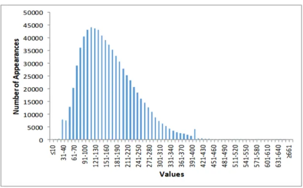
feature vector, to be used by traditional ML algorithms. To prepare a small number of precise and informative features, this study analyzed the nature of the data and used the available domain knowledge. Blood glucose levels act as a bounded curve that fluctuates over time, which is typical for sensors that measure physical quantities. One important task was to find the boundaries of the data. Figure 6 (Verner, & Butvinik, 2017) shows a histogram of the values and their number of appearances:
As seen in the Figure, the JDRF dataset contains both extremely low and extremely high values, such as 19 and 471 mg/dL. Since higher values are occasionally inherent to the human body, it was decided to extend the valid range to [19, 800] mg/dL.
The distribution form has asymmetric Gaussian distribution, which is known to be well described by statistical functions (Gupta, Nguyen, & Sanqui, 2004). The latter implies that manually created features should have statistical nature. In recognition of this fact and the domain knowledge on the types of anomaly, this study proposes eight statistical features that were manually created to estimate the boundaries, averages, deviations and fluctuation patterns of sensor data to identify the six anomaly types.
33
Each feature operates on a single time-series of an arbitrary length (yet, long enough to be left in the dataset). Taken altogether, the features form a (labeled) feature vector of fixed length. Table 3 describes these features and the anomaly types they identify:
Feature Verbal Description
Feature Mathematical Description Identified Anomaly Patterns Minimal value ( )1 ( )2 ( ) ( ) 1
,
,...,
i x i T i if
=
MIN x
x
x
1 Maximal value ( )1 ( )2 ( ) ( ) 2,
,...,
i x i T i if
=
MAX x
x
x
1 Maximal absolute difference between adjacent elements ( ) ( ) ( ) ( ) ( ) ( ) 1 1 1 4 | : i k i k i k i k i j i j x x x x f x j k x − − − = − ∀ ≠ − ≥ − 2 Ratio of maximal number of succeeding repetitions of a constant element to the overall sequence length ( ) ( ) ( ){
}
( ) 1 1 5 | : i k i k ... i i j x k j MAX j k x x x f T + + − ∃ = = = = 3 Mode frequency ( )(
)
( )(
)
(
( ))
3 | : i k i k i j f C x x COUNT j k OUNT COUNT x = ∀ ≠ > 4 Ratio of length of the longest sequence of strictly increasing succeeding elements to the overall sequence length ( ) ( ) ( ){
}
( ) 1 1 7 | : i k i i k x k i j j MAX j k x x x f T + + − ∃ < < … < = 5 Ration of the length of the longest ( ) ( ) ( ){
}
( ) 1 1 7 | : i k i i k x k i j j MAX j k x x x f T + + − ∃ > > … > = 5 Table 3. Hand-crafted features for traditional ML algorithms.34 sequence of strictly decreasing elements to the overall sequence length Length of the longest sequence with two alternating constant elements ( ) ( ) ( ) ( ) ( ) ( ) 1 2 2 2 2 1 3 2 9 1 | , , : j i k j i k i k i k i k i k j j k l m l m f MAX l x x x m x x x − + + + − + + ∃ ≠ ∧ = = = = … = ∧ = = = … = 6
Verner and Butvinik (2017) trained an SVM on the features extracted from the JDRF data that were much like those discussed above. Their model achieved 100% precision and 99.22% recall in binary classification of the data to anomalous and valid. These results were sufficient evidence to assume that if thoughtful hand-crafted features will be used, traditional ML models will be able to achieve high accuracy in anomaly detection and (multiclass) classification.
Experiment 1: Classification via SVM
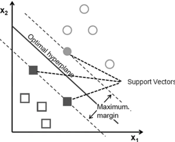
Support vector machine (Cortes, & Vapnik, 1995) is a supervised learning algorithm that that can be employed for both classification and regression tasks. This ML model is rather simple and is based on feature engineering. However, when the features are properly chosen, SVM becomes a very powerful tool for learning complex non-linear functions. SVM considers the feature vectors as data points in multi-dimensional space and tries to find the best segregation of these points into two classes.
In the simpler case of linearly-separable data, the SVM acts as a linear classifier. In this case, its decision on the class of each point is based on the value of a linear
35
combination of its features. In more complicated cases, when the data is not linearly inseparable, SVM can still be applied by using the a (non-linear) kernel method. The use of non-linear kernels, e.g. radial basis function (RBF), is also known as the kernel trick (Hofmann, Scholkopf, & Smola, 2008). SVM separates the points of different classes by drawing a boundary referred to as hyperplane, which is determined by two factors: support vectors and margins. With a high enough number of dimensions, a hyperplane that separates the classes can always be found. Support vectors are critical points (at least one of each class) that are closest to the hyperplane. Margins are the distances between the hyperplane and the nearest data points (of either class). The goal of SVM is to find the optimal hyperplane with the greatest possible margins that would increase the chances of new data to be correctly classified.
SVM can be used not just for binary classification, but also for multiclass classification. In the latter case, hyperplane construction is repeated a number of times,
36
until data points of all classes are delineated and separated in the multi-dimensional space. Figure 7 shows a simple case of an SVM that separates two-dimensional data:
Below is a list of SVM’s advantages and disadvantages by Auria and Moro (2008): Advantages:
- Convex optimization assures optimal classification of linearly separable data. - Works well on small datasets.
- Can be used with regularization techniques to reduce overfitting.
- Is very accurate with a custom domain knowledge-based kernel function. Disadvantages:
- Significantly longer training times in case of large datasets.
- Less effective on datasets with noisy data and overlapping classes.
- Can be strongly affected by overfitting if inappropriate kernel method is chosen. To achieve the optimal accuracy on a concrete dataset, the hyperparameters of the SVM should to be tuned. Below is a list of those, based on works of Duan, Keerthi and Poo (2003), and Eitrich and Lang (2006):
- Cost parameter, noted as C. - Kernel method.
- Free parameter of the RBF kernel, noted as γ (or, sometimes, as σ).
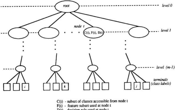
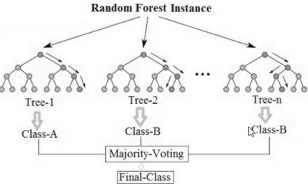
Experiment 2: Classification via Random Forest
Random forest or random decision forest (Ho, 1995) is an ensemble feature-based learning method for both classification and regression. RF is known to provide high accuracy even without fine tuning (Fernandez-Delgado et al., 2014), which makes it a popular ML algorithm. The basic building blocks of a random forest are decision trees