Advanced methods for prototype-based classification

(1)

Advanced methods for prototype-based classification

Schneider, Petra

IMPORTANT NOTE: You are advised to consult the publisher's version (publisher's PDF) if you wish to cite from it. Please check the document version below.

Document Version

Publisher's PDF, also known as Version of record

Publication date: 2010

Link to publication in University of Groningen/UMCG research database

Citation for published version (APA):

Schneider, P. (2010). Advanced methods for prototype-based classification Groningen: s.n.

Copyright

Other than for strictly personal use, it is not permitted to download or to forward/distribute the text or part of it without the consent of the author(s) and/or copyright holder(s), unless the work is under an open content license (like Creative Commons).

Take-down policy

If you believe that this document breaches copyright please contact us providing details, and we will remove access to the work immediately and investigate your claim.

Downloaded from the University of Groningen/UMCG research database (Pure): http://www.rug.nl/research/portal. For technical reasons the number of authors shown on this cover page is limited to 10 maximum.

(2)

Advanced methods for

prototype-based classification

(3)

problem; the alternative classification criteria are discussed in this thesis

ISBN: 978-90-367-4405-8

Published byAtto Producties Europe-Groningen www.attoproducties.nl

(4)

RIJKSUNIVERSITEIT GRONINGEN

Advanced methods for

prototype-based classification

Proefschrift

ter verkrijging van het doctoraat in de

Wiskunde en Natuurwetenschappen

aan de Rijksuniversiteit Groningen

op gezag van de

Rector Magnificus, dr. F. Zwarts,

in het openbaar te verdedigen op

maandag 14 juni 2010

om 14.45 uur

door

Petra Schneider

geboren op 19 mei 1980

te Darmstadt, Duitsland

(5)

Prof. dr. N. Petkov Beoordelingscommissie: Prof. dr. E. Mer´enyi

Prof. dr. T. Martinetz Prof. dr. M. Verleysen

(6)

Acknowledgments

Numerous people supported me in different ways to complete this thesis. Fore-most, very special words of thanks go to my promoter Prof. Michael Biehl. I highly appreciate that he gave me the opportunity to come to Groningen to work on this interesting and challenging project. His abilities as a highly qualified teacher and supervisor have accompanied and encouraged me throughout the years. Michael was always available for discussions and advice. He provided detailed feedback and critical comments on my work and I am grateful for this careful supervision.

In the same spirit, I like to thank my second promoter Prof. Nicolai Petkov for the valuable support and guidance in pursuing research. As the head of the Intelligent Systems group, Nicolai generated a friendly working environment. Furthermore, he provided financial support for conferences and workshops which gave me the opportunity to present my work to the machine learning community.

I deeply acknowledge the collaboration with Prof. Barbara Hammer. The inter-actions with her extensively inspired me. I am grateful that I could benefit from her knowledge and experience. Similarly, I am thankful to the other co-authors of my publications Prof. Thomas Villmann and Dr. Frank-Michael Schleif for the fruitful cooperation. I especially want to thank Barbara and Thomas another time for my research visits in Clausthal and Leipzig.

Although we did not work on common projects, I thank Dr. Michael Wilkinson for the informal help including LA_{TEX problems and other scientific issues. Lunch}

breaks with Michael were always interesting and I admire his profound knowledge on a wide range of topics.

I also like to thank Dr. Diane Black for her very constructive class about scientific writing. Diane was very helpful. Even after the end of the course, I always received quick response to the numerous questions I sent by E-Mail.

(11)

to name Aree Witoelar and Kerstin Bunte, who were kind officemates. Thanks for the good company and sharing knowledge and ideas in hours of joint time. It was a pleasure to work with you. I also really enjoyed Aree’s improv comedy shows and the activities with Kerstin at the ACLO sports center. Moreover, I thank Anarta Ghosh, Georgios Ouzounis, Erik Urbach, Giuseppe Pápari, Easwar Subra-manian, Florence Tushabe, Koen de Raedt, André Offringa, Ioannis Giotis, George Azzopardi, Fred Kiwanuka, Ernest Mwebaze and Ando Emerencia for the pleasant working atmosphere and the number of other activities beside scientific work. I am especially indebted to André for writing the Dutch summary of my thesis.

I appreciate the assistance of the institute staff. The secretaries Esmee Elshof, Desiree Hansen, Ineke Schelhaas and Helga Steenhuis were always supportive. Ad-ministrative issues were done efficiently by Alphons Navest, Janieta de Jong, An-nette Korringa and Yvonne van der Weerd. I also like to thank Harm Paas, Jurjen Bokma and Peter Arendz for system administration.

Finally, I express my special thanks to my family for providing me with a loving home and supporting my educational career in all non-scientific ways.

Petra Schneider Groningen May 10, 2010

(12)

Chapter 1

Introduction

This thesis presents research on Learning Vector Quantization (LVQ) which is a pop-ular family of machine learning algorithms. Machine learning is a subdiscipline of computer science inspired by neuroscience. It is concerned with the design of al-gorithms to optimize adaptive models on the basis of example data. In a learning environment, a model solves a certain problem related to a given data set. The samples are presented to the system and the learning algorithm adapts the model parameters such that similar input is processed better in the future. Learning from data is necessary, e.g., if the process which generates the data is unknown. In con-sequence, it is not possible to directly implement a computer program to solve the problem at hand. The objective of the learning process can be multifaceted. Machine learning covers a huge set of algorithms, e.g. for clustering, density estimation or classification and regression. Supervised learning algorithms work on labeled data, i.e. a target value is assigned to each datum and the model realizes an input output relationship. On the other hand, in an unsupervised learning scenario, the desired system output is unknown. A common goal of unsupervised learning methods is the detection of hidden patterns and regularities in the data. A broad overview of different topics addressed in machine learning can be found in Bishop (1995, 2007); Duda et al. (2000).

LVQ aims at classification, hence, the adaptive model implements a function which assigns input data to discrete categories. The term Learning Vector Quanti-zation specifies a class of supervised learning algorithms to derive a set of proto-typical vectors for the different categories of a given data set. Prototypes are vec-tor locations in feature space which reflect the characteristic attributes of the data in their direct neighborhood. The prototypes serve as typical representatives and provide an approximation of the data distribution. Many supervised and unsuper-vised machine learning techniques share the common idea of representing data by means of prototypes. Prominent unsupervised prototype-based methods are the

(13)

Self-organizing Map (SOM, Kohonen, 1997) and the Neural Gas algorithm (Mar-tinetz and Schulten, 1991). LVQ operates on labeled data and the learning algo-rithms identify class-specific prototypes. The set of prototypes in combination with a distance metric parameterizes a nearest prototype classification (NPC), i.e. an un-known pattern is assigned to the class which is represented by the closest prototype with respect to the selected metric.

LVQ is appealing for numerous reasons which will be highlighted throughout this thesis. Although the basic approach was introduced more than 20 years ago, LVQ is still an active field of research.

1.1 Scope of this study

The objective of this thesis is twofold: a new approach for metric adaptation in LVQ is presented and modifications of one specific learning algorithm, namely Robust Soft LVQ, are introduced.

Metric adaptation is a powerful approach to improve the performance of LVQ algorithms. Since the classifier’s decision depends on distances between prototypes and feature vectors, the selected metric is a key issue with respect to the learning dy-namics and the classification accuracy after training. Metric adaptation techniques allow to learn discriminative distance measures form example data, i.e. problem specific metrics can be derived. We present a novel adaptive distance measure which extends previously proposed methods for metric learning in LVQ. We show practical applications and focus on theoretical aspects of the novel metric learning scheme.

The proposed modifications of the Robust Soft LVQ algorithm concern three as-pects: the treatment of the algorithm’s hyperparameter, the decision rule for classi-fication, and we present a generalization of the algorithm with respect to vectorial class labels of the input data.

1.2 Outline

Chapter 2 provides a short introduction to Learning Vector Quantization. Nearest prototype classification and the original LVQ training algorithm (LVQ1) are intro-duced in detail. Furthermore, a number of alternative LVQ algorithms are presented with special focus on the methods we will use in this work. The algorithms of inter-est are Generalized LVQ (GLVQ) and Robust Soft LVQ (RSLVQ). An introduction to metric learning in LVQ concludes this introductory chapter.

(14)

1.2. Outline 3 first, the new distance measure is introduced in general form. The innovation con-sists of the extension of the Euclidean metric by a full matrix of adaptive weight factors. We derive the learning rules for matrix learning in GLVQ and RSLVQ. Ap-plications of the algorithms to artificial data and benchmark real life data sets illus-trate matrix learning in practical situations.

Chapter 4 further extends the previously proposed metric adaptation approach. Learning algorithms for adaptive distance measures may be subject to oversimplify the metric. In the context of matrix learning, this issue is discussed in detail in chapter 5. Here, we present a regularization scheme to prevent matrix learning al-gorithms from eliminating too many directions and to derive full rank matrices. The applicability of this technique is demonstrated by means of experiments on artificial data and real life data sets.

In chapter 5, we investigate the convergence behaviour of matrix learning al-gorithms. In simplified model situations, stationarity conditions of the metric pa-rameters can be derived. We consider unrestricted matrix learning as introduced in chapter 3, as well as the regularized learning procedures presented in chapter 4. The findings are verified by a set of practicals.

Chapter 6 focuses on Robust Soft LVQ in particular. Several extensions and mod-ifications of the original version of the algorithm are introduced. We present the application of the novel methods to a number of artificial- and real world data sets. Finally, a brief summary of the presented research and an outline for future work are given in chapter 7.

(15)

(16)

Chapter 2

Learning Vector Quantization

Abstract

The present chapter provides the required background information on Learning Vector Quantization. In particular, we explain nearest prototype classification in detail and present a set of LVQ learning algorithms. Furthermore, the concept of parameterized distance measures is introduced which allows metric learning. Already existing metric adaptation techniques in LVQ are shortly presented.

2.1 Introduction

Learning Vector Quantization is a supervised classification scheme which was in-troduced by Kohonen in 1986 (Kohonen, 1986). The approach still enjoys great pop-ularity and numerous modifications of the original algorithm have been proposed. The classifier is parameterized in terms of a set of labeled prototypes which repre-sent the classes in the input space in combination with a distance measured(·,·). To label an unknown sample, the classifier performs a nearest prototype classifica-tion, i.e. the pattern is assigned to the class represented by the closest prototype with respect tod(·,·). Nearest prototype classification is closely related to the popu-lark-nearest neighbor classifier (k-NN, Cover and Hart, 1967), but avoids the huge storage needs and computational effort ofk-NN. LVQ is appealing for several rea-sons: The classifiers are sparse and define a clustering of the data distribution by means of the prototypes. Multi-class problems can be treated by LVQ without mod-ifying the learning algorithm or the decision rule. Similarly, missing values do not need to be replaced, but can simply be ignored for the comparison between proto-types and input data; given a training pattern with missing features, the prototype update only affects the known dimensions. Furthermore, unlike other neural clas-sification schemes like the support vector machine or feed-forward networks, LVQ classifiers do not suffer from a black box character, but are intuitive. The prototypes reflect the characteristic class-specific attributes of the input samples. Hence, the models provide further insight into the nature of the data. The interpretability of

(17)

the resulting model makes LVQ especially attractive for complex real life applica-tions, e.g. in bioinformatics, image analysis, or satellite remote sensing (Biehl et al., 2006; Biehl, Breitling and Li, 2007; Hammer et al., 2004; Mendenhall and Mer´enyi, 2006). A collection of successful applications can also be found inBibliography on the Self-Organizing Map (SOM) and Learning Vector Quantization (LVQ)(2002).

The first LVQ algorithm (LVQ1) to learn a set of prototypes from training data is based on heuristics and implements Hebbian learning steps. Kohonen addition-ally proposed optimized learning-rate LVQ (OLVQ1) and LVQ2.1, two alternative (heuristic) training schemes which aim at improving the algorithm with respect to faster convergence and better approximation of Bayesian decision boundaries. LVQ variants which are derived from an explicit cost function are especially attractive al-ternatives to the heuristic update schemes. Proposals for cost functions to train LVQ networks were introduced in Sato and Yamada (1996); Seo and Obermayer (2003); Seo et al. (2003). The extension of cost function based methods with respect to a larger number of adaptive parameters is especially easy to implement. Furthermore, mathematical analysis of these algorithms can be investigated based on the respec-tive cost function (Sato and Yamada, 1998). In Crammer et al. (2003), it has been shown that LVQ aims at margin optimization, i.e. good generalization ability can be expected. A theoretical analysis of different LVQ algorithms in simplified model situations can also be found in Ghosh et al. (2006) and Biehl, Ghosh and Hammer (2007).

In distance-based classification schemes like Learning Vector Quantization, spe-cial attention needs to be paid to the employed distance measure. The Euclidean distance is a popular choice. Alternatively, quantities from information theory were used in Mwebaze et al. (2010). A huge set of LVQ variants aim at optimizing the distance measure for a specific application by means of metric learning (Bojer et al., 2001; Hammer and Villmann, 2002; Schneider et al., 2009a,b). Metric learning showed positive impact on the stability of the learning algorithms and the classification accu-racy after training. Furthermore, the interpretability of the resulting model increases due to the additional parameters. Metric adaption will also be a major subject of this thesis.

Moreover, researchers proposed the combination of LVQ with other prototype-based learning schemes like SOM or Neural Gas to include neighborhood cooper-ation into the learning process (Kohonen, 1998; Hammer, Strickert and Villmann, 2005b). Also, numerous techniques to realize fuzzy classification based on the gen-eral LVQ approach were proposed the last years (see, e.g. Thiel et al., 2008; Wu and Yang, 2003; Kusumoputro and Budiarto, 1999).

(18)

2.2. Nearest prototype classification 7

2.2 Nearest prototype classification

Let X ⊂ Rn _{be the input data space. Furthermore, the set} _{_y₁_{, ..., y}_C_} _specifies

the predefined target values of the classifier, i.e. the classes or categories. In this framework, objects are represented byn-dimensional feature vectors and need to be discriminated intoC different categories. Throughout this thesis, we always refer to the set of indices{1, ..., C}to depict class memberships.

A nearest prototype classifier is parameterized by a set of labeled prototype vec-tors and a distance metricd(·,·). The prototypes are defined in the same space as the input data. They approximate the samples belonging to the different categories and carry the label of the class they represent. At least one prototype per class needs to be defined. This implies the following definition

W₌_{₍_w_j_{, c}₍_w_j₎₎_|Rn_{× {}₁_{, . . . , C}_}}l_j₌₁_, _(2.1)

wherel≥C.W_{is also called the codebook.}

The classifier’s decision to label an unknown patternξis based on the distances of the input sample to the different prototypes with respect tod(·,·). NPC performs a winner-takes-all decision, i.e.ξis assigned to the class which is represented by the closest prototype

ξ_←c(wi), withwi= arg min

j d(wj,ξ), (2.2)

breaking ties arbitrarily. The setW_{in combination with the distance measure}

in-duces a partitioning of the input space (see Fig. 2.1). Each prototypewi has a so-called receptive fieldRiwhich is the subset of input space, wherewiis closer to the data than any other prototype. Formally,Riis defined by

Ri={ξ∈ X |d(ξ,wi)< d(ξ,wj),∀j 6=i}. (2.3) The prototypewi indicates the center of the receptive field. The distance measure

d(·,·) determines the shape of the decision boundaries. A popular metric is the Euclidean distance which is a special case of the general Minkowski distance

dp(w,ξ) = n X i=1 |ξi−wi|p !1/p , (2.4)

withp= 2. The Euclidean distance induces piecewise linear decision boundaries. More general decision boundaries can be realized by different valuesp(see Fig. 2.1) or local metrics which are defined for every class or every prototype individually.

The number of prototypes is a hyperparameter of the model. It has to be opti-mized by means of a validation procedure. Too few prototypes may not capture the

(19)

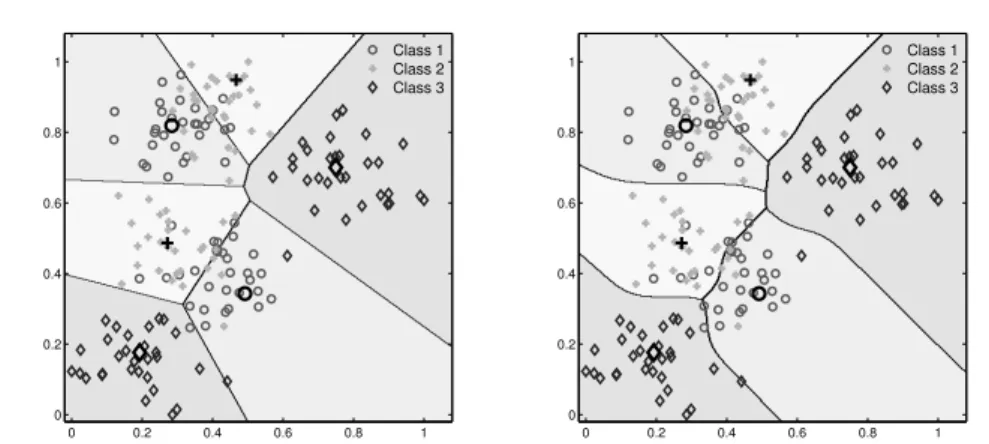
0 0.2 0.4 0.6 0.8 1 0 0.2 0.4 0.6 0.8 1 Class 1_{Class 2} Class 3 0 0.2 0.4 0.6 0.8 1 0 0.2 0.4 0.6 0.8 1 Class 1_{Class 2} Class 3

Figure 2.1:Visualization of the receptive fields of two nearest prototype classifiers. The data set realizes a three class problem. Each class is represented by two prototypes. The classifiers differ with respect to the employed distance measure. Left: Minkowski metric of orderp= 2. Right: Minkowski metric of orderp= 5.

structure of the data sufficiently. Too many prototypes cause over-fitting and induce poor generalization ability of the classifier.

2.3 Learning algorithms

LVQ algorithms are used to select the set of labeled prototypesW _{(see Eq. (2.1))}

which parameterizes an NPC. The learning process is based on a set of example dataX ₌_{₍_ξ

i, yi)|Rn× {1, . . . , C}}Pi=1called the training set. The objective of the

learning procedure is to place the prototypes in feature space in such a way that highest classification accuracy on novel data after training is achieved. In this work, we only consider so-called on-line learning algorithms, i.e. the elements of X_are

presented iteratively, and in each time stepµ, the parameter update only depends on the current training sample(ξ_µ, yµ). Depending on the learning algorithm,(ξµ, yµ) causes an update of one or severalwj. Prototypes, which are going to be updated, are moved in the direction ofξµ, if their class labels coincide withyµ. Otherwise, the prototypes are repelled. The general form of an LVQ update step can be stated as wj,µ=wj,µ−1+ ∆wj,µ =wj,µ−1+ α n f {wj,µ−1},ξµ, yµ (ξµ−wj,µ−1), (2.5)

withj = 1, . . . , l. The functionf specifies the algorithm. The parameterαis called

(20)

2.3. Learning algorithms 9 to be optimized by means of a validation procedure. It can be kept constant, or it can be annealed in the course of training based on a certain schedule. Furthermore, a favorable strategy to choose the initial prototype locations needs to be selected in advance, since the model initialization highly influences the learning dynamics and the success of training. In most applications, the mean value of the training sam-ples belonging to one class gives a good indication. Learning is continued until the prototypes converge, or until every element ofX_{was presented a certain number of}

times. One complete sweep through the training set is also called learning epoch. The first LVQ algorithm (LVQ1) was introduced by Kohonen. It performs Heb-bian learning steps and will be presented in Sec. 2.3.1. The methods extended in Chap. 3 are Generalized LVQ and Robust Soft LVQ. The algorithms are derived from explicit cost functions which will be introduced in Sec.s 2.3.2 and 2.3.3. Fur-ther LVQ variants will shortly be presented in Sec. 2.3.4.

2.3.1 LVQ1

In Kohonen’s first version of Learning Vector Quantization (Kohonen, 1986), the pre-sentation of a training sample causes an update of one prototype. In each iteration of the learning process, the prototype with minimal distance to the training pattern is adapted. Depending on the classification result, the winning prototype will be attracted by the training sample, or it will be repelled. Specifically, a learning step yields the following procedure:

1. Randomly select a training sample (ξ, y)

2. Determine the winning prototypewLwithd(wL,ξ) = minl{d(wl,ξ)}, breaking ties arbitrarily

3. UpdatewLaccording to

wL←wL+α·(ξ−wL), if c(wL) =y,

wL←wL−α·(ξ−wL), if c(wL)6=y.

(2.6)

Should the same feature vector be observed again,wL will give rise to a decreased (increased) distance, if the labelsc(wL)andyagree (disagree).

2.3.2 Generalized LVQ

GLVQ was introduced in Sato and Yamada (1996). The algorithm constitutes an LVQ variant which is derived from an explicit cost function. The GLVQ cost function is

(21)

heuristically motivated. However, as pointed out in Hammer, Strickert and Vill-mann (2005a), GLVQ training optimizes the classifier’s hypothesis margin. Hence, good generalization ability of GLVQ can be expected.

LetwJandwKbe the closest prototypes of training sample (ξ, y)withc(wJ) =y andc(wK)6=y. The GLVQ cost function is defined by

EGLVQ= P X i=1 Φ(µi), with µi= dJ(ξi)−dK(ξi) dJ(ξi) +dK(ξi) , (2.7)

wheredJ(ξ) = d(wJ,ξ)anddK(ξ) = d(wK,ξ)constitute the distances of pattern

ξto the respective closest correct and incorrect prototype. The termµis called the relative difference distance. It can be interpreted as a measure of confidence for prototype-based classification. The numerator is smaller than0iff the classification of the data point is correct. The smaller the numerator, the larger the difference of the distance from the closest correct and wrong prototype, i.e. the greater the security of the classifier’s decision. The denominator scales the argument ofΦsuch that it satisfies−1< µi<1. GLVQ aims at minimizingµifor all training samples in order to reduce the number of misclassifications. The scaling functionΦdetermines the active region of the algorithm.Φis a monotonically increasing function, e.g. the logistic functionΦ(x) = 1/(1 + exp(x))or the identityΦ(x) = x. For sigmoidal functions, the classifier only learns from training samples lying close to the decision boundary which carry most information. Training constitutes the minimization of

EGLVQ with respect to the model parameters. Sato and Yamada define the GLVQ

algorithm in terms of a stochastic gradient descent. The derivation of the learning rules can be found in Sato and Yamada (1996). A learning mechanism similar to the heuristic LVQ2.1 (see Sec. 2.3.4) results: the closest correct prototype is attracted by the current training sample, while the closest incorrect prototype is repelled. GLVQ training ensures convergence as pointed out in Sato and Yamada (1998).

2.3.3 Robust Soft LVQ

An alternative cost function was proposed by Seo and Obermayer in Seo and Ober-mayer (2003). The cost function of Robust Soft LVQ is based on a statistical modeling of the data, i.e. the probability density of the underlying distribution is described by a mixture model. Every componentjof the mixture is assumed to generate data which belongs to only one of theCclasses. The probability density of the full data set is given by a linear combination of the local densities

p(ξ_|W_{) =} C X i=1 l X j:c(wj)=i p(ξ_|j)P(j), (2.8)

(22)

2.3. Learning algorithms 11 where the conditional densityp(ξ|j)is a function of prototypewj. The densities can be chosen to have the normalized exponential form

p(ξ|j) =K(j)·expf(ξ,wj, σ2j), (2.9)

andP(j)is the prior probability that data are generated by mixture componentj. The class-specific density of classiconstitutes

p(ξ, i|W_{) =}

l

X

j:c(wj)=i

p(ξ|j)P(j). (2.10)

RSLVQ aims at maximization of the likelihood ratio of the class-specific distribu-tions and the unlabeled data distribution for all training samples

L= P Y i=1 p(ξi, yi|W) p(ξ_i_|W₎ . (2.11)

The algorithm’s cost function is defined by the logarithm ofL, hence

ERSLVQ= P X i=1 log p(ξi, yi|W) p(ξ_i|W₎ . (2.12)

RSLVQ training of the model parameters implements update steps in the direction of the positive gradient ofERSLVQ, see Seo and Obermayer (2003) for the derivation

of learning rules. Since the cost function is defined in terms of allwj, the complete set of prototypes is updated in each learning step. Correct prototypes are attracted by the current training sample, while incorrect prototypes are repelled. Note that the ratio in Eq. (2.11) is bounded by0≤ p_p(ξ₍_ξ,y_|W|W)) ≤1. Consequently, convergence of

the training procedure is assured.

Special attention needs to be paid to the parameterσ2_{. The variance of the}

Gaus-sians is an additional hyperparameter of the algorithm. It has crucial influence on the learning dynamics, since it determines the area in input space where training samples contribute to the learning process (see Seo and Obermayer, 2003, 2006, and Chap. 6 for details). The parameter needs to be optimized, e.g. by means of a validation procedure. Alternatively, the methods presented in Seo and Obermayer (2006) and Sec. 6.2.1 can be applied to cope with this issue. In the limit of vanish-ing softnessσ2 _→₀_{, the RSLVQ learning rule reduces to an intuitive crisp learning}

from mistakes (LFM) scheme: in case of erroneous classification, the closest correct and the closest wrong prototype are adapted along the direction pointing to / from the considered data point. Thus, a learning scheme very similar to LVQ2.1 (see Sec.

(23)

2.3.4) results which reduces adaptation to wrongly classified inputs close to the de-cision boundary. While the soft version as introduced in Seo and Obermayer (2003) leads to a good classification accuracy, the limit rule has some principled deficien-cies as shown in Biehl, Ghosh and Hammer (2007).

2.3.4 Further methods

This section roughly presents a set of other LVQ variants; please see the cited refer-ences for closer information. Note that this list is not complete. It presents just a few examples.

• OLVQ1(optimized-learning-rateLVQ1): The algorithm extends LVQ1 with

re-spect to individual, variable learning rates for all prototypes. Every prototype update according to Eq. (2.6) succeeds the modification of the accompanied learning rate. The parameter decreases in case of a correct classification and increases otherwise (see Kohonen, 1997, for the exact schedule).

• LVQ2.1: This modification of basic LVQ aims at a more efficient separation

of prototypes representing different classes. Given training sample(ξ, y)the two closest prototypeswi,wj are adapted, ifc(wi) =6 c(wj)andc(wi) = y. Additionally, the training sample needs to fall into the window defined by

min d(ξ,wi) d(ξ,wj), d(ξ,wi) d(ξ,wj) > s, with s= 1−ω 1 +ω. (2.13)

The hyperparameterω determines the width of the window, hence, it deter-mines the algorithm’s active region (see Kohonen, 1990, for details). The pro-totype update follows:

wi ←wi+α·(ξ−wi),

wj ←wj−α·(ξ−wj).

(2.14) The idea behind this heuristic training schemes is to shift the midplane of the two prototypes towards the Bayesian border. The window rule needs to be introduced to ensure convergence. Divergence turns out to be a problem es-pecially in case of unbalanced data sets.

• LVQ3: The algorithm is identical to the LVQ2.1, but provides an additional

learning rule if the two closest prototypes belong to the same class:

wi,j←wi,j+ε·α·(ξ−wi,j), (2.15)

with0 < ε < 1. The parameterεshould reflect the width of the adjustment

(24)

2.4. Adaptive distance measures in LVQ 13

2.4 Adaptive distance measures in LVQ

The methods presented in the previous section use the Euclidean distance (see Eq. (2.4)) to evaluate the similarity between prototypes and feature vectors. The Eu-clidean distance weights all input dimensions equally, i.e. equidistant points to a prototype lie on a hypersphere. This may be inappropriate, if the features are not equally scaled or are correlated. Furthermore, noisy dimensions may disrupt the classification, since they do not provide discriminative power, but contribute equally to the computation of distance values.

Metric adaptation techniques allow to learn discriminative distance measures from the training data, i.e. the distance measure can be optimized for a specific ap-plication. Metric learning is realized by means of a parameterized distance measure

dλ₍_·_,_·₎_{. The metric parameters}_λ_{are adapted to the data in the training phase. The} first approach to extend LVQ with respect to an adaptive distance measure is pre-sented in Bojer et al. (2001). The authors extend the squared Euclidean distance by a vectorλ∈Rn_{, λ}i_>₀_,P

iλi = 1of adaptive weight values for the different input dimensions: dλ(w,ξ) = n X i=1 λi(ξi−wi)2. (2.16)

The weightsλieffect a scaling of the data along the coordinate axis. The method pre-sented in Bojer et al. (2001) combines LVQ1 training (see Sec. 2.3.1) with Hebbian learning steps to updateλ. The algorithm is called Relevance LVQ (RLVQ). After training, the elementsλi reflect the importance of the different features for classi-fication: the weights of non-informative or noisy dimensions are reduced, while discriminative features gain high weight values;λis also called relevance vector.

The update rules for the metric parameters are especially easy to derive, pro-vided the LVQ scheme follows a cost function and the kernel is differentiable. How-ever, although this idea equips LVQ schemes with a larger capacity, the kernel has to be fixed a priori. The extension of Generalized LVQ (see Sec. 2.3.2) with respect to the distance measure in Eq. (2.16) was introduced in Hammer and Villmann (2002); the algorithm is called Generalized Relevance LVQ (GRLVQ).

Note that the relevance factors, i.e. the choice of the metric need not be global, but can be attached to single prototypes, locally. In this case, individual updates take place for the relevance factorsλjfor each prototype, and the distance of a data pointξfrom prototypewjis computed based onλj

dλj₍_ξ_,_w j) = n X i=1 λi j(ξi−wij). (2.17)

(25)

This allows local relevance adaptation, taking into account that the relevance might change within the data space. This method has been investigated e.g. in Hammer, Schleif and Villmann (2005).

Relevance learning extends LVQ in two aspects: It is an efficient approach to increase the classification performance significantly. At the same time, it improves the interpretability of the resulting model, since the relevance profile can directly be interpreted as the contribution of the dimensions to the classification. This specific choice of the similarity measure as a simple weighted diagonal metric with adap-tive relevance terms has turned out particularly suitable in many practical applica-tions, since it can account for irrelevant or inadequately scaled dimensions (see e.g. Mendenhall and Mer´enyi, 2006; Biehl, Breitling and Li, 2007; Kietzmann et al., 2008). For an adaptive diagonal metric, dimensionality independent large margin general-ization bounds can be derived (Hammer, Strickert and Villmann, 2005a). This fact is remarkable since it accompanies the good experimental classification results for high dimensional data by a theoretical counterpart. It has been shown recently that general metric learning based on large margin principles can greatly improve the results obtained by distance-based schemes such as thek-nearest neighbor classifier (Shalev-Schwartz et al., 2004; Weinberger et al., 2006).

(26)

Material based on:

Petra Schneider, Michael Biehl and Barbara Hammer -“Distance Learning in Discriminative Vector Quantization,”Neural Computation, vol. 21, no. 10, 2009.

Petra Schneider, Michael Biehl and Barbara Hammer -“Adaptive Relevance Matrices in Learning Vector Quantization,”Neural Computation, vol. 21, no. 12, 2009.

Chapter 3

Matrix learning in LVQ

Abstract

Learning vector quantization and extensions thereof offer efficient and intuitive classi-fiers which are based on the representation of classes by prototypes. The original meth-ods, however, rely on the Euclidean distance corresponding to the assumption that the data can be represented by isotropic clusters. For this reason, extensions of the methods to more general metric structures have been proposed such as relevance adaptation in generalized LVQ (GLVQ) and robust soft LVQ (RSLVQ). In these approaches, metric parameters are learned based on the given classification task such that a data driven dis-tance measure is found. We consider full matrix adaptation in advanced LVQ schemes; in particular, we introduce matrix learning to a recent statistical formalization of LVQ, robust soft LVQ, and we compare the results on several artificial and real life data sets to matrix learning in GLVQ, which is a derivation of LVQ-like learning based on a (heuris-tic) cost function. In all cases, matrix adaptation allows a significant improvement of the classification accuracy. Interestingly, however, the principled behavior of the mod-els with respect to prototype locations and extracted matrix dimensions shows several characteristic differences depending on the data sets.

3.1 Introduction

Discriminative vector quantization schemes such as learning vector quantization (LVQ) are very popular classification methods due to their intuitivity and robust-ness: they represent the classification by (usually few) prototypes which constitute typical representatives of the respective classes and, thus, allow a direct inspection of the given classifier. All the methods presented in Sec. 2.3, however, suffer from the problem that classification is based on a predefined metric. The use of Euclidean distance, for instance, corresponds to the implicit assumption of isotropic clusters.

(27)

Such models can only be successful if the data displays a Euclidean characteristic. This is particularly problematic for high-dimensional data where noise accumulates and disrupts the classification, or heterogeneous data sets where different scaling and correlations of the dimensions can be observed. Thus, a more general metric structure would be beneficial in such cases. The field of metric adaptation consti-tutes a very active research topic in various distance based approaches such as un-supervised or semi-un-supervised clustering and visualization (Arnonkijpanich et al., 2008; Kaski, 2001),k-nearest neighbor approaches (Strickert et al., 2007; Weinberger et al., 2006) and learning vector quantization (Hammer and Villmann, 2002; Schnei-der et al., 2009a). We will focus on matrix learning in LVQ schemes which accounts for pairwise correlations of features, i.e. a very general and flexible set of classifiers. On the one hand, we will investigate the behavior of generalized matrix LVQ (GM-LVQ) in detail, a matrix adaptation scheme for GLVQ which is based on a heuristic, though intuitive cost function. On the other hand, we will develop matrix adapta-tion for RSLVQ, a statistical model for LVQ schemes, and thus we will arrive at a uniform statistical formulation for prototype and metric adaptation in discrimina-tive prototype-based classifiers. We will introduce variants which adapt the matrix parameters globally based on the training set or locally for every given prototype or mixture component, respectively.

Matrix learning in GLVQ and RSLVQ will be evaluated and compared in dif-ferent learning scenarios: first, we consider test scenarios where prior knowledge about the form of the data is available. Furthermore, we compare the methods on two benchmarks from the UCI repository (Newman et al., 1998).

Interestingly, depending on the data, the methods show different characteris-tic behavior with respect to prototype locations and learned metrics. Although the classification accuracy is in many cases comparable, they display quite different be-havior concerning their robustness with respect to parameter choices and the char-acteristics of the solutions. We will point out that these findings have consequences on the interpretability of the results. In all cases, however, matrix adaptation leads to an improvement of the classification accuracy, despite a largely increased number of free parameters.

3.2 Advanced distance measure

We introduce an important extension of the concepts presented in Sec. 2.4, which employs a full matrix of adaptive relevances in the similarity measure. We consider a generalized distance of the form

(28)

3.2. Advanced distance measure 17 whereΛis a fulln×nmatrix which can account for correlations between the fea-tures. ForΛto define a valid metric, symmetry and positive definiteness has to be enforced (we will discuss in a moment how this property can be guaranteed). This way, arbitrary Euclidean metrics can be realized by an appropriate choice of the pa-rameters. In particular, correlations of dimensions and rotation of the axes can be accounted for. Such choices have already successfully been introduced in unsuper-vised clustering methods such as fuzzy clustering (Gath and Geva, 1989; Gustafson and Kessel, 1979), however, at the expense of increased computational costs, since these methods require a matrix inversion at each adaptation step. For the metric as introduced above, a variant which costsO(n2)can be derived.

Note that, as already stated, the above similarity measure defines a general squared Euclidean distance in an appropriately transformed space only ifΛis positive defi-nite and symmetric. We can achieve this by substituting

Λ = Ω⊤Ω (3.2)

which yieldsu⊤_Λ_u ₌ _u⊤_Ω⊤_Ω_u _{= Ω}⊤_u2 _≥ ₀_{for all}_u_{, where}_Ω_{is an arbitrary} realm×nmatrix, withm≤n. In this chapter, we focus on the special casem=n. In addition,det Λ 6= 0has to be enforced to guarantee thatΛis positive definite. However, in practice, positive semi-definiteness of the matrix is sufficient, since data often only populates a sub-manifold of the full data space and definiteness has to hold only with regard to the relevant subspace of data. Therefore, we do not enforce

det Λ6= 0. Using the relation in Eq. (3.2), the squared distance reads

dΛ(ξ,w) =X

ijk

(ξi−wi)ΩkiΩkj(ξj−wj).

Ωcan also be chosen to be symmetric, i.e.Ω⊤_{= Ω}_{. In this case, the distance measure} reads

dΛ(ξ,w) =X

ijk

(ξi−wi)ΩikΩkj(ξj−wj),

but we consider the more general case of non-symmetricΩthroughout the thesis. Note thatΩrealizes a linear transformation to anm-dimensional feature space. The metricdΛ_{corresponds to the squared Euclidean distance in this new coordinate}

system. This can be seen by rewriting Eq. (3.1) as follows:

dΛ(w,ξ) =(ξ−w)⊤Ω⊤ Ω(ξ−w)=Ω(ξ−w)2.

Hence, using the novel distance measure, the LVQ classifier is not restricted to the original features any more to classify the data. The system is able to detect alterna-tive directions in feature space which provide more discriminaalterna-tive power to sepa-rate the classes. Choosingm < nimplies that the classifier is restricted to a reduced

(29)

number of features compared to the original input dimensionality of the data. Con-sequently, rank(Λ) ≤ mand at leastn−meigenvalues ofΛare equal to zero. In many applications, the intrinsic dimensionality of the data is smaller than the orig-inal number of features. Hence, this approach does not necessarily constrict the performance of the classifier extensively.

Since the optimal matricesΛandΩare not known in advance, they have to be learned from example data during training. To obtain the adaptation formulas for the different learning algorithms, we need to compute the derivatives with respect tow andΩ. The derivatives ofdΛ₍_·_,_·₎_{with respect to}_w_{and a single element}_Ω

lm yield ∂dΛ₍_ξ_,_w₎ ∂w =−2 Ω ⊤_{Ω (} ξ−w) =−2 Λ (ξ−w), (3.3) ∂dΛ₍_ξ_,_w₎ ∂Ωlm = 2X i (ξi−wi)Ωli(ξm−wm). (3.4)

After every learning step,Λneeds to be normalized to prevent the learning algo-rithm from degeneration. One possibility is to enforce

X

i

Λii = 1, (3.5)

by dividing all elements ofΛby therawvalue ofP_iΛiiafter each step. In this way we fix the sum of diagonal elements which coincides with the sum of eigenvalues. This generalizes the normalization of relevancesPiλi = 1for a simple diagonal metric. One can interpret the eigendirections ofΛas the temporary coordinate sys-tem with the relevances corresponding to the eigenvalues. Since

Λii= X k ΩkiΩki = X k (Ωki)2, (3.6)

normalization can be done after every update step by dividing all elements ofΩby

(P_ki(Ωki)2)1/2= Pi[Ω⊤Ω]ii

1/2

.

We can work with one full matrix which accounts for a transformation of the whole input space, or, alternatively, with local matrices attached to the individual prototypes. In the latter case, the squared distance of data pointξfrom a prototype

wjis computed as

dΛj(wj,ξ) = (ξ−wj)⊤Λj(ξ−wj). (3.7) Each matrix is adapted individually. Localized matrices have the potential to take into account correlations which can vary between different classes or regions in fea-ture space. For instance, clusters with ellipsoidal shape and different orientation

(30)

3.3. Learning algorithms 19 could be present in the data. Note that local matrices imply nonlinear decision boundaries which are composed of quadratic pieces, unlike a global matrix which is characterized by piecewise linear decision boundaries. This way, the receptive fields of the prototypes need no longer be convex or even connected, as we will see in the experiments. Depending on the data at hand, this effect can largely increase the capacity of the system.

3.3 Learning algorithms

In the following, we derive the update rules for matrix learning in LVQ1, General-ized LVQ and Robust Soft LVQ.

3.3.1 Matrix LVQ1

Matrix LVQ1 (MLVQ1) is the heuristic extension of LVQ1 as described in Sec. 2.3.1. The algorithm realizes Hebbian updates for the closest prototypewLand the metric parameters. Accordingly, a learning step in MLVQ1 succeeds the following proce-dure:

1. Randomly select a training sample (ξ, y)

2. Determine the winning prototypewLwithdΛ(wL,ξ) = minl{dΛ(wl,ξ)}, breaking ties arbitrarily

3. UpdatewLaccording to wL←wL+α1·Λ·(ξ−wL), if c(wL) =y, wL←wL−α1·Λ·(ξ−wL), if c(wL)6=y (3.8) 4. UpdateΩaccording to Ω←Ω−α2·Ω·(ξ−wL)(ξ−wL)⊤, if c(wL) =y, Ω←Ω +α2·Ω·(ξ−wL)(ξ−wL)⊤, if c(wL)6=y, (3.9)

followed by a normalization step, andα2is the learning rate for the metric

param-eters. The matrixΛ = Ω⊤_Ω_{is updated in such a way that the distance}_dΛ₍_ξ_,_w L)is decreased in case of a correct classification, whiledΛ₍_ξ_,_w

L)increases, if the sample

(31)

3.3.2 Generalized Matrix LVQ

To extend GLVQ with respect to the generalized distance measure, we replace the squared Euclidean distance in Eq. (2.7) by the novel metric introduced in Eq. (3.1). The newly derived cost function will be calledEGMLVQ:

EGMLVQ= P X i=1 Φ(µΛi), with µΛi = dΛ J(ξi)−dΛK(ξi) dΛ J(ξi) +dΛK(ξi) , (3.10) wheredΛ

J(ξ) = dΛ(wJ,ξ)and dΛK(ξ) = dΛ(wK,ξ)constitute the distances of pat-tern(ξ, y)to the respective closest correct and wrong prototype. The derivatives of

EGMLVQwith respect towJandwKandΩlm(see Sec. 3.A.1) and the derivatives in Eq.s (3.3) and (3.4) yield the updates for the prototypes and the metric parameters

∆wJ = +α1·Φ′(µΛ(ξ))·µΛJ(ξ)·Λ·(ξ−wJ), (3.11) ∆wK =−α1·Φ′(µΛ(ξ))·µΛK(ξ)·Λ·(ξ−wK), (3.12) ∆Ωlm=−α2·Φ′(µΛ(ξ))· µΛJ(ξ)· (ξm−wJ,m) [Ω(ξ−wJ)]l − µΛK(ξ)· (ξm−wK,m) [Ω(ξ−wK)]l ! , (3.13) whereµΛ J(ξ) = 4dΛK(ξ)/(dΛJ(ξ) +dΛK(ξ))2 andµΛK(ξ) = 4dΛJ(ξ)/(dΛJ(ξ) +dΛK(ξ))2. Note that these updates correspond to the standard Hebb terms, pushing the closest correct prototype towards the considered data point and the closest wrong prototype away from the considered data point. The same holds for the update of the metric parameters, since the driving force consists of the derivative of the dis-tance from the closest correct prototype (scaled with−1) and the closest incorrect prototype. Thus, the parameters of the matrix are changed in such a way that the distance from the closest correct prototype becomes smaller, whereas the distance from the closest wrong prototype is increased. We name the algorithm defined by Eq.s (3.11) - (3.13) Generalized Matrix LVQ (GMLVQ).

In the experimental section, we also derive local relevance matrices attached to each prototype. Each matrix is adapted individually in the following way: given

(32)

up-3.3. Learning algorithms 21 dates yield ∆ΩJ,lm =−α2·Φ′(µΛ(ξ))· µΛJ(ξ)· (ξm−wJ,m)[ΩJ(ξ−wJ)]l , ∆ΩK,lm = +α2·Φ′(µΛ(ξ))· µΛK(ξ)· (ξm−wK,m)[ΩK(ξ−wK)]l . (3.14)

Consequently, the update rules for the prototypes (Eq.s (3.11),(3.12)) also contain the local matricesΛJ,ΛK. We refer to this generalized version of GMLVQ as localized GMLVQ (LGMLVQ).

3.3.3 Matrix Robust Soft LVQ

To extend RSLVQ by the more general metricdΛ₍_·_,_·₎_{, the conditional density}

func-tionp(ξ_|j)in Eq. (2.10) needs to be defined in terms of

f(ξ,w, σ2,Ω) = −(ξ−w) ⊤_Ω⊤_Ω(_ξ₋_w₎ 2σ2 , (3.15) with ∂f(ξ,w, σ2_,_Ω) ∂w = 1 σ2Ω ⊤_{Ω (}_ξ₋_w_{) =} 1 σ2Λ (ξ−w), (3.16) ∂f(ξ,w, σ2_,_Ω) ∂Ωlm =−_σ12 X i (ξi−wi) Ωli(ξm−wm) ! . (3.17)

Substitutingf(ξ,w, σ2_,_Ω)_{in Eq. (2.12) yields the cost function of the novel}

algo-rithm Matrix Robust Soft LVQ (MRSLVQ). The cost function is maximized by means of a stochastic gradient ascent. The derivative ofEMRSLVQwith respect to the model

parameters is stated in the appendix (see Sec. 3.A.2). Eq. (3.27) in combination with Eq.s (3.16) and (3.17) yields the update rules for the prototypes and the metric pa-rameters ∆wj= α1 σ2 (Py(j|ξ)−P(j|ξ))·Λ·(ξ−wj), c(wj) =y, −P(j|ξ)·Λ·(ξ₋wj), c(wj)6=y, (3.18)

(33)

∆Ωlm=− α2 σ2 · X j δy,c(wj)(Py(j|ξ)−P(j|ξ))−(1−δy,c(wj))P(j|ξ) · [Ω(ξ−wj)]l(ξm−wj,m) ! . (3.19)

The assignment probabilitiesPy(j|ξ)andP(j|ξ)are defined in Eq.s (3.30) and (3.31). Similar to local matrix learning in GMLVQ, it is also possible to train an individ-ual matrixΛj for every prototype. With individual matrices attached to all proto-types, the modification of Eq. (3.18) which includes the local matricesΛjis accom-panied by ∆Ωj,lm=−α2 σ2· " δy,c(wj)(Py(j|ξ)−P(j|ξ))−(1−δy,c(wj))P(j|ξ) · [Ωj(ξ−wj)]l(ξm−wj,m) # , (3.20)

under the constraintK(j) = const.for allj. We term this learning rule localized MRSLVQ (LMRSLVQ). Due to the restriction to constant normalization factorsK(j), the normalizationdet(Λj) =const.is assumed for this algorithm.

In the following experiments, we determine the algorithm’s hyperparpameter

σ2_{by means of a validation procedure. Alternatively, the parameter can be learned}

from the data which will be introduced in Sec. 6.2.

3.4 Experiments

With respect to parameter initialization and learning rate annealing, we use the same procedures in all experiments. The mean values of random subsets of training samples selected from each class are chosen as initial states of the prototypes. The learning rates are continuously reduced in the course of learning. Following Darken et al. (1992), we implement a schedule of the form

αi(t) =

αi

1 +τ(t−1) (3.21)

(i ∈ {1,2}), wheret counts the number training epochs. The factorτ determines the speed of annealing and is chosen individually for every application. The hy-perparameterσ2_{is held constant in all experiments with RSLVQ and MRSLVQ. To}

(34)

3.4. Experiments 23 normalize the relevance matrices after each learning step, we chooseP_iΛii= 1and initially setΛ =1_/n_{. Note that, in consequence, the Euclidean distance in RSLVQ}

and GLVQ has to be normalized to one as well to allow for a fair comparison with respect to learning rates. Accordingly, the RSLVQ- and GLVQ prototype updates and the functionfin Eq. (2.9) have to be weighted by1/n.

3.4.1 Artificial data

In the first experiments, the algorithms are applied to the artificial data from Bojer et al. (2001) to illustrate the training of an LVQ-classifier based on the alternative cost functions with fixed and adaptive distance measure. The data sets 1 and 2 comprise three-class classification problems in a two dimensional space. Each class is split into two clusters with small or large overlap, respectively (see Fig. 3.1). We randomly select 2/3 of the data samples of each class for training and use the remaining data for testing. According to the a priori known distributions, the data is represented by two prototypes per class. We use the learning parameter settings

G(M)LVQ:4α1= 0.005, 4α2= 0.001

(M)RSLVQ: α1= 5·10−4, α2= 1·10−4

τ = 0.001and perform 1000 sweeps through the training set. The results presented in the following are averaged over 10 independent constellations of training and test set. We apply several different valuesσ2_{from the interval [0.001, 0.015] and present}

the simulations giving rise to the best mean performance on the training sets. The results are summarized in Tab. 3.1. They are obtained with the hyperpa-rametersσ2

opt(RSLVQ) = 0.002andσ2opt(MRSLVQ) = 0.002,0.003for data set 1 and 2, respectively. The use of the advanced distance measure yields only a slight im-provement compared to the fixed Euclidean distance, since the distributions do not

Table 3.1: Mean rate of misclassification (in %) obtained by the different algorithms on the artificial data sets 1 and 2 at the end of training. The values in brackets are the variances.

Data set 1 Data set 2

Algorithm εtrain εtest εtrain εtest

GLVQ 2.0 (0.02) 2.7 (0.07) 19.2 (0.9) 24.2 (1.9) GMLVQ 2.0 (0.02) 2.7 (0.07) 18.6 (0.7) 23.0 (1.6) RSLVQ 1.5 (0.01) 3.7 (0.04) 12.8 (0.07) 19.3 (0.3) MRSLVQ 1.5 (0.01) 3.7 (0.02) 12.3 (0.04) 19.3 (0.3)

(35)

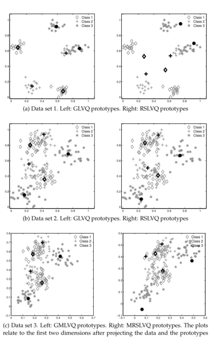
(a) Data set 1. Left: GLVQ prototypes. Right: RSLVQ prototypes

(b) Data set 2. Left: GLVQ prototypes. Right: RSLVQ prototypes

0 0.1 0.2 0.3 0.4 0.5 0.6 0.7 −0.1 0 0.1 0.2 0.3 0.4 0.5 0.6 0.7 0.8 Class 1 Class 2 Class 3 −0.1 0 0.1 0.2 0.3 0.4 0.5 0.6 −0.1 0 0.1 0.2 0.3 0.4 0.5 0.6 Class 1 Class 2 Class 3

(c) Data set 3. Left: GMLVQ prototypes. Right: MRSLVQ prototypes. The plots relate to the first two dimensions after projecting the data and the prototypes withΩGMLVQandΩMRSLVQ, respectively.

Figure 3.1: Artificial data. Prototype constellations identified by GLVQ, RSLVQ, GMLVQ and MRSLVQ in a single run on different data sets.

(36)

3.4. Experiments 25 0 0.2 0.4 0.6 0.8 1 0 0.2 0.4 0.6 0.8 1 0 0.1 0.2 0.3 0.4 0.5 0.6 0 0.2 0.4 0.6 0.8 1 0 0.2 0.4 0.6 0.8 1 0 0.1 0.2 0.3 0.4 0.5 0.6

(a) Data set 1. Left: Attractive forces. Right: Repulsive forces. The plots relate to the hyperparameterσ2= 0.002. 0 0.2 0.4 0.6 0.8 1 0 0.2 0.4 0.6 0.8 1 0 0.1 0.2 0.3 0.4 0.5 0.6 0.7 0 0.2 0.4 0.6 0.8 1 0 0.2 0.4 0.6 0.8 1 0 0.1 0.2 0.3 0.4 0.5 0.6 0.7

(b) Data set 2. Left: Attractive forces. Right: Repulsive forces. The plots relate to the hyperparameterσ2_{= 0}_.₀₀₂_.

Figure 3.2:Artificial data.Visualization of the update factors(Py(j|ξ)−P(j|ξ))(attractive forces) andP(j|ξ)(repulsive forces) of the nearest prototype with correct and incorrect class label on data sets 1 and 2.

have favorable directions to classify the data. On data set 1, GLVQ and RSLVQ show nearly the same performance. However, the prototype configurations identified by the two algorithms vary significantly (see Fig. 3.1a). During GLVQ-training, the prototypes move close to the cluster centers in only a few training epochs, resulting in an appropriate approximation of the data by the prototypes. On the contrary, pro-totypes are frequently located outside the clusters, if the classifier is trained with the RSLVQ-algorithm. This behavior is due to the fact that only data points lying close to the decision boundary change the prototype constellation in RSLVQ significantly (see Eq. (3.18)). As depicted in Fig. 3.2a, only a small number of training samples are lying in the active region of the prototypes while the great majority of training samples attains only tiny weight values which are not sufficent to adjust the pro-totypes to the data in reasonable training time. This effect does not have negative

(37)

impact on the classification of the data set. However, the prototypes do not provide a reasonable approximation of the data.

The prototype constellation identified by RSLVQ on data set 2 represents the classes clearly better (see Fig. 3.1b). Since the clusters show significant overlap, a sufficiently large number of training samples contributes to the learning process (see Fig. 3.2b) and the prototypes quickly adapt to the data. The good approximation of the data is accompanied by an improved classification performance compared to GLVQ. Although GLVQ also places prototypes close to the cluster centers, the use of the RSLVQ-cost function gives rise to the superior classifier for this data set. This observation is also confirmed by the experiments with GMLVQ and MRSLVQ.

To demonstrate the influence of metric learning, data set 3 is generated by em-bedding each sample ξ = (ξ1, ξ2) ∈ R2 of data set 2 in R10 by choosing: ξ3 =

ξ1+η1, . . . ξ6=ξ1+η4, whereηicomprises Gaussian noise with variances 0.05, 0.1,

0.2 and 0.5, respectively. The featuresξ7, . . . , ξ10contain pure uniformly distributed

noise in [-0.5, 0.5] and [-0.2, 0.2] and Gaussian noise with variances 0.5 and 0.2, re-spectively. Hence, the first two dimensions are most informative to classify this data set. The dimensions 3 to 6 still partially represent dimension 1 with increasing noise added. Finally, we apply a random linear transformation on the samples of data set 3 in order to construct a test scenario, where the discriminating structure is not in parallel to the original coordinate axis any more. We refer to this data as data set 4. To train the classifiers for the high-dimensional data sets we use the same learning parameter settings as in the previous experiments.

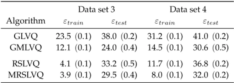
The obtained mean rates of misclassification are reported in Tab. 3.2. The results are achieved using the hyperparameter settingsσ2

opt(RSLVQ) = 0.002,0.003and

σ2

opt(MRSLVQ) = 0.003for data set 3 and 4, respectively. The performance of GLVQ

Table 3.2: Mean rate of misclassification (in %) obtained by the different algorithms on the artificial data sets 3 and 4 at the end of training. The values in brackets are the variances.

Data set 3 Data set 4

GLVQ 23.5 (0.1) 38.0 (0.2) 31.2 (0.1) 41.0 (0.2) GMLVQ 12.1 (0.1) 24.0 (0.4) 14.5 (0.1) 30.6 (0.5) RSLVQ 4.1 (0.1) 33.2 (0.5) 11.7 (0.1) 36.8 (0.2) MRSLVQ 3.9 (0.1) 29.5 (0.4) 8.0 (0.1) 32.0 (0.2)

(38)

3.4. Experiments 27 Off−diagonal elements 2 4 6 8 10 2 4 6 8 10 −0.1 −0.05 0 0.05 0.1 1 2 3 4 5 6 7 8 9 10 0 0.5 1 Diagonal elements 1 2 3 4 5 6 7 8 9 10 0 0.5 1 Eigenvalues Off−diagonal elements 2 4 6 8 10 2 4 6 8 10 −0.1 −0.05 0 0.05 0.1 1 2 3 4 5 6 7 8 910 0 0.5 1 Diagonal elements 1 2 3 4 5 6 7 8 910 0 0.5 1 Eigenvalues

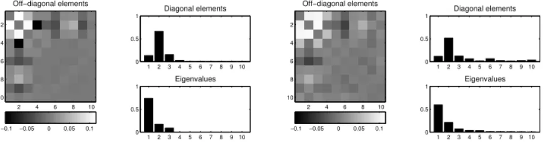
Figure 3.3: Artificial data. Visualization of the relevance matrices ΛGMLVQ (left) and ΛMRSLVQ(right) obtained in one training run on data set 3. The diagonal elements are set to zero in the visualization of the off-diagonal elements.

clearly degrades due to the additional noise in the data. However, by adapting the metric to the structure of the data, GMLVQ is able to achieve nearly the same accu-racy on data sets 2 and 3. A visualization of the resulting relevance matrixΛGMLVQ

is provided in Fig. 3.3, left. The diagonal elements turn out that the algorithm totally eliminates the noisy dimensions 4 to 10, which, in consequence, do not contribute to the computation of distances any more. As reflected by the off-diagonal elements, the classifier additionally takes correlations between the informative dimensions 1 to 3 into account to quantify the similarity of prototypes and feature vectors. In-terestingly, the algorithms based on the statistically motivated cost function show strong overfitting effects on this data set. Obviously, the number of training ex-amples in this application is not sufficient to allow for an unbiased estimation of the correlation matrices of the mixture model. MRSLVQ does not detect the rele-vant structure in the data sufficiently to reproduce the classification performance achieved on data set 2. The respective relevance matrix trained on data set 3 (see Fig. 3.3, right) depicts that the algorithm does not totally prune out the uninforma-tive dimensions. The superiority of GMLVQ in this application is also reflected by the final position of the prototypes in feature space (see Fig. 3.1c). A comparable result for GMLVQ can even be observed after training the algorithm on data set 4. Hence, the method succeeds to detect the discriminative structure in the data, even after rotating or scaling the data arbitrarily.

3.4.2 Real life data

Beyond, we apply the algorithms to two benchmark data sets provided by the UCI repository of Machine Learning (Newman et al., 1998), namely Image Segmentation and Letter Recognition.

(39)

Image segmentation data set

The data set contains 19-dimensional feature vectors, which encode different at-tributes of 3×3 pixel regions extracted from outdoor images. Each such region is as-signed to one of seven classes (brickface, sky, foliage, cement, window, path, grass). The features 3-5 are (nearly) constant and are eliminated for these experiments. As a further preprocessing step, the features are normalized to zero mean and unit vari-ance. The training set contains 210 data points (30 samples per class), the test data consists of 300 samples per class. We split the test data into a test and a validation set of equal size in order to optimize the model settings.

Each class is approximated by one prototype, respectively. We use the parame-ters settings

G(M)LVQ:4α1= 0.005, 4α2= 0.0001

(M)RSLVQ: α1= 0.0001, α2= 0.0001,σ2= 0.04

τ = 0.0001and continue learning until the validation error remains constant or starts indicating overfitting effects. In order to reduce the influence of random fluc-tuations, we average our results over ten runs with varying initializations.

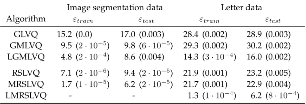
The obtained classification accuracies are summarized in Table 3.3. For both cost function schemes, the performance improves significantly by adapting the dis-tance measure. Remarkably, RSLVQ and MRSLVQ clearly outperform the respective GLVQ methods on this data set.

Comparing the resulting relevance matrices in Fig. 3.4 shows that GMLVQ and

Table 3.3: Mean rate of misclassification (in %) obtained by the different algorithms on the image segmentation and letter data set at the end of training. The values in brackets constitute the variances.

Image segmentation data Letter data

GLVQ 15.2 (0.0) 17.0 (0.003) 28.4 (0.002) 28.9 (0.003) GMLVQ 9.5 (2·10−5₎ _{9.8 (}₆_·₁₀−5₎ _{29.3 (0.002)} _{30.2 (0.002)} LGMLVQ 4.8 (2·10−4₎ _{8.6 (0.004)} _{14.3 (}₃_·₁₀−4₎ _{16.0 (0.002)} RSLVQ 7.1 (2·10−6₎ _{9.4 (}₂_·₁₀−5₎ _{21.9 (0.001)} _{23.2 (0.005)} MRSLVQ 1.7 (1·10−5₎ _{6.2 (}₂_·₁₀−5₎ _{21.7 (0.001)} _{22.9 (0.004)} LMRSLVQ - - 1.3 (1·10−4) 6.2 (8·10−4)

(40)

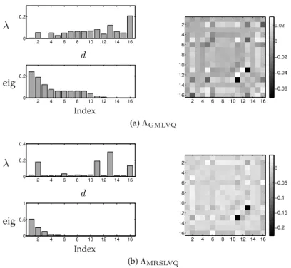
3.4. Experiments 29 λ eig Index 2 4 6 8 10 12 14 16 0 0.2 2 4 6 8 10 12 14 16 0 0.2 d 2 4 6 8 10 12 14 16 2 4 6 8 10 12 14 16 −0.06 −0.04 −0.02 0 0.02 (a)ΛGMLVQ λ eig Index 2 4 6 8 10 12 14 16 0 0.2 0.4 2 4 6 8 10 12 14 16 0 0.5 1 d 2 4 6 8 10 12 14 16 2 4 6 8 10 12 14 16 −0.2 −0.15 −0.1 −0.05 0 (b)ΛMRSLVQ

Figure 3.4: Image segmentation data. Visualization of the relevance matrixΛafter 1500 epochs of GMLVQ-training and MRSLVQ-training.Left:Diagonal elements and eigenvalues.

Right:Off-diagonal elements. The diagonal elements are set to zero for the plot.

MRSLVQ identify the same dimensions as being most discriminative to classify the data. The features which achieve the highest weight values on the diagonal are the same in both cases. But note that the feature selection by MRSLVQ is clearly more pronounced. The eigenvalue profiles reflect that MRSLVQ uses a smaller number of features to classify the data. It is visible that especially relations between the di-mensions encoding color information are emphasized. The didi-mensions weighted as most important are features 11: exred-mean (2R - (G + B)) and 13: exgreen-mean (2G - (R + B)) in both classes. Furthermore, the off-diagonal elements highlight correlations with e.g. feature 8: rawred-mean (average over the regions red val-ues), feature 9: rawblue-mean (average over the regions green valval-ues), feature 10: rawgreen-mean (average over the regions green values). For a description of the features, see Newman et al. (1998).

Based onΛGMLVQ, distances between prototypes and feature vectors obtain much

smaller values compared to the MRSLVQ-matrix. This is depicted in Fig. 3.7a which visualizes the distributions of the distancesdΛ

(41)

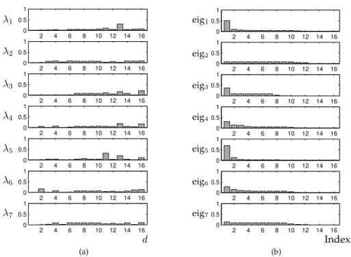
in-λ1 λ2 λ3 λ4 λ5 λ6 λ7 2 4 6 8 10 12 14 16 0 0.5 1 2 4 6 8 10 12 14 16 0 0.5 1 2 4 6 8 10 12 14 16 0 0.5 1 2 4 6 8 10 12 14 16 0 0.5 1 2 4 6 8 10 12 14 16 0 0.5 1 2 4 6 8 10 12 14 16 0 0.5 1 2 4 6 8 10 12 14 16 0 0.5 1 d (a) eig1 eig2 eig3 eig4 eig5 eig6 eig7 2 4 6 8 10 12 14 16 0 0.5 1 2 4 6 8 10 12 14 16 0 0.5 1 2 4 6 8 10 12 14 16 0 0.5 1 2 4 6 8 10 12 14 16 0 0.5 1 2 4 6 8 10 12 14 16 0 0.5 1 2 4 6 8 10 12 14 16 0 0.5 1 2 4 6 8 10 12 14 16 0 0.5 1 Index (b)

Figure 3.5:Image segmentation data.(a) Diagonal elements of local relevance matricesΛ1−7. (b) Eigenvalue spectra of local relevance matricesΛ1−7.

correct prototype. 90% of all test samples attain distancesdΛ

J <0.2by the GMLVQ classifiers. This holds for only 40% of the feature vectors, if the MRSLVQ classifiers are applied to the data. This observation is also reflected by the distribution of the data and the prototypes in the transformed feature spaces (see Fig. 3.8a). After pro-jection withΩGMLVQthe data comprises very compact clusters with high density,

while the samples and prototypes spread wider in the coordinate system detected by MRSLVQ.

In a further sequence of GMLVQ experiments, we analyse the algorithm’s sen-sitivity with respect to the number of prototypes. We determine the class-wise rates of misclassification after each experiment and repeat the training providing one fur-ther prototype for the class contributing most to the overall rate of misclassification. A system consisting of 10 prototypes achieves 90.9% mean test accuracy, using 13 prototypes reaches 91.2% mean accuracy on the test sets. The slight improvement in classification performance is accompanied by an increasing training time until con-vergence.

(42)

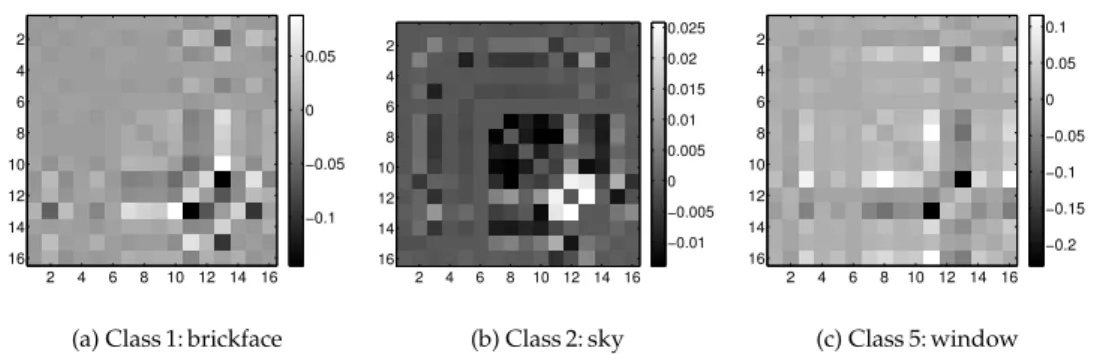
3.4. Experiments 31 2 4 6 8 10 12 14 16 2 4 6 8 10 12 14 16 −0.1 −0.05 0 0.05

(a) Class 1: brickface

2 4 6 8 10 12 14 16 2 4 6 8 10 12 14 16 −0.01 −0.005 0 0.005 0.01 0.015 0.02 0.025 (b) Class 2: sky 2 4 6 8 10 12 14 16 2 4 6 8 10 12 14 16 −0.2 −0.15 −0.1 −0.05 0 0.05 0.1 (c) Class 5: window Figure 3.6:Image segmentation data.Visualization of the off-diagonal elements of the local matricesΛ1,2,5. The diagonal elements are set to zero for the plot.

previous GMLVQ experiments. The training error remains constant after approx-imately 12 000 sweeps through the training set. The validation error shows slight over-fitting effects. It reaches a minimum after approximately 10 000 epochs and increases in the further course of training. In the following, we present the results obtained after 10 000 epochs. At this point, training of individual matrices per pro-totype achieves a test accuracy of 94.4%. We are aware of only one SVM result in the literature which is applicable for comparing the performance. Prudent and Ennaji (2005) achieve 93.95% accuracy on the test set.

Figure 3.5 shows the diagonal elements and eigenvalue spectra of all local ma-trices we obtain in one run which are also representative for the other experiments. Matrices with a clear preference for certain dimensions on the diagonal also display a distinct eigenvalue profile (e.g. Λ1,Λ5). Similarly, matrices with almost balanced

relevance values on the diagonal exhibit only a weak decay from the first to the sec-ond eigenvalue (e.g. Λ2,Λ7). This observation for diagonal elements and

eigenval-ues coincides with a similar one for the off-diagonal elements. Figure 3.6 visualizes the off-diagonal elements of the local matricesΛ1,Λ2andΛ5. Corresponding to the

balanced relevance- and eigenvalue profile of matrixΛ2, the off-diagonal elements

are only slightly different from zero. This may indicate diffuse data without a pro-nounced, hidden structure. There are obviously no other directions in feature space which could be used to significantly minimize distances within this class. On the contrary, the matricesΛ1andΛ5show a clearer structure. The off-diagonal elements

cover a much wider range and there is a clearer emphasis on particular dimensions. This implies that class-specific correlations between certain features have significant influence. The most distinct weights for correlations with other dimensions are ob-tained for features, which also gain high relevance values on the diagonal.

Advanced methods for prototype-based classification

Advanced methods for prototype-based classification

Schneider, Petra

Advanced methods for

prototype-based classification

RIJKSUNIVERSITEIT GRONINGEN

Advanced methods for

prototype-based classification

Proefschrift

ter verkrijging van het doctoraat in de

Wiskunde en Natuurwetenschappen

aan de Rijksuniversiteit Groningen

op gezag van de

Rector Magnificus, dr. F. Zwarts,

in het openbaar te verdedigen op

maandag 14 juni 2010

om 14.45 uur

door

Petra Schneider

geboren op 19 mei 1980

te Darmstadt, Duitsland

Contents

Acknowledgments

Chapter 1

Introduction

1.1

Scope of this study

1.2

Outline

Chapter 2

Learning Vector Quantization

2.1

Introduction

2.2

Nearest prototype classification

2.3

Learning algorithms

2.3.1

LVQ1

2.3.2

Generalized LVQ

2.3.3

Robust Soft LVQ

2.3.4

Further methods

2.4

Adaptive distance measures in LVQ

Chapter 3

Matrix learning in LVQ

3.1

Introduction

3.2

Advanced distance measure

3.3

Learning algorithms

3.3.1

Matrix LVQ1

3.3.2

Generalized Matrix LVQ

3.3.3

Matrix Robust Soft LVQ

3.4

Experiments

3.4.1

Artificial data

3.4.2

Real life data