Sánchez Lozano, Enrique (2017) Continuous
regression: a functional regression approach to facial
landmark tracking. PhD thesis, University of Nottingham.
Access from the University of Nottingham repository:
http://eprints.nottingham.ac.uk/43300/1/ESL_Thesis_ID4235858_June2017.pdf Copyright and reuse:
The Nottingham ePrints service makes this work by researchers of the University of Nottingham available open access under the following conditions.
This article is made available under the University of Nottingham End User licence and may be reused according to the conditions of the licence. For more details see:
http://eprints.nottingham.ac.uk/end_user_agreement.pdf
Computer Science
Computer Vision Laboratory
Continuous Regression
A Functional Regression approach to Real-time
Facial Landmark Tracking
Enrique S´
anchez-Lozano
Submitted in part fulfilment of the requirements for the degree of Doctor of Philosophy in Computer Science of the University of Nottingham,
Facial Landmark Tracking (Face Tracking) is a key step for many Face Analysis systems, such as Face Recognition, Facial Expression Recognition, or Age and Gender Recognition, among others. The goal of Facial Landmark Tracking is to locate a sparse set of points defining a facial shape in a video sequence. These typically include the mouth, the eyes, the contour, or the nose tip. The state of the art method for Face Tracking builds on Cascaded Regression, in which a set of linear regressors are used in a cascaded fashion, each receiving as input the output of the previous one, subsequently reducing the error with respect to the target locations. Despite its impressive results, Cascaded Regression suffers from several drawbacks, which are basically caused by the theoretical and practical implications of using Linear Regression. Under the context of Face Alignment, Linear Regression is used to predict shape displacements from image features through a linear mapping. This linear mapping is learnt through the typical least-squares problem, in which a set of random perturbations is given. This means that, each time a new regressor is to be trained, Cascaded Regression needs to generate perturbations and apply the sampling again. Moreover, existing solutions are not capable of incorporating incremental learning in real time. It is well-known that person-specific models perform better than generic ones, and thus the possibility of personalising generic models whilst tracking is ongoing is a desired property, yet to be addressed.
This thesis proposes Continuous Regression, a Functional Regression solution to the least-squares problem, resulting in the first real-time incremental face tracker. Briefly speaking, Continuous Regression approximates the samples by an estimation based on a first-order Taylor expansion yielding a closed-form solution for theinfinite set of shape displacements. This way, it is possible to model the space of shape displacements as a continuum, without the need of using complex bases. Further, this thesis introduces a novel measure that allows Continuous Regression to be extended to spaces of correlated variables. This novel solution is incorporated into the Cascaded Regression framework, and its computational benefits for training under different configurations are shown. Then, it presents an approach for incremental learning within Cascaded Regression, and shows its complexity allows for real-time implementation. To the best of my knowledge, this is the first incremental face tracker that is shown to operate in real-time. The tracker is tested in an extensive benchmark, attaining state of the art results, thanks to the incremental learning capabilities.
I would like to start this by thanking my advisors Dr. Michel Valstar and Dr. Yorgos Tz-imiropoulos. The final outcome of this thesis wouldn’t be possible without your help and support. Both of you have spent lots of time teaching me valuable things, about writing, about research, about the way things should be done... but not only this, you also spent a valuable amount of time in teaching me how to handle my feelings. Although this “lecture” is still underway, I think we have made some progress on this. Thanks for your support in the hardest parts of this period. It definitely made me not give up and complete this piece of work.
Thanks to Dr. Jos´e Luis Alba-Castro. You always have the time to chat and discuss about everything, and I have to recognise that you were like my second father at the School of Telecommunications (given that he was also there!), and somehow I have to be thankful for all your help. Also, my special thanks to Dr. Daniel Gonz´alez-Jim´enez, my first advisor, who always was the lucid person to say what was correct for all of us. I would like to also thank Dr. Fernando De la Torre, who lit my spark in theoretical research, with an application to real-life problems. Thanks for the opportunity you brought to me to have an amazing time at Carnegie Mellon, and live an unforgettable experience.
Thanks to all the Computer Vision Laboratory people. The Lab is probably one of the best environments I have found to work at. It is a pleasure to work with people who are driven by the aim to succeed in academic research, but collaborative and willing to help and spend their time helping other peers. Besides, I have to thank my colleagues for making the Lab a place in which one can balance work and life, so that one can succeed in both, and we can always enjoy a couple of pints and have fun when we feel stuck. It is impossible for me to name all of you, but I want to highlight those that stood my changeable mood day by day: the B86 Lab people: Aaron, Adrian, Dottie and Themos. This was a nice crew. Also, thanks to Brais, who was really helpful in key moments, I appreciate your help and advice. Thanks to Joy for her priceless support on language correctness. I cannot forget about Paula, who was a really good lab mate, and now is still a good friend.
Thanks to all those friends that were, are, and hope will be, there time to time to enjoy a beer. Patri, Jose, David, Ernesto, and all SM Color friends, who always bring me a warm welcome in the basketball court. Thanks to Miguel, it is always a pleasure to catch up with you.
A special thanks to my family: Pili, Quique, Marta, Alberto, Susa, Pilar and Manolo. Good and unforgettable times. There are no words to express my gratitude.
And finally, thanks to Marta Dominguez, who knows me and stays there day and night no matter what happens. Any word here would mean nothing compared to everything you gave to me all this time. This acknowledgment has to be extended to Lluvia and Nika as well. You will not read this, but you three are the most important thing that ever happened to me.
Ao meu pai, Dr. Enrique S´anchez S´anchez (8-Xullo-1955, 19-Decembro-2015).
Thanks for your time, all the things you taught me, and your eagerness to make me want to be a good person, no matter any academic title or position. I still feel I am learning from you.
A mi madre, Mar´ıa Del Pilar Lozano Escolar (30-Septiembre-1957).
Por tu santa paciencia.
‘T´uzaro!’ ESS
Abstract i Acknowledgements iii 1 Introduction 1 1.1 Contributions . . . 10 1.2 Outline . . . 11 1.3 Publications . . . 12 2 Background Theory 14 2.1 Problem definition . . . 14 2.2 Notation . . . 15 2.3 Shape Model . . . 16 2.4 Appearance Model . . . 20 2.5 Fitting approaches . . . 24 3 Literature Review 25 3.1 Literature Review in Face Alignment and Tracking . . . 25
3.1.1 Active Shape Models . . . 26 vii
viii CONTENTS
3.1.2 Active Appearance Models . . . 28
3.1.3 The Inverse Compositional framework . . . 31
3.1.4 Constrained Local Models . . . 34
3.1.5 Regression Methods . . . 39
3.1.6 Cascaded Regression . . . 43
3.1.7 Towards the first benchmark in face tracking . . . 54
3.1.8 Databases . . . 55
3.2 Review of Functional Regression . . . 57
3.2.1 Functional Regression in Computer Vision . . . 59
3.3 Challenges and Opportunities . . . 62
4 Continuous Regression 65 4.1 Introduction . . . 66
4.1.1 Contributions . . . 70
4.2 Linear Regression for Face Alignment . . . 70
4.2.1 Training . . . 71
4.3 Continuous Regression . . . 72
4.3.1 1-D Continuous Regression . . . 73
4.4 2n-dimensional Continuous Regression . . . 77
4.5 Complexity . . . 79
4.6 Experiments . . . 82
4.6.1 1d-Continuous Regression . . . 82
4.7 Conclusions . . . 87
5 Continuous Regression on Correlated Variables 90 5.1 Introduction . . . 92
5.2 A new measure for Functional Regression . . . 94
5.3 Cascaded Continuous Regression . . . 98
5.3.1 Complexity . . . 98
5.4 Functional Covariance for PCA in CCR . . . 99
5.5 Geometric interpretation . . . 101
5.6 Use of a PDM . . . 103
5.7 Experiments . . . 105
5.7.1 Equivalence with SDM . . . 105
5.7.2 The impact of the data term . . . 106
5.7.3 Use of a PDM . . . 107
6 Incremental Cascaded Continuous Regression 110 6.1 Introduction . . . 113
6.2 Incremental Cascaded Continuous Regression . . . 116
6.3 Complexity . . . 118
6.4 Experimental results . . . 119
6.4.1 Experimental set-up . . . 120
6.4.2 Tracking System . . . 122
7 Conclusion 134
7.1 Applications . . . 135 7.2 Future Work . . . 136
Bibliography 139
6.1 AUC for 49 points configuration for the different categories. . . 125 6.2 AUC for 66 points configuration for the different categories (68 for Yang et al.
(2015), Xiao et al. (2015)). . . 125
1.1 Sample pictures taken fromhttp://www.crowdemotion.co.uk/(upper-left) and
http://www.releyeble.com/(upper-right). Both companies offer an automated analysis of users emotions, so that further marketing and advertising can be done upon potential interest. Thebottomimage shows the case studies offered by Vis-age Technologies. As can be seen, the applications range is huge. . . 3
1.2 The set of points belonging to a shape. As can be seen, these points are sorted so that each point will always index a specific key location . . . 5
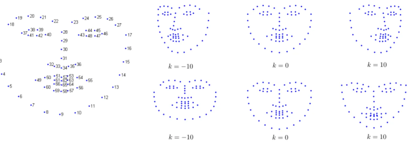
2.1 Fitting process for both detection (Top) and tracking (Bottom) tasks. The detection starts with roughly locating the face and initialising the points with the mean shape. Then, the fitting is done using a learnt model. Tracking differs from detection in the way the initialisation (and subsequently, the training) is done. Given the image at framet+ 1, the fitting starts with the points located at framet. . . 16 2.2 Left Shape example, labelled following a specific distribution. During training,
all faces are labelled following this distribution, so that the problem is consistent.
Right Rows correspond to the variation of the first two modes of the shape model, respectively. These faces were generated by setting the i-th element of
c to k, and the remaining parameters to zero. That is, s =s0 +kBis, where k
is the constant used to show the variation, and Bi
s is the i-th column (1 in the
upper row of the image, 2 in the lower row) of the shape basis. . . 20 xiii
xiv LIST OF FIGURES
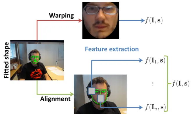
2.3 Different methods for extracting features from a facial image. Topimage depicts theholisticrepresentation of the face. The face is warped back from the original image to the mean shape, and then the whole convex hull defined by the external points defines the image within which features are extracted. Bottom image depicts the part-based feature extraction. First of all, the image is aligned so that scale, rotation and translation are removed, so that these artifacts do not affect the feature extraction process. Then, a patch around each point is defined, from which features are extracted, and further concatenated to form the final descriptor. . . 23
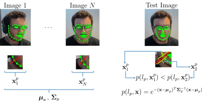
3.1 Left: The training of a patch expert for point p, done by collecting the pixels along the normal surface of target point (red line), and computing the average and covariance of the normals for the training set (µand Σ). Right: The local search consists of sampling along different candidates on the normal surface to find which candidate yields the minimum Mahalanobis distance. As we can see, the second candidate yields a higher probability of being correctly aligned, and thus we select its centre. . . 27
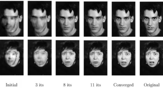
3.2 The process of fitting an AAM to an image. The shape is deformed so that an instance of the appearance model matches as much as possible to the input image. This image has been taken from Cootes et al. (2001) . . . 31
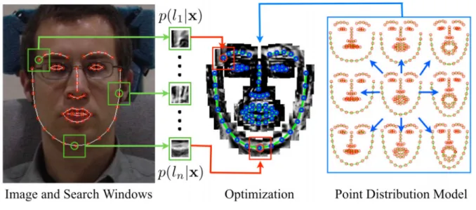
3.3 This image has been taken from Saragih et al. (2011), and illustrates the main CLMs steps. First of all, a local search returns the probability of each of the landmarks to be correctly aligned. Then, we have to find the PDM instance that best fits the located points. . . 36
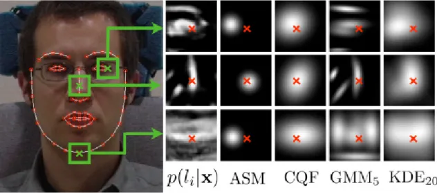
3.4 This image has been taken from Saragih et al. (2011), and illustrates the different ways of approximating the response maps. . . 39
3.5 Example illustrating the problem of variance in Linear Regression. Blue dots are training examples, and green lines correspond to displacements towards the ground-truth, depicted by the red line. In a convenient abuse of terminology, we see a linear regressor in this one dimensional example as the average training displacement. The orange dot is a test sample, for which a prediction is made, resulting in the orange arrow. In both cases the test sample is the same. However, in the first scenario, with lower training variance, the regressor is capable of accurately predict the displacement, while in the second scenario, the regressor is far from being optimal for the given test sample. . . 44
3.6 Weak invariant features. The yellow coordinates represent the rotation of the given image, and the red arrow represents the pose relative to the local coordi-nates (control points). The second image results after applying δθ to both the image and the control points, thus resulting in the same features. Thereby, we can say this kind of features to be weakly invariant. . . 45
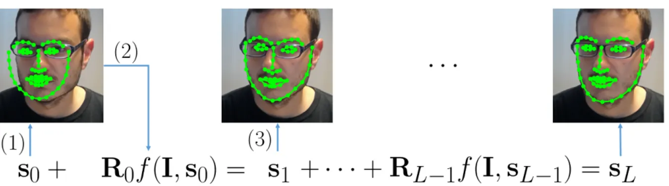
3.7 Cascaded regression fitting. First of all (1) we are given an initial shapes0 from
the face detection bounding box. Then, the first step consists of estimating s1
from the features extracted in s0 and the regressor R0 learnt for the initial step.
Then, this process is repeated for the set of L regressors learnt for the model. . . 50
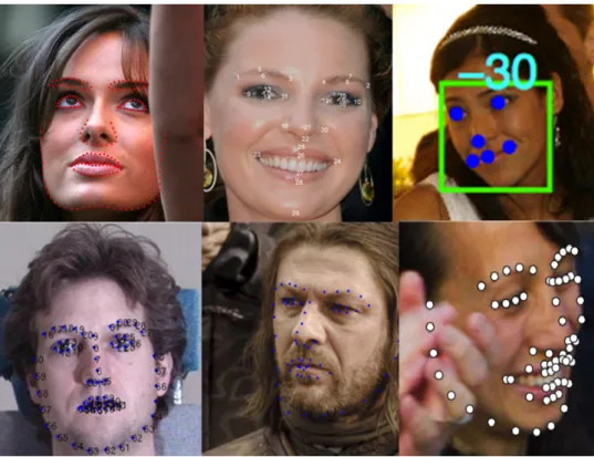
3.8 Images with annotations from different databases. From left to right, top to bottom: Helen, LFPW, AFW, Multi-PIE, Ibug, 300W. . . 57
4.1 Difference between sampling-based regression and continuous regression. In Con-tinuous Regression, we consider all the samples within a predefined neighbour-hood, whereas in sampling-based approaches we need to generate the data from a given distribution. . . 66
xvi LIST OF FIGURES
4.2 We can think of Continuous Regression in a different way. The green dot repre-sents the ground-truth position, black arrows represent the shape displacements, yellow crosses represent the perturbations. a) In sampling-based regression we generate a set of random perturbations and then we extract the features around the perturbed samples (black square around the yellow crosses). b) We can then replace the sampled features by a Taylor approximation; to do so we only need the ground-truth features (the green box surrounding the ground-truth position). The features at the yellow crosses are given by a Taylor approximation. c) The Taylor expansion linearises the features with respect to the shape displacements, and hence we can add as many samples as we want, being these approximated by the Taylor expansion given by the image features and Jacobians, extracted at the ground-truth positions. d) We can extend the number of samples to the infinite, covering all possible displacements within a neighbourhood of the ground-truth positions (black box). This implies that the sum over perturbations is replaced by an integral. In this Chapter we will see that there is a closed form solution to this problem. . . 67
4.3 Mean errors for the predictions given by discrete regressors (in red) and con-tinuous regressors (in green). Each plot shows a configuration in which the chosen limit is set to the value shown in the corresponding title (i.e., a = 1,2,5,10,20,50). Errors are measured in the same subset of images compos-ing the traincompos-ing set, the number of which is also varied in this experiment. It can be seen that the Continuous Regression gives a constant error no matter the number of training samples, given that it does not account for perturbations, but rather for image features. Also, it can be seen that, the bigger the input variance, the lower the capacity of Continuous Regression. In this setting, the discrete regressor needs 1000 perturbations to perform reasonable well. . . 84
4.4 Mean errors for the predictions given by Continuous Regression under different configurations. We can see that the best step is given by ∆x= 1, although for bigger limits this assumption stops being correct. However, the behaviour of Continuous Regression for such limits can not be associated to the chosen step, given that all configurations generally fail to recover from a huge initial error. . 85
4.5 Comparison between performance given by a regressor trained with HOG, and a regressor trained with Pixels. We can see that the pixels perform better than HOG only for very small perturbations given that the Taylor approximation is still valid. However, when considering further distances, we have to note that a “smoother” feature descriptor, such as HOG, attains better results than pixels. 86
4.6 Comparison of Continuous Regression and Sampling-based Linear Regression, in which both training and testing perturbations depend on the value of a. #tr
represents the number of training images. . . 88
4.7 Comparison of Continuous Regression and Sampling-based Linear Regression, in which both training and testing perturbations depend on the value of a. #tr
represents the number of training images. . . 89
5.1 Left: Average shapeµresulting after computing the shape displacements across the training set of videos. It can be seen that it is almost zero, thus we can assume that displacements are unbiased. Right: Covariance matrix Σ ∈ R132×132 of
the shape displacements measured across the set of training videos. As can be seen, the covariance matrix is far from being diagonal. Therefore, we cannot approximate the covariance matrix by its diagonal elements. . . 93
5.2 a) Functional Regression as explained in Chapter 4. b) The new approach to Continuous Regression, studied in this Chapter, can be seen as the inverse of a Monte Carlo sampling estimation. The probability density function defined by
p(δs) defines the geometric space within which samples are taken. . . 95 5.3 Differences between the classical Functional Regression formulation (Left) and
the CR in correlated variables (Right). The shadowed green area represents the volume within which samples are taken. Left image corresponds to a diagonal covariance matrix, with entries defined as a32. Right image corresponds to a full covariance matrix and a non-zero mean vector. The sampling space is moved to the centre of coordinates defined byµ, and rotated according to the eigenvectors of Σ. . . 102
xviii LIST OF FIGURES
5.4 Cumulative Error Distribution (CED) curve for both the CCR and SDM methods in the test partition of the 300VW. The Area Under the Curve for both methods
is the same. This illustrates that CCR and SDM are equivalent. . . 106
5.5 Cumulative Error Distribution (CED) curve for both the uncor-CR (green) and cor-CR (blue). Results are shown for the 49 points configuration. The contribu-tion of a full covariance matrix is clear . . . 107
5.6 Performance achieved by a model using a PDM, and a model not using it. The results show that both methods perform equally, and therefore the use of a PDM is beneficial, given its computational advantages. . . 108
5.7 Top: Mean shape parameters displacement across the training set of videos (µ). Bottom: Covariance matrix (Σ) of shape parameter displacements. For the sake of visualisation, left image shows the covariance of rigid parameters, and right image shows the covariance of non-rigid parameters. . . 109
5.8 Results comparing a model trained using full covariance matrices with a model trained using only diagonal covariance matrices. Both models use the same PDM. We can see that, given that the covariance matrix is not completely diagonal, the use of a full covariance matrix, and hence the approach presented in this Chapter, is still beneficial. . . 109
6.1 Cumulative curves for a generic model (red) trained using the LFPW training partition set, and using the first 100 frames of the specific video (blue). Left image shows the cumulative error for the whole video, and right image shows the cumulative error for frames 101 to end. . . 111
6.2 Overview of our incremental cascaded continuous regression algorithm (iCCR). The originally model RT learned offline is updated with each new frame, thus sequentially adapting to the target face. . . 113
6.3 CED’s for the 49-points configuration (category A). . . 126
6.4 CED’s for the 49-points configuration (category B). . . 127
6.7 CED’s for the 66-points configuration (category B). . . 130 6.8 CED’s for the 66-points configuration (category C). . . 131 6.9 Qualitative results for a sample video of Category 3. Top row shows the tracked
points using iCCR, whereas bottom row shows the results given by the CCR without incremental learning. The importance of incremental learning is there-fore clear. . . 132 6.10 Qualitative results for a sample video of Category 3. Top row shows the tracked
points using iCCR, whereas bottom row shows the results given by the CCR without incremental learning. The importance of incremental learning is there-fore clear. . . 133
Ea , a-dimensional Identity matrix
1a , a-dimensional vector with all elements set to 1
s , Shape
p , Shape parameters
s∗, p∗ , Ground-truth shape / shape parameters
s0 , Mean shape
x, x∗ , Image features / Features extracted at the ground-truth positions
f, f(s),f(p) , Image features extracting function
D , Dimensionality of the feature vector
d , Dimensionality of the feature vector after dimensionality reduction
f0 , Derivative of feature extraction function f
J,J∗ , Jacobian of image features / Jacobian of image features evaluated at the ground-truth positions
Ba , Matrix of appearance bases
Bs , Matrix of shape bases
N , Number of training images
K , Number of perturbations per image
µ , Mean vector of shape (parameters) displacements
Σ , Covariance matrix of shape (parameters) displacements
p(.) , Probability distribution (pdf)
M , [µ,Σ+µµT]
B , µ1 Σ+µµµT T
D∗i , [x∗i,J∗i] Ground-truth data for imagei
¯
Chapter 1
Introduction
Recent years have seen the field of Human-Computer Interaction, or HCI, growing fast, up to a level in which it is natural for us to interact with machines, even though the interaction itself may not yet be natural. The time where only experts were capable of using machines is over; now we are all1 surrounded by computers, and users are now in charge. It is thus a fact that we are embracing a great challenge in making machines easily accessible and handled by everyone. New methods other than the classical mouse and keyboard have been developed to improve our interaction with novel devices. For instance, fingertips emerged as the natural tool to interact with recent mobile devices, and keyboards are being used less. Nowadays, cameras are embedded in even unimaginably small devices, and mobile phones have become the new de-facto portable cameras, which are now easily accessible and low-priced. Among all new methods, or tools, to interact with machines, one that is attracting a lot of attention is the face.
Faces are a main signal for humans when interacting with others. Our faces reveal important information about us. They reveal who we are (identity), our age and gender (i.e., our demo-graphic group), and even our ethnicity. Faces also reveal our emotional state, such as whether we are angry, happy, disgusted, sad or surprised. It has been shown that facial expressions are universal with respect to emotional responses (Ekman & Oster 1979). Besides this, our
1Better said: we wish we were, though there is still a huge challenge in making machines, along with other
resources, accessible toall. See for example the problem of the “digital divide”.
face displays some of our social traits, such as our personality. We can generally tell whether a specific face belongs to an extrovert person, or whether it belongs to an easy-going person. Re-cently, new datasets and challenges have emerged aimed at using Computer Vision to effectively predict these traits (Ponce-Lopez et al. 2016). Finally, our faces reveal certain social signals (Pentland 2007), such as our willingness to buy a specific product, as well as our comfort when interacting with other people.
It is thus a research target to determine how humans behave by analysing their faces, and how faces can be modelled by means of analysing their spatio-temporal appearance variations. Even further, people demand easier ways to control devices: we want to unlock our mobile phones using our faces, or have a camera take a picture whenever we show a smile. All of these face-computer interactions are typically included in different mainstream research fields: face recognition, age and gender estimation, facial expression recognition and social traits. Face recognition, as well as age and gender estimation attempt to model identity, subject to appearance and aging factors, as well as age and gender themselves. On the other hand, facial expression recognition and social trait classification typically aims to analyse the spatio-temporal variation of faces, in terms of their expressions, and how we perceive and classify them. These topics are now of increasing demand in cross disciplinary research fields, such as entertainment, health, education or marketing. Typically, these cross disciplinary fields are also categorised within the novel field of “Affective Computing”, which gathers Computer Vision, Psychology, Medicine and Neuromarketing into a field of research that ultimately attempts to make machines interact with users in an affective way; that is to say, based upon their emotional responses.
Regarding entertainment applications using faces, we barely need words to describe the success of Apps such as Snapchat (https://www.snapchat.com/), or Masquerade (http: //msqrd.me/). In the field of marketing, we find many companies now dedicated to video an-alytics, such as Visage Technologies (https://visagetechnologies.com/), Releyeble (http: //www.releyeble.com/), or CrowdEmotion (http://www.crowdemotion.co.uk/). All these start-ups build mainly upon analysing users’ faces, to provide the customer with certain metrics that might be used to promote some products over others. These companies offer an enclosed
3
Figure 1.1: Sample pictures taken from http://www.crowdemotion.co.uk/ (upper-left) and
http://www.releyeble.com/ (upper-right). Both companies offer an automated analysis of users emotions, so that further marketing and advertising can be done upon potential interest. The bottom image shows the case studies offered by Visage Technologies. As can be seen, the applications range is huge.
product capable of giving the customer all the behaviour metrics taken from the users. This is becoming increasingly important, because it allows machines to analyse huge amounts of data automatically and almost in real time, thus helping retailers focus on maximising their benefits over the market space. A sample picture is shown in Figure 1.1, where the products are clearly focused on improving market success.
But, even though marketing and entertainment appear to be the most visible fields of applica-tion, we cannot leave aside health and education. The automated analysis of faces is helping
health in many ways. To name few: the automatic assessment of chronic pain (Aung et al. 2015, Egede et al. 2017), the detection of depression and concealing depression (Solomon et al. 2015), distinguishing between Autism Spectrum Disorder and Attention Deficit
Hyperactiv-ity Disorder (Jaiswal et al. 2017), estimating the gestational age of newborns (Torres Torres et al. 2017), or the automated support of children with autism syndrome with “affective” video games (Gordon et al. 2014). In general, one can discern a number of medical conditions that alter expressive behaviour. Such conditions have been coined ’Behaviomedical’ (Valstar 2014), with the science of monitoring or treating such conditions coined ’Behaviomedics’. Similarly,
education can benefit from newer advances in face analysis. The field of “Affective Tutoring Systems” (Ammar et al. 2010) has recently proven to improve how students engage in certain subjects they might feel are difficult, being driven by an automated system that can show content based on their emotional responses.
All of this illustrates the wide field of applications in which analysing faces plays an important role. But, what does “analysing faces” mean for a Computer Vision scientist? Certainly, it can be seen as a black box receiving an image or a video, and returning a class, where class can mean, e.g., whether a face is smiling or not, or whether it belongs to an specific person or not. The black box needs to process the image, by first locating the face and extracting some image descriptors, and then predicts the target class. In this whole process, the first step is crucial for the performance of any subsequent step. That is to say, precisely locating the face is very important. The more accurate the location of the face, the better the classification task will be, since any further analysis can be done in a more semantically meaningful way. For example, a small patch of pixels is more semantically meaningful if it is known that the appearance pertains to the mouth and is centred on a lip corner point, rather than being a specific block in a regular grid returned by a face detector. The simplest way of locating a face is by detecting a bounding box around the face; a problem that is known as “face detection”, which has been widely studied within the Computer Vision community. However, relying only on such a vague location will lead to extracting image information in a poor way. That is to say, one would better analyse the face once a semantic meaning has been assigned to each of its elements: if we know that a specific region of the face is a mouth, we can further process it given that contextual knowledge. For instance, let us assume that we want to detect when someone smiles, using the geometric deformation of the mouth. If we just detect the face and align it with respect to the bounding box, we might not know where the mouth is. Thus,
5
sometimes we will extract information from the moustache, the chin, or anywhere else but the mouth. Hence, localising the face more accurately would improve the performance of the smile detector.
Figure 1.2: The set of points be-longing to a shape. As can be seen, these points are sorted so that each point will always index a specific key location
The problem of locating a set of points within a face, such as the mouth, the eyes, or the contour, is known as Face Alignment, or Facial Point Localisation, when it refers to static images, and as Face Tracking when it refers to video sequences. Typically, Face Alignment starts from an average shape placed within the bounding box given by a face detector, whereas Face Tracking takes advantage of the fact that faces move smoothly (given a sufficiently high fram-erate), to start from the points estimated at the previous frame. Thus, despite being trained in a similar way, they differ in some important aspects. In any case, Face Tracking algorithms adapt existing techniques from Face Alignment
methods, and most of the methods to date exploit different techniques for Face Alignment, leav-ing aside the real-time capabilities that are crucial for a trackleav-ing system. The contributions of this thesis are thus in the field of Face Tracking: the system resulting from the application of the techniques presented herein is the first face tracking system capable of working in real-time whilst performing incremental learning. We will later see what incremental learning is and why it is so important. The set of points consisting of those target locations is known as shape. Figure 1.2 depicts what we refer to as a set of points, or shape. Thus, we can state that an accurate localisation of the points belonging to a shape is a key step for most face analysis systems. However, despite it being the first step (the second if we consider face detection as the first, separated from the face alignment step), for all the applications described above, it is still an open research topic in Computer Vision. The development of an accurate tracking or localisation system, with real-time capabilities, is still underway.
We can perhaps discern two breakthroughs in the field of Face Alignment. The first one can be traced back to the early 00’s, in which Cootes et al. (2001) proposed Active Appearance Models
(AAMs). AAMs are simply a statistical way to describe deformable objects (faces in our case), by allowing the points describing them (the shapes), and the corresponding appearances (the pixels), to vary under a small number of degrees of freedom, known as parameters. This way, AAMs provide a linear basis of an object’s representation, in which any object instance can be represented by a linear combination of the basis. These bases capture the way objects vary by means of both shape and appearance. In other words, AAMs represent faces by a small set of parameters, encoding how shapes and appearances vary. We can therefore generate as many instances of the models (i.e., faces) as we want, just by changing the values of this small set of parameters. The face alignment problem was presented in Cootes et al. (2001) as the problem of finding the parameters that best describe an input face. These parameters are found by minimising a reconstruction error, named residual, measuring how much an instance of the model looks like the target face. We can say that the AAMs sparked the field of Face Alignment; the work of Cootes et al. is among the most cited works within all disciplines of Computer Science (> 12000 citations in its 3 main papers Cootes et al. (1995, 1998, 2001)). We will briefly review the AAMs work in Chapter 3.
The AAMs influenced face alignment research in the past decade, especially after the land-mark paper of Matthews & Baker (2004), who revisited many features of the original paper, proposing novel optimisation procedures for them. More specifically, they proposed an Inverse Compositional Framework (IC), which became the state of the art until the end of the 00’s. However, despite the success of both AAMs and the IC, they were limited in some ways: they were hindered by a lack of generalisation, and, most importantly, were slow, and thus not suitable for a wide range of applications. The generalisation problem of AAMs and IC comes from the fact that they are generative: the localisation is based on the residual between the image and an instance of the model, meaning that, the less similar the face is with respect to the model, the harder it is for the model to fit it properly. For instance, a model generated from female faces will likely fail when fitting a male face. In that sense, the generalisation capabilities are said to be person-dependent.
Follow-up works attempted to overcome these two main limitations. Different methods were proposed: graphical models (Valstar et al. 2010), boosting (Liu 2011), and exhaustive
con-7
strained search (Saragih et al. 2011). These methods are typically classified as discriminative: they attempt to learn how to estimate the real locations (from here called the ground-truth locations), given the current information (i.e., the current shape estimate and the appearance). That is to say, they “discriminate”, i.e., differentiate, a good localisation from a wrong one, and thus look for the location that would have the highest discriminative score. A simple approach for discriminative methods is using a Linear Regressor (Tresadern et al. 2010). The use of Linear Regression is simple: if we have a set of annotated images (known as training set), we can systematically displace the ground-truth of each of them, and extract some local descriptors (known as features). The regressor will be a map from these descriptors towards the displacement that has been applied to the ground-truth for the features to be taken, i.e., a Linear Regressor extracts some local information from a current estimate of where the points are, and then predicts where these points should be moved to be closer to the ground truth. However, we can not include all possible displacements from any region of the image and as-sume a single regressor will accurately learn from all of them. It is known that, the bigger the input variance (i.e., the range of input shapes), the lower the capacity of a regressor to work well. There is a trade-off between robustness and sensitivity of a regressor. In order to bypass this trade-off, Cao et al. (2012) adapted the Cascaded Regression approach of Doll´ar et al. (2010), to the space of shapes. However, the most successful form of Cascaded Regression is the Supervised Descent Method (SDM) (Xiong & De la Torre 2013). Briefly speaking, the SDM consists of a set of linear regressors in cascade, in which each regressor utilises the output shape of the previous one to predict a new shape, in a coarse-to-fine strategy. If the fitting process will always start with an average shape, we can train a regressor tasked with only rigid variations of that shape. Then, the second regressor will take the expected output and predict a new shape, and so forth. This way, the first level of the cascade will be highly robust at the cost of not being very precise, whereas subsequent levels will become gradually more sensitive, at the cost of retaining robustness. This novel approach revolutionised the state of the art in the field, bringing to the fore a fast and accurate method for landmark localisation, also suitable for tracking tasks. As of 2016, the SDM is considered a state-of-the-art method for face alignment and tracking.
However, the cascaded regression algorithm still suffers from three major limitations. First of all, the training, which is formulated by means of the common Least Squares problem, needs an exponential number of samples with respect to the dimensionality of the image descriptors in order for the models not to be biased. In general, the number of perturbations per image is small, and thus these will be biased. When creating a small number of samples, these hardly meet the distribution that has generated them. Second, it is still an open question how the training data, as well as their corresponding initialisations, affect performance in a specific scenario. In addition, training a cascaded regression model is computationally expensive. The training process is slow and requires data to be collected (i.e., sampled) each time a new model is to be trained for a different configuration. This way, training different models under different configurations is not feasible in many cases. Moreover, the computational cost of training a model grows exponentially with the number of cascade levels, the number of images used, and the number of perturbations generated per image. Finally, and more importantly, state of the art methods in cascaded regression are not capable of updating trained models in real time. It is well known that person-specific models will perform better than generic methods when the target person is known(Gross et al. 2005). However, training a person dependent model for each potential user is impossible in practice. Thus, a method capable of updating a tracker’s model given the user’s information, and in real-time, is a desired property for generic models. As we shall see, state-of-the-art methods are far too slow to be updated online when the tracking is ongoing.
Building upon the Cascaded Regression framework, this thesis analyses the three problems above, and ultimately presents a novel approach for the Linear Regression training, with an application to face tracking. It is important to distinguish the tasks of localisation in still images (detection) and in videos (tracking), since the former has no prior information and has to detect the facial landmarks from a given face detection, whereas the latter exploits temporal information. While the detection problem has been widely tackled in the literature, little attention has been paid to the tracking stage. There are two main reasons behind this: the first one is that existing methods were typically too slow, and thus impractical for the task of real-time video tracking. If we ignore the real-time requirement, processing each of the frames
9
can be done independently. The second one is the lack of annotated data for video sequences in challenging scenarios. The only extended benchmark that exists to date is the 300VW (Shen et al. 2015), which was released very recently.
Therefore, even though during this thesis the analysis of Linear Regression has led to two publications in the field of detection (S´anchez-Lozano et al. 2013, S´anchez-Lozano, Martinez & Valstar 2016), the work developed towards fulfilling this thesis focuses on tracking. The main contribution of this thesis is the development of a Continuous Regression approach for solving the Least Squares problem that is used in the training process for the tracking system. The Continuous Regression presented in this thesis builds upon, and further extends, a Functional Regression (Ramsay & Silverman 1997) approach. Functional Regression is a branch of statistics whose aim is modelling data assuming that observations are actually outcomes of continuous functions. That is to say, instead of having samples, we have continuous functions, and, thereby, what we observe is nothing but an outcome of such function. The study of Functional Regression has been widely explored in many fields of statistics. However, it has been difficult to extend it to the domain of images. When doing so, the main idea of considering samples as continuous functions is just to consider all the infinite samples taken in the surrounding points around the ground-truth data. However, existing approaches for Functional Regression are limited in what is referred to as the “sampling” assumption. We might argue that, as long as all samples are taken, the way each of them is taken is not important. Mathematically speaking, this assumption makes it hard to solve the Least Squares problem when the output data (i.e. the points) is, to some extent, correlated. For example, when perturbing the mouth, we can expect certain movements not to happen, e.g, the lower lip to appear above the upper lip. Clearly, the mouth moves as a whole. Existing functional regression approaches would assume that sampling each point of the mouth is independent with respect to other points belonging to it. In other words: it would assume that the dimensions are not correlated. In our application area of face tracking, this is clearly not the case.
The research presented in this thesis introduces two novel components to the Functional Re-gression approach for solving the Least Squares problem, that will help overcome the limitations listed above. More specifically, theContinuous Regression presented here: 1)approximates the
input space by using the first-order Taylor expansion of the image features, and;2) introduces a “data term” tasked with encoding the correlation between target dimensions (the points). To the best of my knowledge, this is the first time that Functional Regression is solved using these two novel components, and the first time it is applied to the domain of images in this way. The solution presented in this thesis is finally introduced within the Cascaded Regression frame-work, resulting in a performance that is equivalent to that of sampling-based regression. The Continuous Regression presents some advantages with respect to the standard SDM: it can be updated in real-time, and it will enable the training of models, for different scenarios, without the need of sampling again, in a very fast training process. That is to say, the results of this thesis will lead to a fast and accurate incremental face tracking system. This new framework attains state-of-the art results in tracking, whilst working in real-time.
1.1
Contributions
Summarising, the contributions of this thesis are as follows:
• It presents a Functional Regression solution for the Least Squares problem, with an application to the imaging domain. The method is coined Continuous Regression. The closed-form solution presented herein relies on a first-order Taylor expansion of the image features and, to the best of my knowledge, this is the first attempt to solve the continuous least-squares problem with such basis, rather than with other complex basis typically used for that purpose.
• It presents a novel solution for the Continuous Regression in spaces of correlated vari-ables, which is crucial when it comes to model facial point locations. More specifically, this thesis proposes to solve Continuous Regression over aprobability measure, introducing a“data term” tasked with correlating dimensions. Instead of minimising the empirical loss function associated to the Least-Squares problem, the new solution can be seen as minimising the expected loss function. The final solution will confirm the assumption that the sampling distribution is not important when it comes to taking all samples within
1.2. Outline 11
a neighborhood, but will mathematically help dimensions to be correlated. Results will confirm the importance of that term, and thus the importance of proposing the Functional Regression solution upon the new measure.
• It presents a novel approach forincremental learning, i.e., the updating process. Unlike previous works, the tracking system presented in this thesis (coined Incremental Cas-caded Continuous Regression, iCCR), is able to update a tracker’s model in near real-time. Results will show that incremental learning is actually crucial to improve the localisation results, thus supporting the need for a system capable of doing it in real-time.
1.2
Outline
The thesis is organised as follows. Chapter 2 gives a detailed introduction to the Face Alignment and Tracking problem, depicting an overview of the whole system. Then, Chapter 3 presents a comprehensive literature review. The core of this thesis starts in Chapter 4, where the problem of Continuous Regression is presented. First, the Least-Squares problem is extended to the continuous domain using a standard Functional Regression form, and an approximation of the input space by a first-order Taylor expansion is given. The limitations of Continuous Regression using classical Functional Regression approaches are then studied in Chapter 5, and an alternative measure is utilised to allow the extension of Continuous Regression to spaces of correlated variables. Continuous Regression is used for the task of tracking, which differs from the task of detection in the way it is initialised (i.e., from the points of the previous frame). Afterwards, Chapter 6 derives an incremental learning approach under the context of Continuous Regression, and analyses its complexity, showing its capabilities for real-time implementation. The results clearly illustrate the benefit of incremental learning, especially in challenging scenarios. The final system is then presented and assessed in an annotated benchmark. Finally, Chapter 7 provides a detailed discussion and future work, briefly analysing the results achieved in this thesis.
1.3
Publications
The main research conducted in this thesis has been partially published in the following con-ferences and journals, sorted by date:
• Enrique S´anchez Lozano, Fernando De la Torre, and Daniel Gonz´alez-Jim´enez. Continuous Regression for Non-rigid Image Alignment.
ECCV 2012- European Conference on Computer Vision. S´anchez-Lozano et al. (2012)
• Enrique S´anchez-Lozano, Brais Martinez, Georgios Tzimiropoulos, and Michel Valstar. Cascaded Continuous Regression for Real-time Incremental Face Tracking.
ECCV 2016- European Conference on Computer Vision. S´anchez-Lozano, Martinez, Tzimiropoulos & Valstar (2016)
Also, it is worth mentioning the following manuscript, which is now under review:
• Enrique S´anchez-Lozano, Georgios Tzimiropoulos, Brais Martinez, Fernando De la Torre, and Michel Valstar.
A Functional Regression approach to Facial Landmark Tracking.
Submitted for review at IEEE Trans. on Pattern Analysis and Machine Intelligence -Preprint available on arXiv.
S´anchez-Lozano, Tzimiropoulos, Martinez, De la Torre & Valstar (2016)
Finally, despite not being part of this thesis, the following publications helped understand the problem of Linear Regression for Face Alignment, although the contributions are tangential to the work of this document.
• Enrique S´anchez-Lozano, Enrique Argones-R´ua, and Jose Luis Alba-Castro. Blockwise Linear Regression for Face Alignment.
BMVC 2013 - British Machine Vision Conference. S´anchez-Lozano et al. (2013)
1.3. Publications 13
• Enrique S´anchez-Lozano, Brais Martinez, and Michel Valstar.
Cascaded Regression with Sparsified Feature Covariance Matrix for Facial Landmark Detection.
PRL 2016 - Pattern Recognition Letters73, pp. 19-26 S´anchez-Lozano, Martinez & Valstar (2016)
Background Theory
This Chapter introduces the reader to the problem of Face Alignment and Tracking. First of all, Section 2.1 introduces the problem that motivates the research conducted towards fulfilling this thesis. Then, Section 2.2 introduces certain notation that will be followed throughout the thesis; Sections 2.3 and 2.4 introduce the Shape Model and Appearance Model, which are the main components involved in the problem of Face Alignment. Finally, Section 2.5 presents a brief classification of existing methods that have been typically used in the literature towards solving the problem of Facial Point Localisation.
2.1
Problem definition
Facial Landmark Detection, or Face Alignment, aims to locate a set ofnspecific points on either images (a problem known as detection) or videos (known as tracking). In this thesis, n will be typically set up to 66 points, corresponding to those shown in Figure 1.2 (Chapter 1). The set of points to be located is called ashape. Mathematically speaking, a 2D shape is a vector describing the location of the x and y coordinates of its n points. That is to say, we define a shape as
s={xi, yi}i=1...n ∈R2n. Throughout this thesis, the notation convention that will be followed
will be to represent shapes as 2n dimensional column vectors, in which the x coordinates are located first. That is to say, a shape s will be represented as s = (x1, . . . , xn, y1, . . . , yn)T.
2.2. Notation 15
Thereby, the problem of Face Alignment consists of locating these points in an image, or a video, in which there is a face. Without loss of generality, and for the task of detection, we will assume that a Face Detection process has been successfully carried out, and thus we have a bounding box within which we assume the face is contained. Figure 2.1 depicts an example of the output of a Face Detection system. Many built-in systems can be used for that task, such as the Viola-Jones algorithm (Viola & Jones 2004), the open source dlib dlib.net, or a part-based model (Orozco et al. 2015). The whole process is depicted in Figure 2.1. In both the point detection and tracking tasks, the localisation process starts with an initial guess of where the shape might be. In the case of detection, the initial guess is an average shape, like the one shown in Figure 2.2 (Left). During tracking, we can expect that at sufficiently high frame rates the shape variations between consecutive frames will not be drastically high, i.e., faces will move smoothly from frame to frame, and thus a better initialisation would be the shape estimated for the previous frame. In both cases, we can treat the problem as a supervised learning process, in which there exists an available training set, consisting of a set of images (containing faces), that have been manually annotated. In most cases, a model is learnt from available data, and the localisation process consists of fitting the model onto a new image, so that the points lie where we expect them to.
2.2
Notation
Throughout this thesis, the following notation will apply, unless explicitly stated otherwise. Bold uppercase letters represent matrices (B). Bold lowercase letters denote column vectors (b). Non-bold letters represent scalar variables (b), or functions (f). The L2 norm of a vector will be represented as kbk2 =
√
bTb. The matrix norm (also known as Frobenius norm)
is represented as kBkF =
p
tr(BBT) = qP
i,jb
2
ij, where bij is the i, j entry of matrix B,
and tr(B) = P
ibii is the trace of a square matrix. The weighted norm is represented as
kbkW =
√
bTWb. The k-th dimensional identity matrix will be represented as E
k. Note
that kbk2 = kbkE. The k-th dimensional vector with all its elements set to 1 will be denoted
Figure 2.1: Fitting process for both detection (Top) and tracking (Bottom) tasks. The detection starts with roughly locating the face and initialising the points with the mean shape. Then, the fitting is done using a learnt model. Tracking differs from detection in the way the initialisation (and subsequently, the training) is done. Given the image at frame t+ 1, the fitting starts with the points located at frame t.
vectorisation of a matrix will be represented as vec(B) and consists of concatenating all the column vectors of B into a single column vector. Finally, an upper-asterisk will represent the ground-truth, or annotated, data. For instance, s∗ will represent an annotated shape, and p∗
will be its corresponding ground-truth shape parameters.
2.3
Shape Model
Faces are structured deformable objects, in the sense that landmarks vary as a whole. It is thus a common approach for the task of Facial Landmark Localisation to rely on a Shape Model, which encodes and constrains variations of shapes in a lower dimensional space, known
2.3. Shape Model 17
as the space of parameters. The modelling of faces under a lower dimensional space of parameters allows for the shapes to be kept constrained to “plausible” faces (i.e., real faces), and to constrain the search to just a few dozens of dimensions, rather than the 2n dimensions in which shapes vary. A Shape Model (often called Point Distribution Model, PDM, as well1),
is built from shapes that make up the training set. A standard approach to building a shape model is to first normalise the training shapes using Generalised Procrustes Analysis (Goodall 1991)2, which removes all global rigid information, i.e., the rotation, translation, and scale. Normalised shapes are different to each other in what refers to non-rigid deformations only, which are modelled by performing Principal Component Analysis (PCA, Cootes et al. (1992)) on them. PCA generates a shape basis Bs ∈R2n×k , which are the eigenvectors corresponding
to the k << n largest eigenvalues of the covariance matrix computed from the normalised shapes. k will then represent the amount of non-rigid shape parameters. We can represent any shape with its k low-dimensional parameters by ˜s = s0+Bsc, where c∈ Rk×1 represents the
shape parameters, and s0 = (x01, . . . , x0n, y10, . . . y0n) represents the mean shape, computed from
the training shapes before applying PCA. The shape ˜s= (˜x1, . . . ,y˜n) does not contain any rigid
information. This rigid information needs however to be fitted as well, and thus we have to model it along with non-rigid information. Rigid transformations, i.e., scale s, rotation θ and translation {tx, ty} are applied to ˜s to obtain s, as follows:
xi yi = scosθ −ssinθ ssinθ scosθ ˜ xi ˜ yi + tx ty . (2.1)
However, as we shall see in Chapter 3, many proposed methods for face alignment have typically looked for a linear update of either shapes or shape parameters. However, modelling rigid parameters in a linear way using Equation 2.1 is not feasible. In order to be able to do so, we can generate a set of linear basis (Matthews & Baker 2004), aiming to model rigid information
1Although it is often to use both terms to refer to the definition shown in this thesis, a Shape Model would
also include other ways of modelling shapes
2It is worth noting that Procrustes Analysis is the process of aligning a shape to a reference shape, while
in a linear way. More specifically, we can define a set of linear basis as: b1 =s0 = (x01, . . . , x 0 n, y 0 1, . . . , y 0 n) T/ks 0k, (2.2) b2 = (−y10, . . . ,−y 0 n, x 0 1, . . . , x 0 n) T/ks 0k, (2.3) b3 = (1,1, . . . ,0,0)T/ √ n, (2.4) b4 = (0,0, . . . ,1,1)T/ √ n. (2.5)
Then, the matrixBq ∈R2n×4, in which each column vector is defined bybi, defines a linear span
of rigid transformations (the reader might be convinced that the rigid bases are orthonormal). We can readily see that, for a given set of rigid parameters q= (q1, . . . , q4), we would be able
to apply a linear transformation as:
a b −b a x0i y0i + tx ty = x0i yi0 +Bqq (2.6)
Where now a=scosθ and b=ssinθ. The relation betweenq and a, b, tx, ty is given as:
a = 1 + q1 ks0k , b= q2 ks0k , tx = q3 √ n, ty = q4 √ n (2.7)
The process of computing the shape parameters p = [q;c] is known as shape registration, and can be done using Algorithm 1. The process starts from first computing the rigid parametersq, from whicha, b, tx, ty can be obtained. These parameters are however those that align the mean
shapes0 to the input shape s. However, we need to align s tos0, for the non-rigid parameters
to be computed. That is to say, we need to compute the inverse “trail” ˆa,ˆb,tˆx,tˆy so that, after
computing xˆi ˆ yi =h ˆa ˆb −ˆbaˆ i [xi yi] + hˆ tx ˆ ty i
, we have removed the rigid information. The parameters ˆ
a,ˆb can be computed from the inverse of the projection matrix P= [ a b
−b a], whereas computing
ˆ
tx,ˆty is not straightforward. However, we can see that these are indeed not necessary, given
that the projection c = BTs(vec(sP−1 +hˆtx ˆ
ty
i
−s0)) = BTs(vec(sP−1 −s0)). That is to say, BTs hˆ tx ˆ ty i
= 0, given that the columns of Bs are orthonormal. Therefore, we can compute the
2.3. Shape Model 19
Algorithm 1 Shape Registration
1: Input data: shapes, Shape Model : {s0,Bq,Bs}
2: q=BT
q(s−s0)
3: Compute a, b, and projection matrix → P=
a b −b a . 4: c=BTs(vec(sP−1−s0)). 5: Return p= [q;c]
shape parameters is known as shape reconstruction, and can be done using Algorithm 2. We can see that any shape s can be represented by its shape parameters p = [q;c], and that we can therefore represent any shape s as a function of its shape parameters as:
s(q,c) =vec 1 +q1/ks0k q2/ks0k −q2/ks0k 1 +q1/ks0k (Bx sc+sx0) T (By sc+s y 0) T + q3 √ n q4 √ n 1 T n (2.8) where Bx
s represents the submatrix of Bs accounting for the first n rows, Bys is the submatrix
ofBsfor rows ranging from n+ 1 to 2n,s0x represents thexcoordinates ofs0, and sy0 represents
the y coordinates of s0.
Algorithm 2 Shape Reconstruction
1: Input data: shapep = [q;c], Shape Model : {s0,Bq,Bs}
2: ˜s=s0 +Bsc 3: a= 1 + q1 ks0k, b = q2 ks0k,→ P= a b −b a . 4: t= [q3, q4]/ √ n 5: srecons = ˜sP+t 6: Return srecons
We can see then that with a Shape Model, faces are uniquely represented by the set of shape parameters p= [q,c]∈R(k+4)×1. Figure 2.2 (Right) shows the variation associated with the
first two principal components corresponding to non-rigid parameters. As can be seen, the first one corresponds to variation in pose. In fact, it is possible to remove, from the first parameter, any non-rigid deformation but pose changes by computing the shape model in an augmented training set including the mirrored (or symmetric) shapes. This is specially useful when faces need to be frontalised for face recognition (Gonz´alez-Jim´enez & Alba-Castro 2007), as it has been shown that mirroring enforces the posed-related non-rigid parameter to be linear with
Figure 2.2: Left Shape example, labelled following a specific distribution. During training, all faces are labelled following this distribution, so that the problem is consistent. Right Rows correspond to the variation of the first two modes of the shape model, respectively. These faces were generated by setting the i-th element of c to k, and the remaining parameters to zero. That is, s =s0+kBsi, where k is the constant used to show the variation, and Bis is the i-th
column (1 in the upper row of the image, 2 in the lower row) of the shape basis.
respect to the pose angle. However, such symmetrical enforcement might be harmful for the case of facial point localisation, mainly due the fact that faces are actually asymmetric (Liu et al. 2003). This is still an interesting question to address, which lies out of the scope of this thesis. In this thesis, both types of models were tested, in which the model with mirrored shapes showed to have a lower reconstruction error (i.e., the distance between s and srecons) for the databases used in the experiments.
2.4
Appearance Model
Apart from shapes, faces are also represented by what they look like, i.e., their appearances. The appearance is, in short, what we see. We see and interpret an image and we are able to identify where the key points are, and we want machines to automatically do the same. What we see, as well as any higher level description of it, allows us to identify a face and its parts, and is referred to as the appearance. In a computerised image, the appearance can be represented by either the pixels, or any higher-level representation derived from them. We will refer to both as thefeatures3. That is to say, thefeaturesare simply a way to represent and describe 3The reader might notice that different works refer to these two concepts in a different way. In this thesis,
2.4. Appearance Model 21
images, and, more specifically, faces. Early works in Computer Vision used the raw pixels as image descriptors, but these were soon found to be poor object descriptors, mainly due their high-variability (256 values per pixel in a typicaluint8 image), and their non-smooth transition between positions and consecutive images. For instance, the same image under a small change in illumination would produce a completely different feature vector. These problems imply that we need a huge variance to describe objects, and make the problem of “object identification” pretty hard.
Thus, descriptors invariant to some of these nuisance factors were proposed, such as Local Binary Patterns (LBP, Ojala et al. (1996)), or Gabor filters (Fogel & Sagi 1989). LBPs describe each pixel location by the difference with respect to its neighbors. The difference is further binarised to be 0 or 1 depending upon whether the difference is greater or lower than zero. This way, variances in, e.g., illumination, barely affect the descriptors. Gabor filters were proposed as a set of Gaussian-attenuated sinusoidal filters that are supposed to simulate the way that human vision processes information towards detecting key points. However, recent descriptors based on the gradients of the image pixels have proven to work better than LBP and Gabor. These are the Histograms of Oriented Gradients (HOG, Dalal & Triggs (2005)), and the closely related Scale-Invariant Feature Transform (SIFT, Lowe (2004)). The process of extracting the HOG features starts with the computation of the image gradients in both the
x and y coordinates. Gradients of image pixels are computed by applying a 1D point-centred discrete derivative, or even more complex filters such as the Sobel mask. Gradients will have a magnitude and orientation. Then, a histogram of orientations is computed, in which each point votes to the bin containing the orientation of its gradient, weighted by its magnitude. The histogram is further organised and normalised in blocks and finally re-normalised as a whole. The way we represent faces is key for the task of face alignment and tracking to work adequately. We have seen some typical descriptors with which we can efficiently represent faces, but we can also analyse how we perform the feature extraction step. In particular, we can distinguish some common patterns that different approaches share depending on how they extract the image features. More specifically, we can distinguish between different approaches for image feature extraction: those that are holistic or part-based. Holistic approaches try to model the
representation of the face as a whole, whereas part-based approaches model the image features in local neighborhoods surrounding each point. In holistic approaches, the image is deformed by applying a warping function, aligning it to the reference shape, and then the appearance belonging to the convex hull defined by the points is extracted. A warping function W(s,p) is a one-to-one correspondence (i.e., is invertible), between all the pixel locations within the convex hull Ω(s) defined by any shapesand their corresponding locations in a shape defined by
p. We have to note that W returns the 2D coordinates of all the corresponding points of Ω(s) translated byW(s,p). This defines the unique trail with which we can project the points from the given image back to the reference frame, as well as the other way around. Typical warping functions are the Piecewise Affine and the Thin Plate Splines (Cootes & Taylor (2004)). An example is depicted in Figure 2.3 (Top), in which the warped image is computed asI(W(s0,p)),
with s0 the mean shape. That is to say, we register the pixels of the image that lie within the
estimated points, to the pixel locations in the reference frame. In contrast, part-based models define apatch around each point, and extract the features within them, this process is depicted in Figure 2.3 (Bottom). In part-based approaches there is still an image deformation, tasked with removing scale, rotation, and translation (i..e, the rigid information). In a convenient abuse of notation, we will indistinctly use the function W to denote such transformation. Nevertheless, in both approaches, when the image descriptors are extracted, these are typically collated to form the feature vector, which will ultimately represent the specific face under the points describing it.
To simplify notation, we will denote the feature vector as x = f(I,s), where f is the feature extraction function of imageIgiven the shapes. Often, we will indistinctly refer tox=f(I,p), in which p = [q,c] represents the shape parameters. Note that the image I will be either the warped image in holistic approaches, or the registered images in part-based approaches. Even though the variance and the dimensionality of newer descriptors is lower than that of pixels, these are still subject to a high-variability and to the curse of dimensionality. It is thus a common approach to apply a dimensionality reduction technique to the image features. Given an available training set, the image descriptors are extracted under the set of training shapes, and Principal Components Analysis is computed over them. This gives us a linear
2.4. Appearance Model 23
Figure 2.3: Different methods for extracting features from a facial image. Top image depicts the holistic representation of the face. The face is warped back from the original image to the mean shape, and then the whole convex hull defined by the external points defines the image within which features are extracted. Bottom image depicts the part-based feature extraction. First of all, the image is aligned so that scale, rotation and translation are removed, so that these artifacts do not affect the feature extraction process. Then, a patch around each point is defined, from which features are extracted, and further concatenated to form the final descriptor.
representation of faces x = x0+Baλ, where x∈ RD×1 is the feature vector of dimension D,
x0 is the mean feature vector, Ba ∈ RD×d is the appearance basis, and λ∈Rd×1 is the vector
of appearance parameters. The set {x0,Ba} is called the Appearance Model, and it
is typically used in generative methods for fitting (see Section 2.5). In other approaches, the appearance model is just used to reduce the dimensionality of the input vector. In these cases, the set of apperance parameters is just the representation of the input feature vector in a lower dimensional space. As a convenient abuse of notation, in situations where we are interested in the feature vector itself as a descriptor, and not in its appearance parameters, we will keep the symbol x∈Rd×1 to refer to the feature vector in the d dimensional space.
2.5
Fitting approaches
There are many ways to classify existing approaches for Face Alignment. Perhaps the most extensive classification splits methods based on whether they aregenerative, discriminative, or statistical. Generally speaking, these are:
Generative Methodstypically optimise both shape and appearance parameters p andλ. In generative methods, the alignment is achieved by minimising a cost function w.r.t. the shape (and appearance) parameters. The cost function is typically the distance between a model instance (i.e., an image generated using p and λ), and the feature vector extracted at the current estimation of the input shape. This distance is typically called the reconstruction error, and is computed by projecting back the appearance parameters. Often, generative methods use a holistic representation of the face, and PCA is computed on the ground-truth data.
Discriminative Methods directly learn a mapping from the image features x, to the shape parameters p, efectively marginalising out the need to minimise the reconstruction error. This mapping can be obtained by linear regression, complex regression models, or through a hard decision classifier (e.g., SVM), which outputs whether the model is well aligned or not. Thus, discriminative methods attempt to locate the points where the alignment is correct, by means of how well the feature vector discriminates between it being in a good or bad location. Contrary to generative methods, discriminative methods typically deploy a part-based representation of the face, and PCA is typically used to reduce the dimensionality of the input vector, and thus is done over the appearances of perturbed shapes, rather than over the ground-truth data.
Statistical Methodscombine both generative and discriminative approaches. The appearance model is substituted by local models, called patch experts, which locally model the goodness of a fit (i.e., how well a current shape is fitted). Given the experts, a classifier function, which outputs whether the shape is correctly aligned or not, is maximised w.r.t. the shape parameters. Typically, this process entails two steps: an exhaustive local search per point, whi