Dynamic Multiobjective Optimization
PhD Thesis
By
Shouyong Jiang
Faculty of Technology
De Montfort University
This dissertation is submitted for the degree of Doctor of Philosophy
December 2016
I hereby declare that except where specific reference is made to the work of others, the contents of this dissertation are original and have not been submitted in whole or in part for consideration for any other degree or qualification in this, or any other university. Some of the work has been previously published in journals and conferences. This dissertation is my own work and contains nothing which is the outcome of work done in collaboration with others, except as specified in the text and Acknowledgements.
By
Shouyong Jiang December 2016
The completion of this dissertation could not have been possible without the help and support of the following. I thank all of them with my deepest gratitude.
To begin with, I would like to express my sincere thanks to Prof. Shengxiang Yang and Prof. Ferrante Neri for providing persistent support and valuable suggestions within the past three years. Prof. Shengxiang Yang has been a tremendous mentor for me and always provides encouragement, help and guidance whenever I encounter difficulties. His kind-ness, advice and encouragement are priceless for me to complete the PhD project. Prof. Ferrante Neri is very supportive and hard-working. His invaluable input and guidance has been supporting me during the whole research.
I also wish to thank my enlightenment supervisor Prof. Hongru Li for fostering my interest in academic research, directing my career development, and offering immense help over the years.
Special thanks belongs to my colleagues and friends who have been involved in dis-cussions that have helped to conduct a variety of research studies over the past years: Dr Michalis Mavrovouniotis, Jayne Eaton, Muhanad Tahrir Younis, Conor Fahy, Phuong Thi Mai Nguyen, Manal Alghieth, Xiaobin Liu and academic visitors Prof. Yong Wang, Prof. Jinglei Guo, Dr. Shuzhen Wan, Mr. Rui Hu and Dr. Zhong Ma. Without them, the research would not have been such a pleasant and enjoyable experience in my life.
Furthermore, I would like to extend my sincere gratitude to the following people I have come across during the PhD study for providing invaluable help, advice, and support for my research: Prof. Xin Yao, Prof. Xiaoli Li, Prof. Qingfu Zhang, Dr. Miqing Li, Dr. Ke Li, Dr. Hu Zhang, Prof. Aiming Zhou, Prof. Andries Engelbecht, and Dr. Marde Greeff.
I am extremely grateful to my family especially my parents, my brothers, my wife’s family, my wife Huichao and my daughter Jiayi for their endless love and support. Spe-cial acknowledgement goes to my wife. Without her love, support, encouragement and patience I would not have been able to finish this work.
Finally, I would like to thank School of Computer Science and Informatics, De Mont-fort University and the "Evolutionary Computation for Dynamic Optimisation in Network Environments" (ECDONE) project sponsored by the Engineering and Physical Science Research Council (EPSRC) of the UK for funding my three-year PhD research.
Many real-world optimization problems consist of a number of conflicting objectives that have to be optimized simultaneously. Due to the presence of multiple conflicting ob-jectives, there is no single solution that can optimize all the objectives. Therefore, the resulting multiobjective optimization problems (MOPs) resort to a set of trade-off op-timal solutions, called the Pareto set in the decision space and the Pareto front in the objective space. Traditional optimization methods can at best find one solution in a sin-gle run, thereby making them inefficient to solve MOPs. In contrast, evolutionary algo-rithms (EAs) are able to approximate multiple optimal solutions in a single run. This strength makes EAs good candidates for solving MOPs. Over the past several decades, there have been increasing research interests in developing EAs or improving their perfor-mance, resulting in a large number of contributions towards the applicability of EAs for MOPs. However, the performance of EAs depends largely on the properties of the MOPs in question, e.g., static/dynamic optimization environments, simple/complex Pareto front characteristics, and low/high dimensionality. Different problem properties may pose dis-tinct optimization difficulties to EAs. For example, dynamic (time-varying) MOPs are generally more challenging than static ones to EAs. Therefore, it is not trivial to further study EAs in order to make them widely applicable to MOPs with various optimization scenarios or problem properties.
This thesis is devoted to exploring EAs’ ability to solve a variety of MOPs with dif-ferent problem characteristics, attempting to widen EAs’ applicability and enhance their general performance. To start with, decomposition-based EAs are enhanced by incorpo-rating two-phase search and niche-guided solution selection strategies so as to make them suitable for solving MOPs with complex Pareto fronts. Second, new scalarizing functions are proposed and their impacts on evolutionary multiobjective optimization are exten-sively studied. On the basis of the new scalarizing functions, an efficient decomposition-based EA is introduced to deal with a class of hard MOPs. Third, a diversity-first-and-convergence-second sorting method is suggested to handle possible drawbacks of convergence-first based sorting methods. The new sorting method is then combined with strength based fitness assignment, with the aid of reference directions, to optimize MOPs with an increase of objective dimensionality. After that, we study the field of dynamic multiobjective optimization where objective functions and constraints can change over
time. A new set of test problems consisting of a wide range of dynamic characteristics is introduced at an attempt to standardize test environments in dynamic multiobjective optimization, thereby aiding fair algorithm comparison and deep performance analysis. Finally, a dynamic EA is developed to tackle dynamic MOPs by exploiting the advan-tages of both generational and steady-state algorithms. All the proposed approaches have been extensively examined against existing state-of-the-art methods, showing fairly good performance in a variety of test scenarios.
The research work presented in the thesis is the output of initiative and novel attempts to tackle some challenging issues in evolutionary multiobjective optimization. This re-search has not only extended the applicability of some of the existing approaches, such as decomposition-based or Pareto-based algorithms, for complex or hard MOPs, but also contributed to moving forward research in the field of dynamic multiobjective optimiza-tion with novel ideas including new test suites and novel algorithm design.
List of figures. . . xi
List of tables . . . xv
List of Abbreviations . . . xvii
1 Introduction. . . 1 1.1 Motivation . . . 2 1.2 Objectives . . . 4 1.3 Contributions . . . 5 1.4 Overview . . . 7 2 Background . . . 9
2.1 Evolutionary Multiobjective Optimization . . . 9
2.1.1 Multiobjective Optimization Problems . . . 9
2.1.2 Related EAs . . . 11
2.1.3 Performance Assessment . . . 17
2.2 Evolutionary Many-objective Optimization . . . 19
2.2.1 Many-objective Optimization Problems . . . 19
2.2.2 Related EAs . . . 20
2.2.3 Performance Assessment . . . 22
2.3 Evolutionary Dynamic Multiobjective Optimization . . . 23
2.3.1 Dynamic Multiobjective Optimization Problems . . . 23
2.3.2 Related EAs . . . 26
2.3.3 Performance Assessment . . . 27
2.4 Summary . . . 29
3 EAs for MOPs with Complex Pareto Fronts . . . 30
3.1 Introduction . . . 30
3.2 Proposed Method . . . 31
3.2.1 Two-phase Optimization . . . 31
3.2.2 Niche-guided Mating/Update Selection . . . 33
3.2.3 The Framework of MOEA/D-TPN . . . 35
3.2.4 Computational Cost of One Generation of MOEA/D-TPN . . . . 38
3.3.1 Test Problems and Performance Metrics . . . 38
3.3.2 Parameter Settings . . . 38
3.3.3 Comparison Among MOEA/D Variants . . . 40
3.3.4 Comparison with Peer Algorithms . . . 42
3.3.5 Comparison with Other Algorithms . . . 44
3.4 Sensitivity Analysis . . . 48
3.4.1 Further Investigation of TP . . . 48
3.4.2 Effect of the ParameterMr . . . 51
3.4.3 Effect of the Sharing Radiusσshare . . . 52
3.4.4 Effect of Population Size . . . 52
3.4.5 Limitations . . . 53
3.5 Summary . . . 54
4 EAs Based on Scalarizing Functions for MOPs. . . 56
4.1 Introduction . . . 56
4.2 New Scalarizing Functions . . . 59
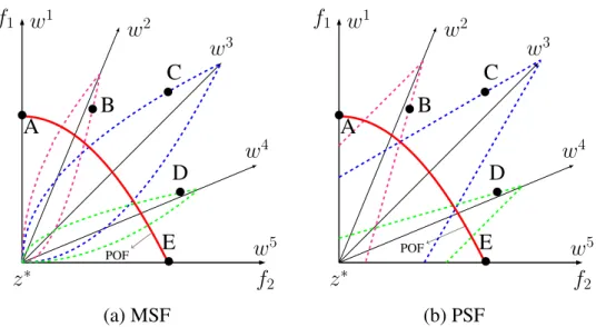
4.2.1 Multiplicative Scalarizing Function (MSF) . . . 59
4.2.2 Penalty-based Scalarizing Function (PSF) . . . 61
4.2.3 Similarities and Differences . . . 62
4.3 Parameter Sensitivity in MSF and PSF . . . 64
4.4 Proposed EA Framework . . . 67
4.4.1 Adaptive Scalarizing Strategy . . . 69
4.4.2 Reproduction Operation . . . 71
4.4.3 Replacement Operation . . . 71
4.5 Experimental Studies . . . 73
4.5.1 Compared Algorithms and Parameter Settings . . . 73
4.5.2 Experimental Results and Analysis . . . 73
4.6 Further Investigations . . . 77
4.6.1 Influence of Mating Selection . . . 77
4.6.2 Influence of Replacement Strategies . . . 78
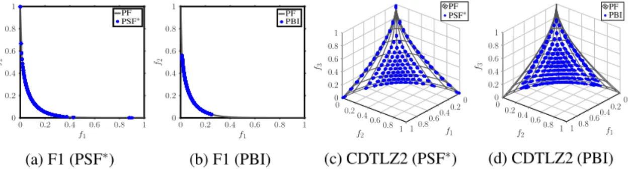
4.6.3 Comparison of PSF and PBI . . . 80
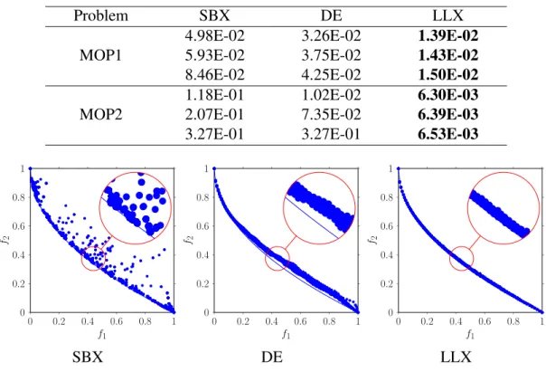
4.6.4 Influence of Recombination Operators . . . 82
4.7 Summary . . . 83
5 EAs for Many-objective Optimization Problems . . . 85
5.1 Introduction . . . 85
5.2 Diversity-based Sorting . . . 87
5.3 DFCS-based Strength Pareto EA . . . 89
5.3.1 Generation of the Reference Direction Set . . . 90
5.3.2 Offspring Reproduction and Objective Normalization . . . 91
5.3.4 Environmental Selection . . . 95
5.3.5 Computational Complexity of SPEA/R . . . 96
5.4 Experimental Studies . . . 97
5.4.1 Experiments on Multiobjective Optimization . . . 97
5.4.2 Experiments on Many-objective Optimization . . . 101
5.5 Further Investigations . . . 108
5.5.1 Comparison of Reference Direction Generation Approaches . . . 108
5.5.2 SPEA/R vs NSGA-III . . . 112
5.5.3 Influence of Fitness Assignment and Niche Preservation . . . 113
5.5.4 Influence of Restricted Mating . . . 115
5.5.5 Peformance of SPEA/R on Problems with More Objectives . . . . 115
5.5.6 Further Discussion . . . 117
5.6 Summary . . . 119
6 A Test Environment for Dynamic Multiobjective Optimization . . . 121
6.1 Introduction . . . 122
6.2 Proposed Test Suites . . . 122
6.2.1 The Proposed Benchmark Generator . . . 122
6.2.2 Test Instances . . . 123
6.2.3 Comparion with Other Benchmarks . . . 131
6.2.4 Discussions . . . 133
6.3 Experimental Studies . . . 133
6.3.1 Performance Metrics . . . 133
6.3.2 Compared Algorithms and Parameter Settings . . . 136
6.3.3 Experimental Results . . . 137
6.3.4 Influence of Variable Linkages . . . 147
6.3.5 Limitations . . . 149
6.4 Summary . . . 149
7 EAs for Dynamic MOPs. . . 151
7.1 Introduction . . . 151
7.2 Proposed SGEA Method . . . 153
7.2.1 Environmental Selection . . . 154
7.2.2 Mating Selection and Genetic Operators . . . 157
7.2.3 Population Update . . . 157
7.2.4 Dynamism Handling . . . 158
7.2.5 Computational Complexity of One Generation of SGEA . . . 161
7.3 Experimental Design . . . 162
7.3.1 Test Problems . . . 162
7.3.2 Compared Algorithms . . . 162
7.3.4 Parameter Settings . . . 164
7.4 Experimental Results . . . 164
7.4.1 Results on FDA and dMOP Problems . . . 164
7.4.2 Results on ZJZ and UDF Problems . . . 170
7.5 Discussions . . . 175
7.5.1 Influence of Severity of Change . . . 175
7.5.2 Study of Different Components of SGEA . . . 177
7.5.3 Influence of Introducing Mutated Solutions . . . 179
7.5.4 Influence of Introducing Random Solutions . . . 180
7.5.5 Further Discussion . . . 182
7.6 Summary . . . 183
8 Conclusions and Future Work. . . 185
8.1 Conclusions . . . 185
8.2 Future Work . . . 187
Bibliography . . . 191
A Appendix MOP Test Problems . . . 206
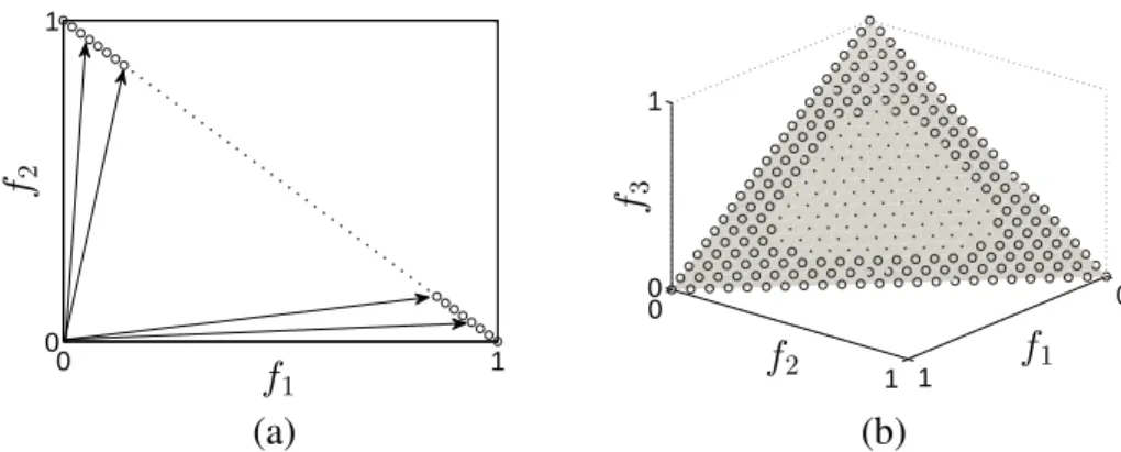
2.1 The flowchart of general MOEAs. . . 13 3.1 Distribution of the extreme weight vectors (circles) and intermediate
weight vectors (black dots): (a) the 2-objective case; (b) the 3-objective
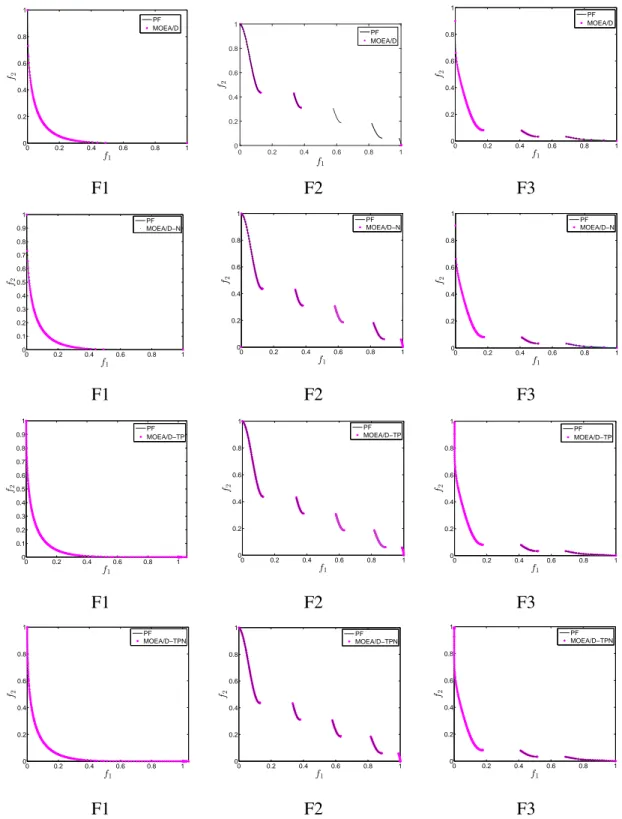
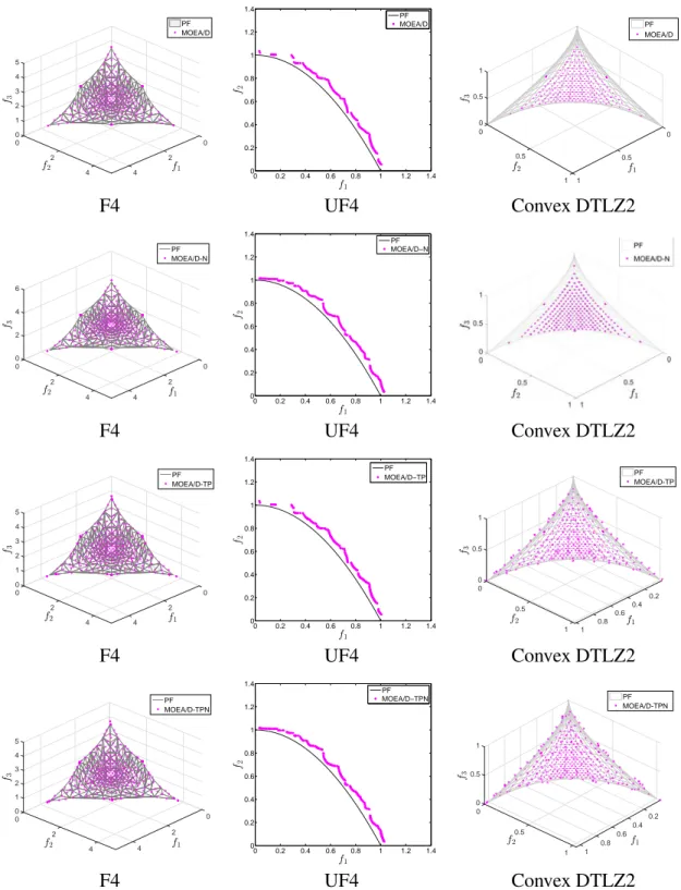
case. . . 32 3.2 PF approximations with the lowest IGD values among 30 runs on F1-F3. . 41 3.3 PF approximations with the lowest IGD values among 30 runs on F4,
UF4 and convex DTLZ2. . . 42 3.4 PF approximations with the lowest IGD values among 30 runs on F1,
F2 and UF4. . . 45 3.5 PF approximations with lowest IGD values among 30 runs on POL,
mF4, F5 and F6. . . 48 3.6 Evolution of the mean IGD values of the test problems: (a) POL, (b)
mF4, (c) F5, and (d) F6. . . 49 3.7 Evolution curves ofDmid andDext on F1, F2, and F3. . . 50
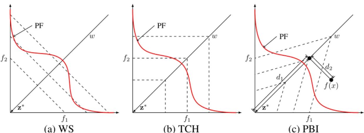
3.8 Influence of TP on population diversity for F2. . . 51 4.1 Illustration of three scalarizing functions on weight vector w, where
dashed lines are contour lines. . . 58 4.2 Illustration of solution distribution in the bi-objective space. Dashed
lines are contours ofL∞scalarizing functions. . . 58
4.3 Contour lines of MSF with differentα values. . . 60 4.4 The improvement region (shaded area) of MSF. . . 60 4.5 Contour lines of MSF withα =0.5 for contour values of 0.4, 0.8, and 1.2. 61
4.6 Contour lines of PSF with differentα values . . . 62 4.7 Contour lines of PSF withα =1.0 for contour values of 0.4, 0.8, and 1.2. 62
4.8 Illustrations of MSF and PSF for maintaining diversity, where dashed
lines are contours. . . 63 4.9 An illustration where MSF (red solid) and PSF (blue dashed) induce
different shapes of contours. . . 63 4.10 Mean IGD values obtained by MSF with differentβ settings. . . 65
4.11 Mean∆pvalues obtained by MSF with differentβ settings. . . 66
4.12 Mean HVD values obtained by MSF with differentβ settings. . . 67
4.13 Mean IGD values obtained by PSF with differentβ settings. . . 68
4.14 Mean∆pvalues obtained by PSF with differentβ settings. . . 69
4.15 Mean HVD values obtained by PSF with differentβ settings. . . 70
4.16 Evolution curve of the mean HVD metric obtained by MSF with differ-entβ settings. . . 70
4.17 Evolution curve of the mean HVD metric obtained by PSF with differ-entβ settings. . . 71
4.18 PF approximations obtained by ten algorithms for MOP1. . . 77
4.19 PF approximations obtained by ten algorithms for MOP5. . . 78
4.20 PF approximations obtained by ten algorithms for MOP6. . . 79
4.21 PF approximations obtained by ten algorithms for MOP9. . . 80
4.22 Mean HVD values obtained by MSF∗with differentδ settings. . . . 81
4.23 Evolution curves of the mean RR obtained by different replacement strategies. . . 81
4.24 PF approximations of PSF∗and PBI over 30 runs on two convex problems. 82 4.25 PF approximations obtained by different recombination operators for MOP1. . . 83
4.26 PF approximations obtained by different recombination operators for MOP2. . . 83
5.1 Nondominated Sorting. . . 87
5.2 DFCS Sorting. . . 88
5.3 Intersections of reference directions and a unit simplex: (a) reference directions on the subsimplexSimp(i); (b) reference directions (with 28 directions generated by 3 layers) in three-dimensional space. . . 91
5.4 Influence of decomposed subregions on environmental selection. The grey area represents the subregion occupied by w2, i.e., Ψ2, and the dashed lines are used to indicated dominatesc. . . 95
5.5 PF approximations for MOP test problems over 30 runs. . . 99
5.6 IGD curves of three algorithms for six MOP problems. . . 100
5.7 Evolution behaviour comparison between SPEA/R and MOEA/D-M2M for three stages on MOP2 and MOP3. Left: 50th generation; middle: 500th generation; right: 1000th generation. . . 101
5.8 Parallel coordinates of final solutions obtained by six algorithms for the 12-objective WFG4 instance. . . 106
5.9 Parallel coordinates of final solutions obtained by six algorithms for the 12-objective WFG5 instance. . . 107
5.10 Parallel coordinates of final solutions obtained by six algorithms for the
12-objective WFG6 instance. . . 107 5.11 Comparison of the population size required by different methods: (a)
the systematic approach andk-layer approach for low-dimensional cases; (b) the two-layer approach andk-layer approach for high-dimensional
cases. . . 108 5.12 Boxplots of the IGD results obtained by algorithms using the SLD and
k-layer approaches for the 3-objective WFG4 instance. . . 111 5.13 Boxplots of the IGD results obtained by SPEA/R using the SLD and
k-layer approaches for the 8-objective WFG4 instance. . . 111 5.14 Parallel coordinates of final solutions obtained by different reference
direction generation methods for the 8-objective WFG4 instance. . . 112 5.15 PF approximations for scaled WFG5 in median and worst cases. . . 113 5.16 The IGD metric against the number of generations for two instances:
SPEA/R (solid); SPEA/R-A (dashed); SPEA/R-B (dotted). . . 114 5.17 Parallel coordinates of final solutions obtained by SPEA/R for WFG
with 20 (a) and 40 (b) objectives. . . 117 5.18 The relative frequency of the number of subregions occupied only by
dominated solutions. . . 118 5.19 The percentage of dominated solutions in every generation of SPEA/R
for 12-objective WFG5. . . 119 6.1 PFs ofJY with different overall shapes: (a)αt=βt =1, At =0.1, and
Wt =3; (b)αt =βt=1, At=0.05, andWt=6; (c) convex or concave
overall shapes withAt=0.05 andWt=6; (d) mixed overall shapes with
At=0.05 andWt=6. . . 124
6.2 PF of JY2 with 21 time windows varying from 0 to 2. For a better
visualization, f1+2tand f2+2tare shown on thexandyaxes, respectively.125
6.3 PS ofJY3 for the first two variables with 6 time windows varying from 0 to 0.5. For a better visualization,x1andx2+tare shown on thexand
yaxes, respectively. . . 126 6.4 PF of JY4 with 11 time windows varying from 0 to 2. For a better
visualization, f1+t and f2+tare shown on thexandyaxes, respectively. 127
6.5 PF ofJY5 with 21 time windows varying from 0 to 2. . . 127 6.6 PF of JY8 with 11 time windows varying from 0 to 1. For a better
visualization, f1+2tand f2+2tare shown on thexandyaxes, respectively.129
6.7 PF ofJY9 with 12 time windows varying from: (a) 0.5 to 1; (b) 1 to 1.5. For a better visualization, f1+2t and f2+2t are shown on the xandy
6.8 An example of the obtainedPF∗far from thePF. . . 134 6.9 Illustration of performance measure against time. . . 135 6.10 The tracking of the IGD values obtained by six algorithms for timet
from 0 to 2. . . 143 6.11 PFs ofJY2 with lowestIGDvalues obtained by six algorithms for time
tfrom 0 to 4. . . 146 6.12 PFs ofJY5 with lowestIGDvalues obtained by six algorithms for time
tfrom 0 to 2. . . 146 6.13 PFs ofJY8 with lowestIGDvalues obtained by six algorithms for time
tfrom 0 to 2. . . 147 7.1 The flowchart of SGEA with the steady-state procedure (in light green)
and generational procedure (in light grey). . . 155 7.2 Evolution curves of averageIGDvalues for eight problems withτt=10
andnt =10. . . 171
7.3 Obtained PFs for four problems withτt=10 andnt=10. . . 172
7.4 Evolution curves of average IGD values for twelve variable-linkage
problems withτt =10 andnt=10. . . 174
7.5 PFs of dMOP3 (τt =10 and nt =10) obtained by SGEA-v2 over 31
time steps. . . 181 7.6 Comparison of IGD curves between dCOEA and SGEA-v2 for dMOP3
3.1 Test Instances . . . 39 3.2 Best, median and worst IGD and HV values of the four algorithms on
the test problems . . . 43 3.3 Best, median and worst IGD and HV values of the peer algorithms on
four test problems . . . 45 3.4 Extra Test Instances . . . 46 3.5 Best, median and worst IGD, HV and T (seconds) values of the three
algorithms on the extra test problems . . . 47 3.6 IGD values obtained by MOEA/D-TPN with differentMr settings for
the instances F1 and F3 . . . 51 3.7 IGD values obtained by MOEA/D-N with different σshare settings for
the instances F2 and UF4 . . . 52 3.8 Population size settings for three algorithms . . . 53 3.9 Best, median and worst IGD values of three algorithms on POL and mF4 53 4.1 Best, median, and worst∆pvalues obtained by different algorithms . . . . 74
4.2 Best, median, and worst HVD values obtained by different algorithms . . 75 4.3 Best, median and worst values of∆pand HVD obtained by PSF∗and PBI 82
4.4 Best, median and worst HVD values obtained by MSF with different
recombination operators . . . 83 5.1 Mean and stand deviation IGD and HV values on MOP problems . . . 98 5.2 Population size for different algorithms using thek-layer approach . . . . 103 5.3 Mean and standard deviation IGD values obtained by six algorithms for
WFG problems . . . 104 5.4 Mean and standard deviation HV values obtained by six algorithms for
WFG problems . . . 105 5.5 Population size settings for SLD and k-layer for different numbers of
objectives . . . 109 5.6 CentredL2-discrepancy values of SLD and k-layer for different
5.7 Statistical difference between SPEA/R and two variants . . . 114
5.8 Mean and standard deviation HV values obtained by SPEA/R with dif-ferentKvalues for four WFG problems . . . 116
6.1 Comparison of characteristics involved in some existing test suites for EDMO . . . 132
6.2 MeanSmetric values, standard deviations and individual ranks for bench-marksJY1−JY10 . . . 138
6.3 MeanRMSmetric values, standard deviations and individual ranks for benchmarksJY1−JY10 . . . 139
6.4 Mean IGDmetric values, standard deviations and individual ranks for benchmarksJY1−JY10 . . . 140
6.5 Mean R(IGD)metric values, standard deviations and individual ranks for benchmarksJY1−JY10 . . . 141
6.6 Performance rankings on four metrics for benchmarksJY1−JY10 . . . . 145
6.7 Influence of variable linkages on algorithms’ performance . . . 148
7.1 Mean and standard deviation values of S metric obtained by five algorithms165 7.2 Mean and standard deviation values of MS metric obtained by five algo-rithms . . . 166
7.3 Mean and standard deviation values of IGD metric obtained by five al-gorithms . . . 167
7.4 Mean and standard deviation values of HVD metric obtained by five algorithms . . . 168
7.5 Mean and standard deviation values of HVD metric obtained by five algorithms on ZJZ and UDF problems . . . 173
7.6 Mean and standard deviation values of HVD metric obtained by five algorithms with different values ofnt . . . 176
7.7 Performance Comparison of SGEA Variants . . . 178
7.8 S, MS and IGD values of SGEA-v1 for FDA1 and FDA2 . . . 180
7.9 S, MS and IGD values of SGEA-v2 for dMOP3 . . . 181
7.10 Comparison between dCOEA and SGEA-v2 on dMOP3 . . . 182
Algorithms
ACD Adaptive Constrained Decomposition AGR Adaptive Global Replacement
dCOEA Dynamic Competitive-cooperative Coevolutionary Algorithm DFCS Diversity First and Convergence Second
DU Distance-based Update EA Evolutionary Algorithm
MOEA Multiobjective Evolutionary Algorithm
MOEA/D Multiobjective Evolutionary Algorithm Based on Decomposition MSF Multiplicative Scalarizing Function
PBI Penalty-based Boundary Intersection
PICEA-g Preference-inspired Coevolutionary Evolutionary Algorithm PSF Penalty-based Scalarizing Function
SDE Shift-based Density Estimation
SGEA Steady-state and Generational Evolutionary Algorithm SPEA/R Strength Pareto Evolutionary Algorithm Based on Reference STM Stable Matching
TCH Weighted Tchebycheff
TPN Two-Phase and Niching Strategy
Acronyms
DCI Diversity Comparison Indicator DE Differential Evolution
DMOP Dynamic Multiobjective Problem
EDMO Evolutionary Dynamic Multiobjective Optimization EMO Evolutionary Multiobjective Optimization
FDA Farina-Deb-Amoto test suite GD Generational Distance
HV Hypervolume
HVD Hypervolume Difference IGD Inverted Generational Distance JY Jiang-Yang test suite
MaOP Many-objective Optimization Problem MOP Multiobjective Optimization Problem
MS Maximum Spread
NS Nondominated Set
PCI Performance Comparison Indicator PF Pareto Front
PS Pareto Set
R(PM) Robustness of Performance Measure RMS Revised Maximum Spread
SBX Simulated Binary Crossover UDF Unconstrained Dynamic Functions WFG Walking-Fish-Group test suite ZDT Zitzler-Deb-Thiele test suite
Symbols
∆p Hausdorff indicator
Ωf objective space
Ωt time space
Ωx search space
Pareto dominance relation σshare niche radius in niche sharing
∆(c) the size of improvement region B(i) the neighborhood of subproblemi Dext crowdedness for extreme populations
Dmid crowdedness for intermediate populations
fi thei-th objective value
gen generation counter
HMk the number of reference directions M the number of objectives
MaxGen the maximum number of generations N population size
n the number of decision values
nr the maximum number of replaceable individuals in MOEA/D
pm crossover probability
ri thei-th component of nadir point
wi thei-th component of a weight vector
xi thei-th decision variable
Introduction
Many real-life problems ranging from engineering to economics involve multiple objec-tives to be optimized [46]. For example, the decision on the purchase of a flight ticket depends on departure/arrival places and time, flight duration, safety, airline service, and the cost. The objectives are often in conflict with each other, and problems having this con-flicting nature are referred to multiobjective optimization problems (MOPs). As a result, there is no single solution that could minimize or maximize all the objectives simultane-ously. Instead, the optima of an MOP are a set of trade-off solutions that compromise objectives, known as the Pareto set (PS) in the decision space and Pareto front (PF) in the objective space. Solutions in the PS are incomparable as each of them represents a certain compromise between the objectives.
Mimicking the process of nature evolution, i.e., the survival of the fittest [38], evo-lutionary algorithms (EAs) are an important method applied to solve MOPs [34]. The popularity of using EAs for multiobjective optimization is due to the following advan-tages. First, EAs do not require much knowledge about problem properties, e.g., continu-ity and differentiabilcontinu-ity, compared with traditional mathematical programming methods [158]. Second, EAs can provide a set of solutions by employing a population of candi-dates and evolving them simultaneously in a single run. Third, EAs have the ability to handle complex search environments, e.g., the search space is very large or has discon-nected regions.
MOPs are a general term to refer to problems with at least two objectives. However, different MOPs may have different problem properties, resulting in distinct optimization difficulties for EAs. Thus, it is not trivial to classify MOPs into different categories ac-cording to their problem properties. In the community of evolutionary computation, there are three popular subcategories of MOPs: (static) MOPs, (static) many-objective opti-mization problems (MaOPs), and dynamic MOPs (DMOPs).
MOPs or static MOPs are often related to problems with two or three objectives. After decades of development, the research on MOPs has achieved fruitful results. Theoretical
foundation and algorithm design have been deeply studied. Despite that, some work re-lated to multiobjective optimization has not been fully understood. Wider problem types should be investigated and more improvements are expected to be made toward existing EAs.
objective problems differentiates from MOPs in the number of objectives. Many-objective problems involve more than three Many-objectives. Due to the increase in the number of objectives, existing EAs that are originally designed for MOPs suffer from significant loss of selection pressure and their performance deteriorates dramatically [43]. In order to make EAs applicable to many-objective problems, effective selection methods are needed to increase selection pressure during the search.
Dynamic MOPs are a kind of MOPs in which objective functions and/or constraints change over time. Due to environmental changes in dynamic MOPs, feasible solutions can become infeasible, and promising ones can become unexpectedly poor. The con-sequences of dynamic environments give rise to new challenges to EAs. However, the research on evolutionary dynamic multiobjective optimization is now at the very early stage. There is a lack of diverse test environments, suitable performance metrics, and ef-fective algorithms in the field of dynamic multiobjective optimization. These open issues need to be addressed in order to promote the development of this field.
This chapter is organized as follows. First, the motivation of undertaking this research is explained. Thereafter, the main objectives of this research are stated, followed by an outline of contributions. Finally, the overall structure of this thesis is provided.
1.1
Motivation
Evolutionary multiobjecitve optimization (EMO) in static and dynamic environments is a challenging research topic because it not only involves the simultaneous optimization of multiple complex objectives, but also requires multiobjective EAs (MOEAs) to be capa-ble of addressing many issues related to different optimization environments. There have been great advances made in multiobjective optimization, many-objective optimization and dynamic multiobjective optimization in recent years. However, the ability and appli-cability of EAs to various optimization environments have not yet been well understood.
The primary motivation of this work is to extend EAs’ applicability to a wide variety of MOPs, including both static and dynamic optimization environments, and facilitate the-oretical foundations for dynamic multiobjective optimization. The following paragraphs are devoted to explaining the incentive of this research work in detail.
A large number of EAs have been proposed for multiobjective optimization, and they have been shown to be very promising for solving a variety of MOPs [43, 120, 188]. Among them, decomposition-based EAs [188] are a popular class of methods and have
become a baseline algorithm by winning the continuous multiobjective optimization com-petition in the 2009 IEEE Congress on Evolutionary Computation [190]. However, some recent studies have shown that the decomposition-based EAs could be influenced by PF geometries of MOPs, particularly when optimizing MOPs with complex PFs [139]. As a result, they fail to provide a good coverage and distribution of solutions. This issue needs to be addressed in order to improve the applicability of this kind of EAs.
Scalarizing functions are widely used in multiobjective optimization. Scalarizing func-tions are an important tool to convert a MOP into a number of MOPs or sing-objective problems [188]. Through conversion, the MOP becomes easier to be handled. Despite great success, scalarizing functions are not yet fully understood. A particular question related to scalarizing functions is: how do they affect the search behaviour of EAs? To answer this question soundly, a deep investigation is required.
Many-objective problems are more challenging than MOPs for EAs. Due to the in-crease in the number of objectives, Pareto dominance relation becomes ineffective to dis-criminate solutions, leading to a dramatical loss of selection pressure during the search [43]. Facing this issue, a natural question arises – is there any other effective method in place of the Pareto dominance based selection method? This is an interesting question and worthwhile of investigation.
Dynamic MOPs frequently appear in real-world applications [55]. This kind of prob-lems brings new challenges to EAs. Dynamic test probprob-lems play an important role in deeply studying and understanding dynamic environments. They are also helpful for al-gorithm design and development. However, in the field of dynamic multiobjective op-timization, there is a lack of standard test environments that can be used to deeply and comprehensively study the challenges caused by dynamic environments and assess EAs’ ability to deal with these challenges. Therefore, standard test problems are desirable in order to advance the development of EAs for dynamic MOPs.
While EAs have been shown to be powerful and efficient optimizers for static MOPs, they encounter difficulties in solving dynamic MOPs. Due to environmental changes, EAs are very likely to lose population diversity, and nondominated solutions discovered in the previous environment may be no longer nondominated [61]. The changing environments require EAs to be capable of maintaining diversity, detecting changes, and converging quickly. In other words, a good EA should be able to track the changing PS/PF and provide a set of well-diversified solutions for each environmental change. In this research field, there is a great need of good EAs that are able to handle dynamic environments and serve as baseline algorithms for algorithm comparison.
1.2
Objectives
The overall purpose of this work is to make EAs applicable to various MOPs with different problem characteristics and optimization difficulties. To accomplish the overall objective some specific objectives are proposed:
• A review of decomposition-based EAs for MOPs with complex PFs will be con-ducted. This will result in a further and extensive understanding of strengths and weaknesses of decomposition-based EAs when solving this kind of problems. Novel techniques will be proposed to alleviate or overcome the observed drawbacks, and these new techniques will be examined on complex-PF MOPs and compared with other peer methods to show the effectiveness.
• EAs with scalarizing functions for MOPs will be systematically studied. First, po-tential drawbacks of existing scalarizing functions will be analysed qualitatively. In view of the drawbacks of incorporating these scalarizing functions into EAs for MOPs, new scalarizing functions will be proposed. These new scalarizing func-tions will be studied quantitatively and qualitatively. They will also be integrated into EAs to solve MOPs, and experimental studies will be carried out to show the superiority of the proposed methods.
• Different selection methods will be investigated in the field of many-objective op-timization. Particularly, the difference between diversity-biased and convergence-biased selection methods will be studied. An extensive experimental study will be conducted to identify the most suitable one from these two kinds of selection methods for many-objective optimization. The selection method identified will be combined with new strategies to form a new algorithm for many-objective optimiza-tion. The new algorithm will be validated through fair comparisons with state of the arts.
• An extensive investigation and thorough analysis in test suites for dynamic multi-objective optimization will be carried out to identify the common dynamic features among existing test suites. Based on the analysis, new and representative dynamic characteristics that are rarely considered will be assessed, and this will lead to the development of a new dynamic test suite. The new test suite will be used to study the ability of EAs to handle environmental changes. The strengths and weaknesses of some EAs for dynamic multiobjective optimization will be summarized.
• On the basis of the above testing, a new EA framework will be developed for dy-namic multiobjective optimization. The new EA will take the advantage of steady-state EAs in promoting convergence and the advantage of generational EAs in main-taining diversity, thereby having the ability to react to changes quickly and search
new PFs effectively. The proposed EA will be examined on a wide range of test problems, and its performance will be validated by comparing existing popular dy-namic multiobjective optimizers.
1.3
Contributions
The following summarises the main contributions of this thesis:
• A new two-phase search method and a niche-guided selection method are inte-grated into decomposition-based EAs for solving MOPs with complex PFs (Chap-ter 3). The popular decomposition-based EA, e.g., MOEA based on decomposition (MOEA/D) [188], maintains diversity on the assumption that uniform weight vec-tors provide a set of uniformly-distributed solutions. However, this assumption hardly holds when the PF to be approximated is irregularly shaped, e.g., MOEA/D is likely to generate duplicate solutions if the PF has disconnected segments. More-over, MOEA/D uses a simple solution selection method for mating and replacement without considering the density of solutions, which can easily lead to overexploita-tion/underexploitation in some regions, particularly for complex PFs. In view of these drawbacks, a two-phase search method is proposed to divide the search into two phases, where the first phase is devoted to a coarse search and the second phase helps refine the solutions obtained from the first phase and improve their distribu-tion. A niche-guided selection is introduced to reduce the chance of selecting solu-tions from overcrowded regions and enhance the search in underexplored regions, thereby guaranteeing good population diversity during the search.
The two-phase and niche-guided (TPN) strategy is tested on a number of irregu-lar MOPs with different PF characteristics, e.g., sharp-peak/long-tail PFs, discon-nected PF segments and multimodal PFs. The experimental study has shown the effectiveness of TPN in improving MOEA/D for solving complex MOPs. Further-more, MOEA/D with TPN has been compared with other peers and state-of-the-art algorithms, demonstrating that it is very promising for finding well-converged and uniformly-distributed solutions for MOPs with various and complex PFs.
• New scalarizing functions (i.e., the multiplicative scalarizing function (MSF) and penalty-based scalarizing function (PSF)) are introduced for hard MOPs and their impact on search behaviour is deeply investigated (Chapter 4). Unlike the commonly-used existing scalarizing functions, e.g., the weighted sum (WS), the weighted Chebycheff (TCH) and the penalty-based boundary intersection (PBI) [188], which are difficult to maintain the balance between diversity and convergence for hard search environments, the MSF and PSF can induce adjustable improvement regions
so that diversity can be well controlled during the search. Also, MSF and PSF pro-mote the similar size of improvement regions. As a result, all the solutions to the subproblems can make equally good progress during the evolution. Besides, an ef-ficient EA based on the proposed scalarizing functions (eMOEA/D) is proposed for multiobjective optimization.
The eMOEA/D algorithm has been investigated on a number of difficult MOPs where local attractors can cause evolutionary stagnation. Compared with nine state-of-the-art scalarizing-based or decomposition-based algorithms, eMOEA/D is more capable of balancing diversity and convergence, thereby producing high-quality so-lutions at the end of the search. This implies the usefulness of the new scalarizing functions in dealing with hard MOPs.
• A novel diversity-first-and-convergence-second (DFCS) selection approach is pro-posed to handle many-objective optimization (Chapter 5). Unlike most existing Pareto-based EAs that approximate the PF in a convergence-first-and-diversity-second manner, DFCS considers diversity as the first selection criterion. This way, the loss of selection pressure resulting from Pareto dominance can be rescued by the increase of diversity emphasis. On the basis of DFCS, a new EA, called SPEA/R, is introduced to deal with many-objective problems. SPEA/R employs a set of di-verse weight vectors to partition the objective space into a number of subspaces and uses a Pareto-based method to do fitness assignment. As a result, SPEA/R makes it possible to use Pareto dominance in many-objective optimization.
The effectiveness and promise of SPEA/R has been verified on both MOPs and many-objective problems. This refutes the common belief that Pareto dominance is ineffective in many-objective optimization. An interesting finding from empirical studies is that diversity may be more important than convergence in the case of optimizing many-objective problems considered in this thesis.
• A new test suite (i.e., JY) is developed for dynamic multiobjective optimization (Chapter 6). The JY test suite is proposed to meet the need of standard test envi-ronments in the field of dynamic multiobjective optimization. Unlike some existing test suites, JY contains test problems with typical and diverse dynamic characteris-tics, e.g., mixed PFs in terms of convexity and concavity that change over time, and non-monotonic and time-varying linkages between variables instead of static mono-tonic variable-linkage used in the literature. The JY test suite plays an important role in furthering theoretical analysis and widening insights in the understanding of dynamics involved in changing optimization environments.
The JY test suite has been adopted to study and assess the ability of different MOEAs to deal with dynamic environments. According to the used performance
metrics including both existing and new ones, JY is able to facilitate a comprehen-sive understanding of MOEAs in response to environmental changes. Therefore, JY is a promising toolbox for the research and development of dynamic multiobjective optimization.
• A new EA based on the combination of generational and steady-state search meth-ods is suggested for dynamic multiobjective optimization (Chapter 7). In the field of dynamic multiobjective optimization, an important topic is to design effective and efficient EAs that can handle dynamic environments well. In other words, EAs should be able to maintain diversity and convergence well whenever there is an environmental change. The proposed EA (i.e., SGEA) is inspired by the fast con-vergence of steady-state EAs and the good diversity maintenance of generational EAs. Unlike most existing approaches, SGEA detects and reacts to changes in a steady-state manner and maintains population diversity in a generational manner. It also uses history information and the new information about the population to relocate the current population so that the population is close to the optima in new environments. This way, SGEA is easy to track the change of the PF and solve the current problem before new environments arrive.
The SGEA has been studied on a wide variety of test suites with different character-istics. Empirical studies have revealed that SGEA reacts to environmental changes faster and more stably than its competitors. SGEA works generally well on most of the considered test problems. This work will attract more research interests in dynamic multiobjective optimization.
1.4
Overview
The main purpose of this work is to investigate the suitability of EAs for solving different kinds of MOPs and make subsequent improvements on the applicability of EAs for these MOPs. As the performance of EAs is very problem-specific, the thesis is organized such that (roughly) each chapter covers one kind of MOPs and/or an EA designed specifically for this kind of MOPs. Thus, there may be a lack of strong links between some chapters. Generally, however, Chapters 3, 4, and 5 can be in one group and are devoted to studying static MOPs with different characteristics, whereas Chapters 6 and 7 are another group which focuses on dynamic MOPs. Static MOPs from Chapter 3 to Chapter 5 have an in-creasing level of optimization difficulties in the first group, and all the corresponding EAs designed use the same idea of decomposition for dealing with these increasingly difficult MOPs. The second group starts from constructing dynamic test environments to compare existing EAs in handling dynamic characteristics (which are presented in Chapter 6), and
ends with designing a new EA (in Chapter 7) to overcome the drawbacks identified by the previous chapter.
To be specific, the thesis is organized as follows.
First, in Chapter 2, background knowledge and related work are presented. This chap-ter introduces three main topics related to evolutionary multiobjective optimization, i.e., static multiojective optimization, many-objective optimization and dynamic multiobjec-tive optimization. In each topic, related work is described, including basic concepts, test suites, mainstream approaches, and performance metrics.
Chapter 3 starts with the motivation of improving decomposition-based EAs for solv-ing MOPs with complex PFs. Then, a new two-phase search strategy and a niche-guided selection strategy are suggested to be used in decomposition-based EAs. After that, ex-tensive experiments are carried out to verify the effectiveness of the proposed method, followed by deep sensitivity analysis.
Chapter 4 presents two new scalarizing functions after the illustration of potential drawbacks of existing scalarizing functions. Based on the new scalarizing functions, an efficient MOEA/D (i.e., eMOEA/D) is suggested. Broad algorithm comparisons are then conducted to show the promise of the proposed algorithm, followed by a further investi-gation into the impact of different strategies.
In Chapter 5, a new diversity-first-and-convergence-second (DFCS) selection method is introduced to overcome the disadvantages of convergence-first based methods. With the aid of DFCS and reference directions, a new optimizer, i.e., SPEA/R, is then suggested. Experimental studies are conducted on both multiobjective and many-objective optimiza-tion. Finally, further investigations are made to show the strengths and weaknesses of SPEA/R and peer methods.
Chapters 6 and 7 focus on addressing open issues in the field of dynamic multiobjec-tive optimization. Specifically, Chapter 6 attempts to construct a diverse dynamic multiob-jective test environments by introducing a new test-bed consisting of diverse and typical dynamic characteristics. The test bed is then used to examine the performance of some ex-isting dynamic optimizers, providing a deep understanding of dynamics in time-changing environments.
Based on the analysis of empirical results provided in the previous chapter, Chapter 7 introduces a dynamic EA to deal with dynamic environments. The proposed EA, i.e., SGEA, is tested and evaluated on various test environments, and general concerns about this algorithms is discussed.
Chapter 8 summarizes the work presented in this thesis and points out contributions to corresponding research field. Future research directions are also outlined.
Background
This chapter is devoted to presenting preliminary knowledge of this thesis. The structure of this chapter is organized as follows. Section 2.1 describes related work on evolutionary multiobjective optimization, including problem definition and evolutionary approaches. Section 2.2 reviews the work on evolutionary many-objective optimization, followed by a review of the research on evolutionary dynamic multiobjective optimization (EDMO) in Section 2.3. Section 2.4 summarizes this chapter.
2.1
Evolutionary Multiobjective Optimization
2.1.1
Multiobjective Optimization Problems
2.1.1.1 Problem Definition
A multiobjective optimization problem (MOP) can be mathematically described as fol-lows:
min f(x) =f1(x),f2(x), . . . ,fM(x) T s.t. x∈Ωx,
(2.1)
where Ωx ⊆Rn is the decision space and x = (x1, . . . ,xn)T is a candidate solution. f :
Ωx7→Ωf ⊆RM containsMobjective functions, andΩf is the attainable objective space.
In this thesis, we only focus on MOPs with box constraints. That is,Ωxcan be written as
Ωx=∏ni=1[li,ui], wherelianduiare upper and lower bounds ofxifor alli=1, . . . ,n.
More often than not, the objectives of the problem (2.1) are in conflict with each other. This means, any improvement in one objective will inevitably result in deterioration of another objective. Thus, no single solution exists that makes all the objectives reach their optima. Instead, the optimality of the problem (2.1) consists of a set of trade-off solutions (called Pareto-optimal set) that compromise all the objectives. Concepts related to Pareto optimality [46] are described in the next section.
2.1.1.2 Basic Concepts
Definition 2.1. A solution x is said to dominate another solution y if x is not worse than y in all objectives and is better than y in at least one objective. This is denoted xy. Definition 2.2. A solution x∗ is said to be Pareto optimal if no another solution x in the decision space satisfies xx∗.
Definition 2.3. The Pareto-optimal set (PS) is a set of Pareto-optimal solutions, i.e., PS={x∈Ωx|x is Pareto optimal}.
Definition 2.4. The Pareto-optimal front (PF), the image of PS in the objective space, is defined as,
PF ={f(x)∈Ωf|x∈PS}.
Definition 2.5. The nondominated set (NS) of a set S is a subset of S, i.e., NS ⊂S, and consists of all the solutions that cannot be dominated by any other solution in S. NS is expressed as
NS={s∈S|∄t∈S,ts}.
The above definitions are basic concepts in the field of multiobjective optimization and will be frequently used throughout the thesis.
2.1.1.3 Test Suites
Many real-world optimization problems share various common features. Using artificial test suites as a representative of these common features would make it possible to as-sess different approaches in a much broader context than the usual empirical set for a single application. Besides, artificial test suites also allow to ease theoretical analysis of algorithms. So far, a number of test suites focusing on different types of features have been proposed. In the following, we briefly introduce several test suites that are used for continuous multiobjective optimization.
ZDT Test Suite ZDT [200] is one of the earliest test suites used in multiobjective op-timization. This test suite contains six biobjective problems with different char-acteristics, such as convex or concave PFs, continuous or discontinuous PFs, and unimodal or multimodal PFs.
DTLZ Test Suite The DTLZ [48] test suite is developed to meet the need of scalable test problems where the number of objectives can be easily scaled up. This test suite has nine instances. DTLZ has various features, such as multimodality and disconnectivity. There are also two instances that have inequality constraints.
WFG Test Suite The WFG [82] test suite contains nine distinctive problems, each of which has one or several typical characteristics. This test suite is constructed in view of limitations of the ZDT and DTLZ test suites. In this test suite, more features like mixed PF shapes, degeneration of PFs, biases, deception, and dependencies between variables, are recommended to be used for performance assessment. LZ Test Suite The LZ [120] test suite features nonlinear correlation between variables,
resulting in problems having complicated PS shapes. In practice, LZ test problems can specify arbitrary PS shapes where dependencies between variables can be ad-justed to control the difficulty of convergence. Following this idea, Zhang et al. [190] proposed a test suite of 23 test problems for IEEE Congress on Evolution-ary Computation (IEEE CEC2009)competition, in which more characteristics like constraints and deceptive search spaces are recommended.
MOP Test Suite The MOP [127] test suite is an extension of ZDT and DTLZ but more difficult than its predecessors. It originally has seven problems, each of which has local attractors on the PF. Due to the existence of these local attractors, the MOP problems cannot be solved well by many existing approaches, such as NSGA-II [41] and MOEA/D [188]. Considering the lack of three-objective problems with local attractors in intermediate regions of the PF, Jiang et al. [95] have recently added two more instances to this test suite.
In addition to the above-mentioned test suites, there are also another kinds of test suites. The OKA [135] test suite is a set of problems having complicated PSs, which are constructed through a series of transformations. TYP-MOP [31] is a set of truly dis-connected multiobjective problems where the true PF and PS are in the form of multiple disconnected segments and has been used to examine algorithms’ ability to deal with dis-connectivity. Chenget al. [29] proposed a set of test problems for large-scale multi- and many-objective optimization.
2.1.2
Related EAs
2.1.2.1 Introduction
EAs belong to the class of randomized search heuristics that mimic evolution by natural selection. Multiobjective optimization EAs (MOEAs) extend the applicability of EAs to solving MOPs. Over the past twenty years, there have been increasing research interests in the design of MOEAs for solving MOPs. This is mainly because MOEAs have sev-eral advantages over other optimization methods like mathematical programming. First, MOEAs have low requirements on problem characteristics, e.g., differentiability, and they
can deal with large and complex search spaces. Second, MOEAs can be used in the sit-uation that there are not enough computational resources in terms of money, time, or knowledge to construct a problem-dependent algorithm [15]. Third, MOEAs can provide a set of trade-off solutions close to the PF/PS in a single run, whereas other mathematical approaches like normal boundary intersection [39] can compute only one solution at a time.
It is widely accepted that if no preference information is provided, MOEAs are ex-pected to reach the following main optimization goals when approximating the PF.
• The approximation should be as close to the PF as possible. In other words, MOEAs should provide good convergence performance.
• The approximation solutions should be well-diversified across the PF. That is, MOEAs should provide a good distribution of solutions.
• The approximation should cover the PF well. That means, MOEAs should spread solutions widely over the PF.
The first goal often refers to convergence whereas the second and the third are related to diversity. Therefore, convergence and diversity are widely used to assess and measure the performance of MOEAs. They are generally assumed to be conflicting in EMO, and designing MOEAs is to reach the balance between convergence and diversity. Apart from these goals, in practice MOEAs are also required to have low computational complexity. This makes much sense if there are very limited computational resources.
2.1.2.2 General MOEA Framework
A general MOEA framework is illustrated in Fig. 2.1. MOEAs start with an initial popu-lation of candidate individuals. Very often, the initial popupopu-lation is generated in a random manner. However, if we have some knowledge about the characteristics of a good so-lution, it is wise to use this information to create the initial population. The population evaluation provides solutions with the exact objective values. The environmental selec-tion is intended to preserve the best soluselec-tions in terms of convergence and diversity for the next generational evolution. The population reproduction generates an offspring pop-ulation. The population evaluation, environmental selection and population reproduction run in turn until the stopping criterion is met.
According to the selection strategies used in the environmental selection, MOEAs can be classified into different categories. The following sections provide a broad overview of several main categories of MOEAs proposed in the literature.
Start Population Initialization Population Evaluation Environmental Selection Population Reproducation Stopping Criterion Stop yes no
Fig. 2.1 The flowchart of general MOEAs.
2.1.2.3 Pareto-based Approaches
Pareto-based MOEAs employ the (weak) Pareto-dominance relation (i.e., “”) [46], a kind of notion that defines a partial order in the objective space, to discriminate individuals in the population.
After decades of effort, a large number of Pareto-based MOEAs have been proposed. The multiobjective genetic algorithm (MOGA) [56] is generally considered the first MOEA that applies the concept of Pareto-based selection for mulitobjective optimization. Follow-ing the idea of MOGA [56], some popular MOEAs with Pareto-based selection emerged, including the niched Pareto genetic algorithm (NPGA) [80] and the nondominated sorting genetic algorithm (NSGA) [155]. These algorithms established the utility of MOEAs for solving MOPs. Then, new MOEAs, such as the strength Pareto evolutionary algorithm (SPEA) [203], Pareto envelope based evolutionary algorithm (PESA) [35] and the Pareto archived selection algorithm (PAES) [103], verified the importance of elitism, diversity maintenance and external archiving. These algorithms are commonly referred to as
first-generation. In the early 2000s, some second-generation algorithms were developed, and many of them are an updated version of their first-generation counterparts, e.g., NSGA-II [41], SPEA2 [202] and PEAS-II [36].
Pareto-based selection in MOEAs often has two stages. In the first stage, the popula-tion is ranked into different fronts. Solupopula-tions in the same front usually have the same rank value. The rank assignment can be conducted by dominance rank [155], dominance count [56] or dominance strength [202, 203]. In the second stage, each solution from the same font is assigned a density value. The density of solutions can be estimated by niching and fitness sharing [56, 80], gridding [103], or crowding distance [41]. Density information is used because it can help preserve solutions in sparse areas. Usually, solution ranking is considered the first criterion for solution selection, while solution density is the second criterion. The first criterion can promote population convergence, and the second one helps to maintain good population diversity.
2.1.2.4 Decomposition-based Approaches
Decomposition-based MOEAs, such as multiple single objective Pareto sampling (MSOPS) [83] and cellular multiobjective genetic algorithm (C-MOGA) [131], are a popular class of metaheuristics for EMO. They decompose an MOP into a number of subproblems1 and simultaneously solve them in a collaborative manner. The MOEA based on decom-position (MOEA/D) [188] is a representative of this class of metaheuristics. MOEA/D decomposes an MOP by scalarizing functions (or termed decomposition approaches in some works [188]) into a set of subproblems, each of which is associated with a search di-rection (or weight vector) and assigned a candidate solution. In every generation, parents from a mating pool are selected to generate an offspring solution for each subproblem. Then, the offspring replaces certain existing solutions if it achieves better scalarizing val-ues.
There are three popular scalarizing functions used for decomposition in decomposition-based approaches, which are listed as follows:
(a) Weighted Sum (WS) Method[188]
Assume that w= (w1, . . . ,wm)T is a weight vector where all components are
non-negative and should satisfy ∑m
i=1wi = 1. The WS method defines the following
single-objective problem:
min gws(x|w,z∗) =∑mi=1(wi|fi(x)−z∗i|)
s.t. x∈Ωx.
(2.2)
1Note that, subproblems can be not only single-objective optimization problems [188] but multiobjective
If necessary, throughout the paper, fi(x)−z∗i should be replaced by(fi(x)−z∗i)/(znadiri −
z∗i)wherez∗i andznadiri are thei-th objective values of ideal point and nadir point found so far [188], respectively. The WS method can obtain a set of PF points by different weight vectors. The method can approximate the PF if it is convex, but will miss some PF points if the PF is nonconvex [188].
(b) Weighted Tchebycheff (TCH) Method[188]
The TCH method converts an MOP into a scalar problem in the following form:
min gte(x|w,z∗) = max 1≤i≤m 1 wi|fi(x)−z ∗ i| s.t. x∈Ωx, (2.3)
where wi =10−4 is used in this method if wi =0. In Eq. (2.3), 1/wi instead of wi is
adopted in order to obtain a set of distributed solutions from a set of uniformly-distributed weight vectors [122]. The TCH method has the advantage in approximating nonconvex PFs compared with the WS method. It has been widely employed as a decom-position approach in MOEA/D variants [90, 120, 122, 175].
(c) Penalty-based Boundary Intersection (PBI) Method[188] The PBI method converts an MOP into a scalar problem as follows:
min gpbi(x|w,z∗) =d1+θd2 s.t. x∈Ωx, (2.4) where d1= k(f(x)−z ∗)T wk kwk , (2.5) d2=kf(x)−(z∗+d1 w kwk)k. (2.6)
In PBI, θ is a user-defined penalty factor. d1 and d2 are the length of the projection
of vector (f(x)−z∗) on the weight vector w and the perpendicular distance from f(x)
tow, respectively. θ is a key parameter for balancing convergence (measured byd1) and
diversity (measured byd2). Recent studies [147] have shown that, when PBI approximates
convex PFs, large diversity is likely to be obtained from minute and large θ values, and smallθ values are beneficial to convergence.
The performance of MOEA/D was compared with the improved nondominated sort-ing genetic algorithm (NSGA-II) in [41] and [120] for MOPs with simple and complicated PSs, respectively, showing that MOEA/D is able to generate the best set of diverse non-dominated solutions close to the PF in all tested cases. Furthermore, the efficiency of MOEA/D was confirmed by winning the unconstrained MOEA competition in the 2009
IEEE Congress on EC (IEEE CEC 2009) [190]. Since then, MOEA/D has attracted in-creasing research interest and various modified versions have been proposed in the liter-ature [86, 127, 139]. Besides, the idea has also been integrated into hybrid algorithms [21, 102, 121, 153].
2.1.2.5 Indicator-based Approaches
The main idea behind indicator-based approaches is that quality indicators are able to quantify the quality of an approximate PF obtained. Indicator-based MOEAs often use quality indicators to guide the search, particularly in the process of environmental selec-tion.
The indicator-based evolutionary algorithm (IBEA) [201] is the first implementation of indicator-based approaches. IBEA compares a pair of candidate solutions by an ar-bitrary indicator. As a result, high-quality solutions are preserved for further evolution. Later, Beume et al. [8] proposed a steady-state MOEA, called SMS-EMOA, based on the hypervolume indicator. In environmental selection, the hypervolume contribution of each candidate solution is computed, and the one with the least hypervolume contribu-tion is excluded from the evolving populacontribu-tion. Hyervolume-based MOEAs have received increasing research interests because hypervolume is the only indicator complying with Pareto dominance. However, a major drawback is that hypervolume is computationally demanding, particularly when the number of objectives is high, which is the case with many-objective optimization.
Apart from hypervolume, other indicators have also been successfully applied in indicator-based approaches. The averaged Hausdorff indicator [151] is used in a number of studies [141, 143] to replace hypervolume in the pursue of a computationally cheap indicator-based MOEA. The R2 indicator [18] has also been suggested to be in place of hypervolume in existing indicator-based MOEAs like SMS-EMOA.
2.1.2.6 Preference-based Approaches
Preference-based MOEAs originate from the fact that the number of Pareto optimal so-lutions may be very large or even infinite and the decision maker may be only interested in preferred solutions instead of the whole solutions. When preference information is provided, the search can be directed toward the region of interest to the decision maker.
Some early attempts on preference-based MOEAs are the studies of [56, 64, 157], in which preference information is used to rank the population. In [47], Debet al.proposed a preference-based MOEA. In this method, the decision maker’s performance information is used to model an approximate value function after every few generations of an MOEA. Then, the constructed value function is used to direct the search to more preferred solu-tions.
In a recent work, Wang et al. [172] have proposed to coevolve a family of prefer-ences simultaneously with a population of candidate solutions, which leads to preference-inspired coevolutionary algorithms (PICEAs). Following this idea, they suggested a real-ization of PICEAs, called PICEA-g, and demonstrated that this method provides highly competitive performance for MOPs.
2.1.3
Performance Assessment
Performance measures are of vital importance to indicate whether an algorithm can achieve the optimization goals mentioned earlier. The following lists some widely used indicators in EMO.
2.1.3.1 Generational Distance
The generational distance (GD) metric [41] is one of commonly-used performance mea-sures in EMO. It meamea-sures how close an approximation is to the true PF. LetPF be a set of uniformly distributed points in the true PF, andPF∗be an approximation of the PF. The GD is calculated as follows: GD= (∑ nPF∗ i=1 diq)1/q nPF∗ , (2.7)
wherenPF∗ =kPFk, diis the Euclidean distance between theith member inPF∗and its
nearest member inPF. Very often,q=2 is used.
2.1.3.2 Inverted Generational Distance
The inverted generational distance (IGD) metric in [183, 192] measures both the con-vergence and diversity of solutions obtained by an algorithm. The IGD is calculated as follows: IGD= ∑ nPF i=1di nPF , (2.8)
where nPF =kPFk, di is the Euclidean distance between theith member in PF and its
nearest member in PF∗. To have a low IGD value, PF∗ must be very close to PF and cannot miss any part of the wholePF.
2.1.3.3 Averaged Hausdorff Distance
Averaged Hausdorff distance (∆p) [151] is a recently developed metric that can somewhat
handle the outlier tradeoff. The metric is calculated as follows:
∆p(PF∗,PF)=max ( ∑ x∈PF dp(x,PF∗) |PF| !p , ∑ x∈PF∗ dp(x,PF) |PF∗| !p) , (2.9)
whered(x,PF)is the distance between the member xofPF∗and the nearest member of PF, andd(x,PF∗)is the distance between the memberx ofPF and the nearest member ofPF∗. In this thesis, p=2 is used.
2.1.3.4 Schott’s Spacing
Schott [150] developed a metric with regard to the distribution of the discovered PF, called the spacing metric (S). S measures how evenly the members in a PF approximation (de-notedPF∗) obtained by an algorithm are distributed, and is computed as:
S=qn 1 PF∗−1∑ nPF∗ i=1 (Di−D)2 D= n1 PF∗ ∑ nPF∗ i=1 Di, (2.10)
where Di is the Euclidean distance between the ith member and its nearest member in
PF∗.
2.1.3.5 Maximum Spread
The maximum spread (MS), first introduced by Zitzler et al. [200], measures to what extent the extreme members (usually boundary points) in PF have been reached. Goh and Tan [60] proposed a modified version of MS by taking into account the proximity of PF∗towardsPF: MS= v u u t1 M M
∑
k=1 " min[PFk,PFk∗]−max[PFk,PFk∗] PFk−PFk #2 , (2.11)where PFk and PFk is the maximum and minimum of the kth objective in PF,
respec-tively; Similarly,PFk∗andPFk∗is the maximum and minimum of thekth objective inPF∗, respectively.
2.1.3.6 Hypervolume
The hypervolume (HV) [203] metric measures the size of the objective space dominated by the approximated solution setSand bounded by a reference pointR= (R1, . . .,RM)T
that is dominated by all points on the PF, and is computed by:
HV(S) =Leb( ∪
x∈S[f1(x),R1]× ··· ×[fM(x),RM]), (2.12)
Based on HV, an alternative indicator is defined as follows:
HV D=HV(PF)−HV(PF∗), (2.13) whereHV Dis called hypervolume difference. Thus, minimization of HVD is equivalent to maximization of HV.
2.2
Evolutionary Many-objective Optimization
2.2.1
Many-objective Optimization Problems
2.2.1.1 Problem Definition
In general, many-objective optimization problems (MaOPs) are an extension of MOPs. There is no agreed definition for MaOPs. However, one thing for sure is that MaOPs are often related to MOPs with more than three objectives, that is,M>3 in Eq. (2.1). Due to the increase in the number of objectives, MaOPs bring about new challenges to MOEAs. A typical challenge is that dominance mentioned earlier becomes less effective and even unable to discriminate solutions. As a result, existing MOEAs specially designed for MOPs cannot induce sufficient selection pressure during the search. MaOPs are signifi-cantly different from MOPs, although both have the same mathematical description.
2.2.1.2 Test Suites
Test problems for many-objective optimization problems should have more than three objectives. It is often desirable that the problems are scalable in terms of the number of objectives, because this can allow a deep investigation into the impact of dimension increase. So far, DTLZ [48] and WFG [82] are top two most popular test suites in many-objective optimization.
There are also some other many-objective problems in the literature. Saxena et al. [148] adapted several DTLZ problems so as to generate redundant objectives which can evaluate dimensionality reduction techniques. Liet al. [115] proposed a test problem for easing the difficulty of visualization in many-objective optimi