for Stream Data Mining
Von der Fakult¨at f¨ur Mathematik, Informatik und Naturwissenschaften der RWTH Aachen University zur Erlangung des akademischen Grades eines
Doktors der Naturwissenschaften genehmigte Dissertation
vorgelegt von
Diplom-Informatiker Philipp Kranen
aus Willich, Deutschland
Berichter: Universit¨atsprofessor Dr. rer. nat. Thomas Seidl Visiting Professor Michael E. Houle, PhD
Tag der m¨undlichen Pr¨ufung: 14.09.2011
Diese Dissertation ist auf den Internetseiten der Hochschulbibliothek online verf¨ugbar.
Abstract / Zusammenfassung 1
I
Introduction
5
1 The Need for Anytime Algorithms 7
1.1 Thesis structure . . . 16
2 Knowledge Discovery from Data 17 2.1 The KDD process and data mining tasks . . . 17
2.2 Classification . . . 25
2.3 Clustering . . . 36
3 Stream Data Mining 43 3.1 General Tools and Techniques . . . 43
3.2 Stream Classification . . . 52
3.3 Stream Clustering . . . 59
II
Anytime Stream Classification
69
4 The Bayes Tree 71 4.1 Introduction and Preliminaries . . . 724.2 Indexing density models . . . 76
4.3 Experiments . . . 87
4.4 Conclusion . . . 98 i
5 The MC-Tree 99
5.1 Combining Multiple Classes . . . 100
5.2 Experiments . . . 111
5.3 Conclusion . . . 116
6 Bulk Loading the Bayes Tree 117 6.1 Bulk loading mixture densities . . . 117
6.2 Experiments . . . 122
6.3 Conclusion . . . 127
7 The Classifier Family: Learn from your Relatives 129 7.1 Introduction . . . 129
7.2 Learning from Relatives . . . 131
7.3 Experiments . . . 141
7.4 Conclusion . . . 150
8 Application: Anytime Classification in HealthNet Scenarios 151 8.1 Scenario and Prototype . . . 152
8.2 Summary . . . 157
9 Anytime Algorithms on Constant Streams 159 9.1 Introduction . . . 160
9.2 Novel Approaches for Constant Data Streams . . . 161
9.3 Experiments . . . 169
9.4 Conclusion . . . 180
10 Future Work 181
III
Anytime Stream Clustering
183
11 Self-adaptive Anytime Stream Clustering 185 11.1 The ClusTree Algorithm . . . 18611.2 Analysis and experiments . . . 196
12 Exploiting additional time in the ClusTree 207
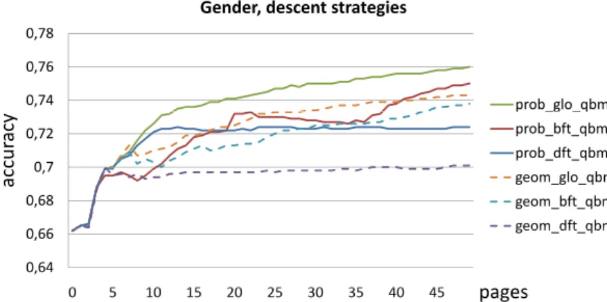
12.1 Alternative descent strategies . . . 207
12.2 Evaluation of descent strategies . . . 213
12.3 Conclusion . . . 215
13 Robust Anytime Stream Clustering 217 13.1 The LiarTree . . . 217
13.2 Experiments . . . 229
13.3 Conclusion . . . 235
14 Application: Using Modeling for Anytime Outlier Detection 237 14.1 Introduction . . . 237
14.2 Related work . . . 238
14.3 Detecting outliers in streaming data . . . 240
14.4 Experiments . . . 243
14.5 Conclusion . . . 250
15 MOA and CMM 251 15.1 The MOA Framework . . . 252
15.2 Evaluation Measures for Stream Clustering . . . 260
16 Future Work 263
IV
Summary and Outlook
265
V
Appendices
I
Bibliography III
Statement of Originality XLI
List of Publications XLIII
Data is collected and stored everywhere, be it images or audio files on private computers, customer data in traditional or electronic businesses, per-formance or control data in production sites, web traffic and click streams at internet providers, statistical data at government agencies, sensor mea-surements in scientific experimentation, surveillance data, etc. There are countless examples, and the amount of data is tremendous. Data mining is the process of finding useful and previously unknown patterns in data. In the examples listed above, data mining can be used for automated recommen-dation of audio files, business analysis and target marketing, or performance optimization and hazard warnings. While early mining algorithms only con-sidered static data sets, research and practice in data mining must nowadays deal with continuous, possible infinite streams of data, which are prevalent in most real world applications and scenarios.
Anytime algorithms constitute a special type of algorithm that is well suited to work on data streams. They inherit their name from their ability to provide a result after any amount of processing time. The amount of time available is not known to the algorithm in advance: anytime algorithms quickly compute an initial result and strive to improve it as long as time remains. When interrupted they deliver the best result obtained until that point in time.
In this thesis anytime classification is studied in depth for the Bayesian approach. New algorithmic solutions for anytime classification are devel-oped and evaluated in extensive experimentation. The first anytime stream clustering algorithm is proposed, and an application to anytime outlier de-tection is presented. In addition to the algorithmic contributions, new meta-approaches are described that significantly widen the area of applications for anytime algorithms. The solutions and results of this thesis contribute to the state of the art in anytime algorithms and stream data mining research.
Die rasante Entwicklung der Informationstechnologie hat zur Folge, dass in allen Bereichen der Gesellschaft und des t¨aglichen Lebens große Mengen an Daten erzeugt und gespeichert werden. Beispiele reichen von Multimedia-Daten auf privaten Computern bis hin zu Messdaten in wissenschaftlichen Experimenten. Data Mining beschreibt die Aufgabe, in solchen Daten neue und interessante Muster zu finden. Diese k¨onnen beispielsweise zur automa-tischen Empfehlung von Filmen genutzt werden oder helfen neue Zusam-menh¨ange aufzudecken und Prozesse zu verstehen. Seit Beginn der Data Mining Forschung w¨achst die Gr¨oße der zu verarbeitenden Datens¨atze. W¨ahrend Datens¨atze zun¨achst als statisch und vollst¨andig gegeben angenom-men wurden, generieren viele Anwendungen heute kontinuierliche und teil-weise unendliche Datenstr¨ome.
Anytime-Algorithmen stellen eine Klasse von Algorithmen dar, welche sich besonders gut zum Einsatz auf Datenstr¨omen eignet. Ihr Name r¨uhrt von ihrer Eigenschaft her, zu jeder Zeit ein Ergebnis liefern zu k¨onnen. Die zur Verf¨ugung stehende Zeit ist dem Algorithmus dabei nicht bekannt: er berechnet ein initiales Ergebnis und verbessert dieses solange zus¨atzliche Rechenzeit vorhanden ist. Wird der Algorithmus unterbrochen, so liefert er das beste Ergebnis zur¨uck, welches bis zu diesem Zeitpunkt erzielt wurde.
In dieser Dissertation werden neue Anytime-Verfahren f¨ur die Bayes Klassifikation entwickelt, intensiv untersucht und evaluiert. Der erste Anytime-Algorithmus zum Clustern von Datenstr¨omen wird vorgestellt und eine Anwendung f¨ur die Erkennung von Ausreißern wird diskutiert. Neben neuen Algorithmen werden zwei ¨ubergeordnete Verfahren entwickelt, die den Anwendungsbereich f¨ur Anytime-Algorithmen signifikant erweitern. Die in dieser Dissertation vorgestellten Ans¨atze und Resultate tragen zum Stand der Forschung im Bereich Anytime-Algorithmen und Data Mining auf Daten-str¨omen bei.
Introduction
The Need for Anytime Algorithms
The rapid development of computer and information technology fundamen-tally changed many processes in science, industry and daily life. Systems for collecting, storing and managing data evolved from primitive file processing systems to sophisticated and powerful database systems. The tremendous amounts of data soon exceeded the human ability of comprehension and thus called for advanced tools for analysis, compression and exploration. Knowledge discovery from data bases (KDD), or data mining, emerged as an interdisciplinary research field from the areas of data bases, machine learn-ing, statistics, visualization and other areas. Many mining algorithms were invented that helped reducing data, automatically classifying new objects based on historical data or extracting rules and correlations that exhibit novel patterns and useful knowledge.In early days of data mining research data sets were often considered static and given as a whole. This assumption allowed mining algorithms to perform random access on the data and to process objects multiple times during execution. With ever growing amounts of data the need for efficient processing yielded single pass algorithms and general solutions for fast ac-cess to large data sets were developed.
A data stream is a continuous, possibly endless sequence of data items that must be processed as they arrive. Many real world applications can be associated with data streams as large amounts of data must be processed
every day, hour, minute or even second. Examples include business/market data in companies, medical data in hospitals, statistical data in governmental institutions, experimental data in scientific laboratories, click streams in the world wide web, traffic/network data at web hosts or telecommunications companies, financial/stock market data in banking institutions, transaction/ customer profile data in e-commerce companies, etc.
Mining on data streams can basically perform the same tasks as mining on static data sets. Summarization or clustering are important tasks in stream mining, since they help to reduce the amount of data and can provide an overview of the data distribution. Other major tasks are streamclassification
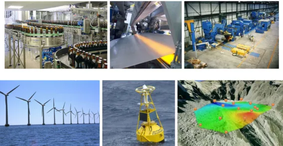
and outlier detection on data streams. Figure 1.1 shows real world examples of data stream applications where such mining tasks are crucial. Sorting items on a conveyor belt is an application for stream classification (cf. top left of Figure 1.1). In the example the bottles correspond to the data items and the classifier must sort out the broken or dirty bottles while usable bottles can pass. Similar applications are continuous quality checks in production sites such as surface inspection in paper, fabric or foil production (cf. top row of Figure 1.1, middle and right).
The first example in the second row of Figure 1.1 shows an application for both classification and outlier detection. The image shows an offshore wind farm and is associated with remote monitoring of machinery in general. In these applications measurements such as temperature, pressure or frequency spectra are taken at regular intervals and sent to a remote monitoring center, where the data is analyzed. The analysis can facilitate classification of the current status, detection of abnormalities or prediction of future measure-ments for hazard warnings. The center image shows a buoy of a tsunami warning system, the image right to it illustrates a network of sensors spread on a glacier in Switzerland. In both cases environmental parameters are measured and sent to base stations where these measurements constitute a stream of data objects. While classification and outlier detection has priority in both applications, generating models and distributions of the incoming data can be of interest for researchers and decision makers.
emergency professional decision full classifier pre classifier normal
Figure 1.1: Examples for real data streams.
The bottom part of Figure 1.1 illustrates the HealthNet project that has been conducted at RWTH Aachen University within the UMIC research clus-ter (cf. Chapclus-ter 8 for details). A central part in the HealthNet project is a body sensor network that measures vital functions of patients or elderly people. Those measurements are transferred to a mobile device for a first analysis and then partially forwarded to a central server depending on the results of the local analysis. Again the above mentioned tasks of classifying, detecting, predicting and modeling such patient data are useful and impor-tant.
Summarizing the review of data streams in real world scenarios it be-comes clear that basically everywhere where data is continuously measured, sent and analyzed, we find a potential application for stream data mining.
From the nature of a data stream and the properties of the system, on which the mining algorithm is executed, the following restrictions and con-sequential requirements emerge:
• endless stream – due to the fact that a data stream is possibly endless, the amount of data must be considered as infinite. As a consequence, algorithms are only allowed a single scan over the data. While some objects can be buffered to be processed again later on, nearly all items can be considered at most once. Moreover, the data must be processed in the order of its arrival; random access as in traditional data mining is missing in the streaming context.
• limited time – since data is continuously arriving, the time to process a single object is limited. Spending more time on an item by not process-ing other items (droppprocess-ing, samplprocess-ing) is prohibitive in many applica-tions such as sorting or outlier detection. Therefore the available time is mostly dictated by the actual or average time between two consecu-tive stream items. To this end the algorithms must provide fast access and cheap functions to process incoming objects online.
• limited memory – the limitation of physical memory and the infinite amount of data naturally yield the need for a compact representation of historical data using effective data structures. Storing all data objects is in most cases practically infeasible.
• evolving data distribution – maintaining an up to date model of the data distribution is crucial for many applications and algorithms. How-ever, in a data stream scenario the underlying model of the data dis-tribution often changes over time; concepts may shift or disappear and novel concepts can emerge. To focus on recent data, algorithms must provide ways to update their models and also forget or weigh down older data. Besides maintaining a valid model, the detection of changes in the data distribution is a new task that emerged in stream data min-ing.
• noisy data – noise in data streams corresponds to improper data tuples that can result from faulty sensor readings, for example. It is important for a mining algorithm to be robust against noise and offer appropriate ways of noise handling.
• varying data rates – the majority of data streams do not exhibit the same data rate over the entire time of their existence. On the contrary, many applications produce data at massively changing rates, for ex-ample due to daytime or seasonal changes in transaction data. Even rather stable data streams show varying data rates over time such as changes in conveyor belt speed in production. The varying data rates imply varying time allowances, which are in many cases unforeseeable. For some of the above aspects effective solutions have been proposed that are shared by many approaches. For limited time and limited space, established methods are available that are discussed in Chapter 3 along with common methods of dealing with evolving data distributions. Coping with single scan and missing random access is the core of any streaming algo-rithm. Also, the handling of noise is done in very individual ways (or even left out), since there is no clear definition of noise. Varying data rates and their implications are the focus in the remainder of this chapter.
The requirements for stream mining algorithms demand that items must be processed as they arrive. The available time for processing is naturally limited by the time between two consecutive items and may vary greatly in many applications. Referring back to the data stream applications from Figure 1.1 we take sensor networks as one example. Many sensor networks strive to reduce the amount of data that must be sent either to spare network bandwidth or energy resources, since sending data consumes much energy and often sensors are battery powered. Therefore, measurements are ag-gregated or only sent if they deviate significantly from the previous measure-ment. While this can yield unforeseeable inter-arrival times already for single sensors, it often results in data streams of massively changing data rates at base stations or monitoring centers. More moderate changes in stream rates can be expected at production sites and conveyor belt applications. However,
frequencies may differ as well on a daily, weekly or monthly basis. Finally, streams of business data or network traffic data exhibit high volatility for daytime or seasonal reasons.
As discussed previously, sampling or dropping of data items is prohibitive for many applications such as sorting or outlier detection. Since in varying data streams the duration of a burst or the number of objects that arrive within a certain time window is generally not bounded, simply buffering objects until the stream slows down is an option, neither. If the buffer size is exceeded, objects are lost. Moreover, buffering objects can largely delay the time of their processing and hence consecutive actions or reactions may not be initiated on time.
To process each item as it arrives traditional algorithms must base their computational model on the worst case assumption. More precisely, to be able to keep up even with the highest expected stream rate, the processing time for a single item must be strongly related to the corresponding small-est inter-arrival time. While parallel processing can speed up algorithms, it cannot break the dependency on the smallest time allowance. To finish the computation within a specific time budget, an algorithm can be restricted and tailored to the contracted budget. Clearly this yields large amounts of idle times, since the algorithm would finish his computation in the same time even if the available time is larger by orders of magnitude. While this is a drastic restriction for highly volatile streams, even for rather constant streams with smaller seasonal changes as in production sites, models must be built according to the minimal time allowance and, hence, the idle times add up and can become massive.
Optimally, an algorithm should be able to process an object in very short time and use any additional computation time to improve its outcome as long as permitted by the application. Consequently, idle times would be reduced or even avoided, the overall output of the algorithm would be improved, and the need to tailor algorithms to an expected or minimal time budget becomes obsolete. The idea of being able to provide a result regardless of the amount of available computation time lead to the development of anytime algorithms.
Definition 1.1 Anytime algorithm. For a given input an anytime algorithm can provide a first result after a very short initialization time and it uses addi-tional time to improve its result. The algorithm is interruptible after any time and will deliver the best result available at the point of interruption.
Anytime algorithms have first been discussed in the artificial intelligence community by Thomas Dean and Mark Boddy in [DB88] and have thereafter been an active field of research [Bod91, Zil96, GZ96]. Recent work includes an anytime A* algorithm [LGT03] and anytime algorithms for graph search [LFG+08]. Related concepts include anyspace [RC05, YWKMN09] and
any-cost algorithms [EM11].
Anytime algorithms differ from online algorithms and stream algorithms. Online algorithms refer to computing with incomplete information; the input is given one piece at a time [BEY98]. In addition to that, stream algorithms consider limited resources explicitly, for example a fixed maximal amount of time or memory. In contrast to anytime algorithms, neither of the two categories requires the algorithm to be interruptible at any time.
Not every application needs an anytime algorithm. In many applica-tions there may always be enough time to compute even the most detailed model. However, it is unquestioned that in many applications the available data largely increases in both size and complexity. This implies on the one hand that models become more complex, too, leading to higher computation times. On the other hand the increasing amount of data to process yields smaller time allowances per object. Multi-core processors and paralleliza-tion are not a one-fits-all soluparalleliza-tion to increasing complexity and decreasing time allowance. Large enterprises, especially web-scale endeavors, employ newest hardware and large scale server installations. While this may solve the case for some, others cannot afford giant hardware resources either due to economic reasons or contextual restrictions. Embedded systems, sensor networks, and mobile devices, for example, naturally own only very limited resources.
The anytime principle is applicable to many mining tasks and other algo-rithms. Classification is used as an example for the remainder of this section.
0,8 1 ur acy 0 4 0,6 acc 0 0,2 0,4 0 0.0 0.5 1.0 1.5 2.0 2.5 3.0 3.5 time
Figure 1.2: Anytime classification accuracy curve.
An anytime classifier can provide a first classification result for a given object after a short initialization. If it is not interrupted by the application, the algo-rithm continues processing the object to improve its classification decision; the accuracy of the result increases with the available computation time. Fig-ure 1.2 shows the curve of a typical evaluation result for an anytime classifier (if the algorithm works correctly): very small time allowances typically lead to medium classification accuracy, with greater time allowances the accuracy increases asymptotically towards its maximum.
The evaluation principle of anytime algorithms is somehow opposite to evaluating traditional algorithms. Traditional algorithms are often compared in terms of their efficiency, stating how many resources (most often time) they need to achieve a certain goal. This corresponds to the minimum prin-ciple, or principle of thrift, known from economy, which strives to reach a certain output with the least possible input. Anytime algorithms rather cor-respond to the maximum principle, or principle of yield, which strives to yield the highest possible output given a certain input. Evaluating an any-time classifier hence asks the question ”how accurate is the classifier for a given amount of time?”. Taking the varying time allowances into account, not only the single time accuracy value pairs are of interest, but also the accuracy increase between two different time allowances as well as the av-erage accuracy over a given distribution of time allowances. Details on these evaluation methods are provided in Chapter 4.
Anytime algorithms are obviously the best choice for data streams with varying data rates. Also on constant data streams, where every inter-arrival interval is always strictly the same, anytime algorithms can be beneficial and clearly outperform traditional budget algorithms. Consider the first
applica-tion from Figure 1.1, bottles on a conveyor belt in a brewery, for example. At some point the bottles pass a camera or the like, where features are extracted that are used in a classifier to decide whether the bottle must be sorted out or not. If the time between two bottles is known in advance, lets say 50 milliseconds, then a budget algorithm can be designed that delivers a classi-fication result within that budget of 50 milliseconds. If the budget would be higher the resulting accuracy of the classifier is likely to be better, because it has more time and can process a more detailed model. However, the budget algorithm spends the same amount of time on each item, i.e. on each bottle. In reality there are bottles for which the decision is very clear even after a very short time, as in the case of a bottle that is broken or clearly wasted. At this point an anytime algorithm can be used to not spend any more time on these certain decisions and to take advantage of the gained extra time for other items, where a clear decision requires a more detailed model. This way, the overall performance of an anytime algorithm (the accuracy in this example) exceeds that of a traditional budget algorithm even on a constant data stream. In Chapter 9 different approaches to harness the strength of anytime algorithms on constant streams are proposed along with details and experimental analyses.
The abundance of data streams and applications and the superiority and usefulness of anytime algorithms on both varying and constant streams moti-vated the research that is presented in this thesis. Novel methods for anytime classification are developed and the first anytime algorithm for clustering on data streams is proposed. The outline of the thesis is provided in the next section.
1.1
Thesis structure
This thesis consist of five parts: I Introduction, II Anytime Stream Classifi-cation, III Anytime Stream Clustering, IV Summary and Outlook, and the appendices in Part V.
The introduction contains the motivation, the background, and the main concepts for stream data mining and anytime algorithms. We have seen that data mining algorithms are important in many applications and that streams are ubiquitous in all areas of our daily life. The special requirements of stream mining algorithms were discussed and anytime algorithms resulted as most flexible and the best choice for both varying and constant streams. In the remainder of the introduction the KDD process and general mining tasks are reviewed in Chapter 2 and specific tools and algorithms for stream data mining are discussed in Chapter 3.
In part II the focus is on anytime classification on data streams. Novel approaches for anytime stream classification are presented in Chapters 4 – 7 and an application of the proposed anytime classifier is shown in Chapter 8. Two concepts for using anytime algorithms on constant streams are proposed in Chapter 9, future work in the area of anytime stream classification is dis-cussed in Chapter 10.
In Part III anytime clustering on data streams is introduced. Novel ap-proaches for anytime stream clustering are proposed in Chapters 11 – 13, an application of the proposed technique for anytime outlier detection is shown in Chapter 14. Chapter 15 deals with the evaluation of stream clustering algorithms presenting a software framework for stream mining and a novel concept for the evaluation of clusterings on evolving data streams. Future work in the area of anytime stream clustering is discussed in Chapter 16.
Part IV summarizes the thesis and provides a general outlook for future research in the area of anytime algorithms and stream data mining.
The appendices in part V provide the bibliographic references as well as additional information on the author and his contributions in this thesis in the form of a statement of originality, a list of publications, and a curriculum vitae.
Knowledge Discovery from Data
This chapter contains background information on the KDD process and in-troductions to basic data mining tasks, algorithms and challenges. Readers familiar with data mining may want to skip this chapter and proceed with Chapter 3, where more specific techniques for stream data mining are dis-cussed.2.1
The KDD process and data mining tasks
Knowledge discovery from data is an iterative process that contains multiple steps which are illustrated in Figure 2.1. Before the actual data mining is performed the desired data must be extracted and validated. This requires that a thorough preprocessing precedes the mining step.
Data cleaning refers to the removal of noise and inconsistencies in the raw data. These can be missing values or values that are outside the al-lowed range and can occur among others due to faulty measurements, hu-man errors during data acquisition or deliberate hu-manipulation. Integration
of data refers to the combination of data from multiple sources, which can be different companies, different users or different time spans. Challenges in data integration include differences in naming conventions, missing at-tributes or a different schema in general. Data selection is the restriction to relevant data; only those tuples and attributes are retrieved that are
Data bases Data Warehouse Preprocessed Data Patterns Knowledge Cleaning and Integration Selection and Transformation Data Mining Evaluation and Presentation
Figure 2.1: From data to knowledge: Illustration of the KDD process as de-scribed in [HK01] and others.
esting and necessary for the impending task. Transformation is the last step in the preprocessing where the data is altered to meet the requirements of the following mining algorithm. Normalization or unification of value ranges can be performed in this step as well as aggregation, binarization or other transformations.
The preprocessing is followed by the actualdata miningstep, where algo-rithms are applied that extract patterns from the data. These pattern are for example groups of data objects described by representatives, models or rules that are found by the algorithm. While representatives can be used for data reduction, models can identify abnormalobjects that strongly deviate from the model, and rules can be employed to classify previously unknown data objects. Examples for data mining tasks are provided below.
The evaluation step is as crucial as the mining step and is often consid-ered as a part of the data mining algorithm itself. The goal in this step is the identification of the truly interesting patterns; evaluation is similar to a filter or pruning step that reduces the amount of found patterns to those that are most important according to some interestingness measure. Presentation of the found patterns is most often done by visualization and knowledge repre-sentation techniques. It supports the user in exploring and interpreting the results and can provide hints for further mining and analysis steps. Finally, the found patterns can be integrated into the data repositories and used in further iterations of the KDD process.
Data mining is a central step in the KDD process. In the following the most recognized mining tasks are introduced along with brief explanations and examples. Since two tasks, namely classification (Part II) and clustering (Part III), constitute core parts of this thesis, a formal definition is provided for these as well. In the remainder of this thesis an object or point is re-ferred to as a d-dimensional tuple or vector, where each dimension is called an attribute or a feature of the object. In general objects can be from an arbi-trary metric space; if not mentioned differently, thed-dimensional Euclidean vector space Rd is assumed as the domain for all objects and the Euclidean
distance between two pointsxandyis denoted as d(x, y).
Classification. Classification describes the process of assigning a previ-ously unknown object to a category orclassbased on its features. To this end a classifier builds a so called model from the given training data in the train-ing phase and uses this model to process new objects in the testtrain-ing phase. Definition 2.1 Classifier. For an input space Q and a set of class labels L ={l1, . . . , l|L|} a classifier trains a set of internal model parametersΘbased
on a set of training data T ⊆ Q × L (and possibly external parameters). A classifierC is associated with a functionfC(Θ, q)that assigns an object q∈ Qto a class label based on its parametersΘ.
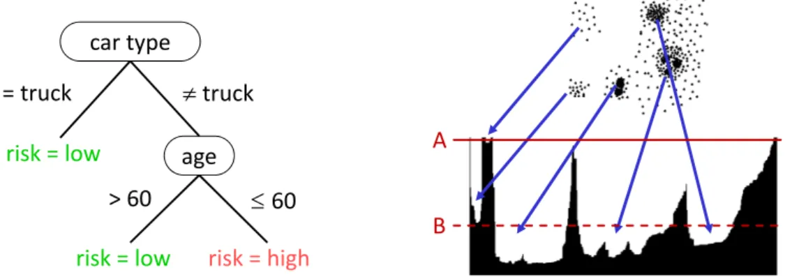
One well known family of classifiers are decision trees [BFOS84, Qui93], the left part of Figure 2.2 illustrates an example. A node of a decision tree is associated with an attribute, the outgoing branches correspond to an at-tribute value. In the example the risk for accidents is determined based on the two attributes ”car type” and ”age”, possibly useful for an insurance com-pany. While the root node branches according to a match in the categorical attribute ”car type”, the second node applies a threshold on the continuous attribute ”age”. A thirty year old person driving a sports car would be as-signed a high risk according to this decision tree. The tree is the actual model of the classifier that is learned in the training phase. A way to improve the accuracy of a classification method is to build an ensemble of several clas-sifiers. For a decision tree one could for example build several trees from
A B = truck > 60 60 risk = high risk = low truck risk = low car type age
Figure 2.2: Left: decision tree classifier. Right: a result of the OPTICS clus-tering algorithm. (Examples taken form lecture slides corresp. to [HK01]). different random samples of the training data. The classification decision can then be obtained by a majority vote on the results of all trained trees.
Prediction and regression are similar to classification. In regression the output of the algorithm is not from a limited set of class labels, but can be a numerical value. Prediction refers to finding the most probable future value based on a series of previous values or value tuples. Classification is also termed supervised learning, since the class labels of the training set are known in advance.
Clustering. Clustering refers to grouping of data objects, such that the objects within a group exhibit a high similarity and objects from different groups are dissimilar. Since in contrast to classification the labels of the objects are not known, clustering is also called unsupervised learning. A clustering algorithm takes a data set as an input and returns a set of groups called clusters.
Definition 2.2 Clustering. Given a data setO ⊆ Qfrom an input spaceQa clusteringC ={C1, . . . , Ck}is a set of groupsCi called clusters. Each clusterCi
is a non-empty subset of objects fromO: Ci ⊆ O with|Ci|>1,∀i= 1. . . k.
The most popular clustering methods are so calledk-center clustering al-gorithms including k-means [Llo57], k-medoids [KR90] and their variants. They take the number of clustersk as an input parameter and try to find k representative centers such that a given objective is minimized. The
objec-tive is most often a variant of the sum over all squared distances from the objects to their closest representative. Since finding the optimal solution to this problem is NP-hard, clustering algorithms heuristically search a local op-timum as their solution. Besides k-center clustering algorithms many other approaches have been proposed such as density-based clustering methods. One example is the OPTICS algorithm [ABKS99], the right part of Figure 2.2 shows a result of the algorithm. Each valley in the plot corresponds to a cluster in the data set, a horizontal line corresponds to a threshold value for the minimal cluster density. If A is chosen as a threshold, the two small groups on the left side are returned as two clusters and the remaining points are considered as a third cluster. Choosing B as a threshold results in three clusters as well (dense areas in the right group of points), but the objects on the left and the scattered points on the right are not included in a cluster.
Outlier analysis. Objects that deviate significantly from the rest of the data set are called outliers. There is no clear definition and, consequently, different approaches can find different outliers in the same data set. In the OPTICS algorithm described above, the objects that were not included in any cluster are considered outliers (cf. threshold B), since their region of the data space does not exhibit a sufficient density. Other algorithms determine outliers using distance-based [KNT00], angle-based [KSZ08] or statistical approaches [BL94].
Frequent patterns/Association rules. Market basket analysis is a com-mon application for association rule mining or frequent pattern mining where sets of items are searched that frequently occur together. In the example they correspond to products that are often bought together. The goal is to find rules of the form ”If customer X buys milk and bread he will also buy cheese (with a certain probability)”. Technically, an association rule is of the form ”head→body (support, confidence)” where body follows as a con-sequence from head, support is the number of times that the pattern was observed and confidence is the relative frequency of head compared to the support of the rule. Efficient methods to compute all association rules for given support and confidence values have been proposed in the literature [AIS93, AS94, HPY00].
Concepts description (characterization, generalization, discrimina-tion). Characterization is a summarization of the general characteristics or features of a group of objects such as age, job and income of people that regularly go on a cruise. Generalization is an automated process that groups objects based on their characteristics. An example is attribute oriented induc-tion [CCH91]. Discriminainduc-tion finds characteristics that separate two groups of objects (contrasting classes), for example those customers that frequently buy product X and those that rarely buy it.
In this thesis new methods are mainly developed in the areas of classifica-tion and clustering. A more detailed review of existing approaches in those areas can be found in Sections 2.2 and 3.2 for classification and Sections 2.3 and 3.3 for clustering, where the corresponding section in Chapter 3 con-tains the stream specific methods. As an application of a proposed technique outlier detection is discussed in Chapter 14. The corresponding related work on outlier detection is discussed in that chapter. For a more detailed general introduction to data mining please refer to [HK06]. In the following section challenges in data mining are presented that arise due to certain properties of the data or requirements of the application. A broader introduction to those topics can be found in [KHY+09].
2.1.1
Challenges in data mining
Many mining algorithms rely on a notion of similarity between objects or representatives: clustering algorithms group objects based on similarity, a classification algorithm can assign labels based on similarities, etc. Efficient mining algorithms therefore often require methods that allow for fast simi-larity search in large data sets. Simisimi-larity is most often assessed by the use of a distance measure such as the Euclidean distance. To speed up similarity search a plenitude of methods and data structures have been proposed that facilitate fast access. In hierarchical index structures directory information is organized in a tree structure. When executing a similarity search query, these methods try to access only very small parts of the data by steering the search using the tree structure. Examples for index structures include the
popular B-trees [Com79], R-trees [Gut84, BKSS90], M-trees [CPZ97] and KD-trees [Ben75], as well as specialized methods such as the RI-tree [KPS00] or the TS-tree [AKAS08]. Besides hierarchical index structures many other approaches for fast similarity search have been proposed including bitmap indexes [CI98] or hashing techniques [DIIM04].
A major challenge are very high dimensional spaces. In high dimensional spaces distances lose their expressive power, since all distances tend to be similar. This problem is known as the curse of dimensionality, which af-fects similarity search and hence also mining algorithms. Specialized index structures for high dimensional spaces have been proposed such as X-trees [BKK96] and TV-trees [LJF94]. The VA-file [WSB98] constitutes a filter-and-refine approach that first computes a set of candidates using a lower dimen-sional representation of the data and refines the set in the full space in a second step. Other lines of research focus on approximate similarity search in high dimensional spaces [HS05] or try to avoid using distances and de-termine the association between objects by the means of shared-neighbor information [Hou08, HKK+10]. To circumvent the problems resulting from
the similarity of distances in high dimensional spaces, subspace clustering al-gorithms search for solutions in different subsets of the attributes [AGGR98, APW+99, AY00, CFZ99, AKMS08]. Since the number of different subspaces
is exponential in the dimensionality of the original space, these algorithm are faced with a huge combinatorial complexity.
Time poses different challenges on data mining algorithms, ranging from volatile data bases to dynamic and endless data streams. Time aspects, es-pecially requirements and solutions for stream data mining, have been dis-cussed in Chapter 1 and are the main topic throughout the thesis. A different notion of time in data sets and mining algorithms is introduced by time series data. Time series denote sequences of values over time which are available entirely before processing them in an algorithm. Hence, in contrast to dy-namic data streams, time series constitute a static type of data. Mining on time series data includes searching for reoccurring or unusual patterns to discover trends or conspicuous behavior [AS95, HDY99, KGI+11].
A further challenge lies in the structure of the data. New technologies and new phenomena yielded complex data types such as multimedia data [Sub98], text data [SM84], graph data as in social networks [New03], gene sequences and molecular structures [BB01] and other domain-specific data types. For multimedia data even a single image is often represented by a large number of features describing color, texture or salient points in the image [HLZ02]. Specialized distance measures have been proposed that are claimed to reflect the human perception of similarity [SK97, RTG00]. Mining video data has many applications such as video copy detection, but remains a major challenge in data mining research [CZ06, AKS10]. Other complex data types pose their own difficulties but also offer new questions and tasks. From there many new directions in data mining research emerged such as graph mining or text and semantic mining [WM03, WIZD04, WF94].
Although pattern evaluation has always been a step in the KDD process (cf. Figure 2.1), it got new attention with the advent of complex methods and data types. One example is the exploration of subspace clustering results [MAK+08], where the number of found clusters can sometimes be larger
than the actual size of the data set. This is due to the exponential number of different subspaces in which clusters can be found. More precisely, since generally objects can be in more than one cluster, the found clusters often largely overlap with respect to the contained objects. To this end measures for redundancy and interestingness have been proposed and included into algorithms either during the cluster search or as a post processing component [MAG+09a, AKMS08]. Similar issues and solutions apply for other mining
tasks such as frequent item set mining [BEX02].
Finally there is a list of other issues that reveal limitations of mining al-gorithms and open up new research directions. Examples are privacy and security issues that either restrict the access to data or the validity of re-sults [CM96, VBF+04]. Parallel and distributed data mining algorithms try
to meet the requirements of growing data repositories by efficient strategies to share data and computation across large networks of servers and clients [PCY95, AS96, PHBB09]. The popularity of sensor networks, global posi-tioning systems (GPS), cellular phones, other mobile devices and RFID
tech-nology yielded vast amounts of moving object data that calls for effective methods for analysis and knowledge extraction [DeC97, PZZ+07, CBB08].
The internet can be seen as a synonym for many of the challenges men-tioned above. It represents graph data, text data and heterogeneous data, poses privacy and security issues, is massively distributed and parallel and has obviously a tremendous size.
2.2
Classification
In this section the main concepts and approaches proposed for classification on static data sets are reviewed. Stream classification algorithms are dis-cussed in Section 3.2. Before going into detail on the individual approaches a more formal description of a classifier based on Definition 2.1 is provided. Given an input space Q of dimensionality d and a set of labels L =
{l1, . . . , l|L|}, the extended input space of labeled objects is denoted asQ+ =
Q × L. The power setP(Q) of Qcontains all possible subsets ofQ, P(Q+)
analogously for Q+. The training set for a classifier can then be written as
T ∈ P(Q+) and a test object for classification as q ∈ Q. T
l = {o ∈ T |o =
(o1, . . . , od, l)}denotes the set of objects fromT with labell.
Any classifier C can be described by a modelM which is in turn defined as set of parameters M = {ψ1, . . . , ψ|M|}. The domains of the parameters
are denoted as Dom(ψ), and Dom(M) := Dom(ψ1)× . . .× Dom(ψ|M|) is
the cross product of all parameter domains. A configuration or instantiation of the model M is a set of values Θ ∈ Dom(M) for its model parameters:
Θ = (θ1, . . . , θ|M|)withθi ∈Dom(ψi) ∀i= 1. . .|M|.
To build a classifier, any approach must first select a model and second choose, or optimize, its parameter values. To this end it can consider the training set T and possibly a set of external parameters Φ = {φ1, . . . , φ|Φ|}.
Similar to the above the parameter domains are denoted as Dom(φ) and Dom(Φ) := Dom(φ1)×. . .×Dom(φ|Φ|). A set of external parameter values
is called Ξ = {ξ1, . . . , ξ|Ξ|} with ξj ∈Dom(φj) ∀j = 1. . .|Φ|. The selected
model is
where η : Dom(Φ)×P(Q) 7→ M is a model selection function that selects a modelM from the model space Mbased on the training set and external parameters. The values for the model parameters are chosen in a second step as
Θ =πC(M,T) (2.2)
whereπ :M ×P(Q)7→Dom(M)is a parameter optimization that is based on the selected model and the training set andDom(M) = S
M∈MDom(M).
Finally, the label of a test objectq∈ Qis determined by the classifier as
l=fC(Θ, q) (2.3)
using a decision functionfC :Dom(M)× Q 7→ Lthat assigns a label based on
the model parametersΘ. Thus, without loss of generality, the general task of a classifierC is to determine
l =fC(πC(ηC(Ξ,T),T), q). (2.4)
Finding the set of parameter values Θ = πC(ηC(Ξ,T),T) is usually
re-ferred to as thetrainingof a classifier, also calledlearningorsupervised learn-ing, since the class labels of the training set are known. Applying the decision function on a set of test objects is often termedtestingof a classifier.
The performance of a classifier is mostly measured in terms of its classifi-cation errorerr or classification accuracyacc= 1−err corresponding to the proportion of correctly classified objects. Examples for further analysis and performance measures like the confusion matrix, sensitivity, precision or the ROC curve can be found in [HK06]. To assess the performance of a classi-fier on some given data setD ∈ P(Q+), an m-fold cross validation splits D
intom equally large parts (folds) and uses successively one part for testing and the remaining parts for training. A different approach called bootstrap-ping uses m subsets Di of size |Di| = |D| sampled randomly from D with
replacement and usesDi for training andD\Di for testing fori= 1. . . m.
For the plethora of classification algorithms, different approaches have been suggested to categorize the proposed methods [HK01]. One approach
distinguishes lazy learners and eager learners, while the latter category is larger by far. Lazy learners spend little or no computation time on model selection and parameter optimization, but defer the work to the decision phase. Eager learners on the other hand exhibit more time consuming train-ing procedures and are in turn often more efficient in the decision phase. A different categorization separates generative and discriminative methods. The objective in training generative classifiers is to build a model that best describes the classes L as given by T, as if the model was generated by T. This is opposed to discriminative methods, which seek to best separate, or
discriminate, the different classes. Neither of these categorizations is fol-lowed here, but the terminology is referred to when describing the single methods. Among the presented classification approaches Bayesian classifi-cation is described in more detail, since it will be heavily used throughout the thesis. Support vector machines (SVM) and decision trees receive more attention that the remaining approaches, since both relate to parts of the methods presented in Part II. For SVMs a simple transformation to Gaus-sian mixture models is discussed and decision trees connect to the proposed methods by constituting a hierarchical approach.
Bayesian classification
Bayesian classification constitutes a statistical approach in which an object q∈ Qis assigned to a class labell∈ Lbased on membership probabilities. It is based on the Bayes theorem and one of the most frequently used methods for classification. The Bayes theorem for two events AandB is
P(A|B)P(B) = P(B|A)P(A), (2.5) where P(A) is the prior or a priori probability of A and P(A|B) is the pos-terior probability of A conditioned on B, also called the conditional prob-ability of A given B. In the context of a classifier, given a set of labels
L = {l1, . . . , l|L|} and an object o ∈ Q, P(li) and P(o) are the prior
prob-abilities for the labels and the object, respectively. P(li|o) is the posterior
prob-ability of o given label li. Using Equation 2.5 the Bayes classifier assigns to
an objectothe labelˆlthat yields the maximal posterior probability:
ˆl=f
Bayes(Θ, o) = arg max
l∈L {P(l|o)}= arg maxl∈L P(o|l)P(l) P(o) (2.6)
The probabilities on the right hand side of Equation 2.6 can be estimated fromT as follows. The class priors are estimated as the relative frequency of the labels inT:
P(l) = |{o∈ T |o= (o1, . . . , od, lo)∧lo =l}|/|T | (2.7)
The prior for the object is computed as P(o) =X
l∈L
P(o|l)P(l). (2.8)
However, as in the computation of ˆl the object o is not varied in the de-cision set {P(l|o)}, the term P(o) can be left out in equation 2.6, since it merely normalizes the probabilities but does not affect the decision (simul-taneous classification of several objects is discussed in Chapter 9). The way of estimating the class conditional probabilityP(o|l) defines different kinds of Bayesian classifiers. The approach known as na¨ıve Bayes assumes class conditional independence of all dimensions in Q, which allows to calculate the posterior probability foro as
P(o|l) =
d
Y
i=1
P(oi|l). (2.9)
The class conditional probabilitiesP(oi|l)for the single dimensions can again
be easily computed fromT by counting. EstimatingP(oi|l)requires different
approaches for categorical and continuous attributes.
For a categorical attribute Ai with possible valuesai1, . . . , aiu the
precomputed for every possible valueaij as
P(aij|l) =|{o ∈ T |o= (o1, . . . , od, lo)∧lo =l∧oi =aij}|/|Tl| (2.10)
Dropping the assumption of the na¨ıve Bayes allows to introduce dependen-cies between the attributes by defining the probability of attributeA having valueaiconditioned on attributeBhaving valuebj. For categorical attributes
the dependencies and the resulting probability distributions can be described by Bayesian networks, also termed belief networks or Bayesian belief net-works. A Bayesian networkB =hG,Θiis defined by a directed acyclic graph G and a set of parameter values Θ. G = (V, E) contains one vertex for each attribute and one vertex for L. An edge (v1, v2) ∈ E signifies that v2
is conditionally dependent on v1; there are exactly d edges in the Bayesian
network for the na¨ıve Bayes, one from L to each dimension (cf. Figure 2.3 left). For a vertex v ∈ V, let pa(v) denote the parents of v in G. Then the joint probability from Equation 2.9 for a Bayesian network classifier is
P(o|l) =
d
Y
i=1
P(oi|l,{oj|vj ∈pa(vi)}). (2.11)
ΘinBcomprises conditional probability tables that store a probability per attributevi for each combination of values fromvi,pa(vi)andL. Considering
the example in the right part of Figure 2.3 lets assume|L|= 4and |Ai|= 10
∀i= 1. . . d, then each attribute can have ten different values. This yields
|Θ|= 4 |{z} P(l) + 4·102 | {z } A1 + 4·10·5 | {z } A2,...,A6 + 4·103 | {z } A7 = 4604 (2.12) A1 A2 A3 A4 A5 A6 A7 L A1 A2 A3 A4 A5 A6 A7 L
Figure 2.3: Examples for Bayesian networks for the na¨ıve Bayes (left) and with additional dependencies (right).
which is opposed to |Θ| = 4 + 4·10·7 = 284 for the na¨ıve Bayes on the same example (cf. Figure 2.3 left). Besides higher space demands, the large number of parameters can frequently lead tozeroprobabilities, since certain value combinations do not occur in T. These zero probabilities can cancel the effect of all other posterior probabilities; if in the above example six attributes would yield a high probability, a zero probability in the seventh attribute would spoil the output. To avoid this, a Laplace correction can be applied that initially sets each count in the probability tables to one and takes this into consideration during the normalization.
The model selectionη(cf. Equation 2.1) for a Bayesian network classifier refers to the determination of the network topology (defining the edges in G). Proposed solutions are for example based on maximal correlation coeffi-cients [Edw00, SS05] or use hill climbing methods to iteratively add the most promising edges [KP02]. The parameter optimizationπ(cf. Equation 2.2) for Bayesian networks as introduced above can simply compute the probabilities in a generative way fromT (with or without Laplace correction) or can itera-tively perform cross validation onT to find parameter values that lead to the best discrimination of the classes inL. For Bayesian networks with hidden variables (not discussed in this thesis) there is an abundance of literature for network inference, introductions and examples can be found [RN95] and [Jen96].
For continuous attributes, the probabilities P(o|l) and P(o) in Equation 2.6 are substituted by density estimation functions denoted asp(o|l)andp(o). Usually the class conditional density p(oi|l) for a given object in dimension
i is computed using a parameterized density function g(oi,Θl) assuming a
certain distribution of the attribute values. The parameter valuesΘl for the
distributions of labell are derived fromT. The most popular example is the Gaussian distribution or normal distribution.
Definition 2.3 The Gaussian distribution N(µi,Σi) for a random variable X
with mean valueµand varianceσ2 is described by the probability density
func-tion
g(x, µ, σ) = √ 1
2πσ2e
−(x−µ)2
For a set{X1, . . . Xd}ofdrandom variables the joint probability distribution is
g(~x, ~µ,Σ) = 1 (2π)d2p|Σ|
e−12(~x−~µ)Σ
−1(~x−~µ)T
where~x∈Rdis ad-dimensional vector,~µ= (µ
1, . . . , µd)is the vector containing
the mean values ofX1, . . . Xd,Σis the corresponding covariance matrix,|Σ|its
determinant andΣ−1 its inverse.
For convenience g(x, µ,Σ) is used instead of g(~x, ~µ,Σ) for the d-dimen-sional case in the following. The joint probability distribution for continuous attributes naturally includes dependencies between all attributes via the co-variance matrix Σ. For the na¨ıve Bayes using Gaussian distributions, the covariance matrix constitutes a diagonal matrixΣ =diag(σ2
1, . . . , σd2)and the
posterior probability for an objecto simplifies to
P(o|l) =g(o, µ,Σ) = 1 (2π)d2 Qd i=1σi e− 1 2 Pd i=1 (oi−µi)2 σi2 (2.13)
Using a single Gaussian distribution to describe a set of objects is also called a unimodal model. A more flexible density estimation function is given if several Gaussian distributions are combined.
Definition 2.4 A Gaussian mixture model (GMM) with k components is a weighted combination of k Gaussian distributions with parameters (µi,Σi),
i= 1. . . k and is defined by the probability density function
gGM M(x,Θ) = k
X
i=1
wi·g(x, µi,Σi)
whereΘ ={µ1, . . . , µk,Σ1, . . . ,Σkw1, . . . , wk}is the set of all parameter values.
wi is the weight of thei-th Gaussian subject toPki=1wi = 1.
Besides unimodal models and mixtures of Gaussian, kernel density esti-mators constitute the most detailed model for density estimation based on training data. Kernel density estimation is detailed in Chapter 4, where ker-nels are employed in a novel anytime classification approach.
The model selection ηfor a Bayes classifier on continuous attributes can hence be viewed as selecting the type of density function, for example the number and type (na¨ıve or not) of Gaussians. The parameter optimizationπ can again determineΘfromT in a generative way by using the EM clustering algorithm (cf. Chapter 6) or in a discriminative way by using max margin optimization for example (cf. Chapter 7). A more detailed introduction to Bayesian classification as well as further references can be found in [DHS01].
Support vector machines
Support vector machines (SVM) constitute discriminative classifiers that seek to find decision boundaries, calledseparating hyperplanes, which best sepa-rate the objects from different labels. A binary SVM considers objects from two different classes denoted as +1 and −1 (l ∈ {+1,−1}). The decision function of a binary SVM is fSV M(Θ, q) =sign s X i=1 liαiK(xi, q)−b ! , (2.14)
where Θ = {(xi, αi)|i = 1. . . s} ∪ {b, K(·,·)} stores the bias b, the Kernel
K(·,·), the support vectors xi ∈ T and their weight αi. s is the number of
support vectors, li ∈ {+1,−1} is the label of xi and examples for kernels
K(·,·)are
polynomial kernel of degreeh: K(xi, xj) = (xi·xj+ 1)h
radial basis function (RBF) kernel: K(xi, xj) = e−γkxi−xjk
2
sigmoid kernel: K(xi, xj) = tanh(κxi·xj−δ)
The training of an SVM determines the weights αi for all objects oi ∈
T. Those objects with corresponding αi > 0 are used as support vectors
and are included in Θ. The actual training involves solving a constrained quadratic optimization problem, introductions and details to SVM can be found in [Vap95, Vap98, Bur98, Pla98].
In the case of |L| > 2 multiple binary SVMs are combined. SVM classi-fiers for |L| > 2can for example train |L| binary SVMs, each separating the objects from one label against all other objects, or quadratically many binary SVMs, one for each pair of labels. The final decision can then be reached by a majority voting or interpreting the outputs of the single SVMs as probabil-ities.
On a side note, there is a simple transformation between an SVM using RBF Kernels and a Bayes classifier using Gaussian mixture models with equal variance σ for each Gaussian and each dimension, which yields the exact same decision boundaries for both classifiers [DHN10]. Using the notation from Equation 2.13 the transformation is
xi = µi (2.15) αi = P(li)·wi· 1 (2π)d2σd (2.16) γi = 1 2σ2 (2.17)
Transforming an SVM into GMMs, the bias bcan be sufficiently well approx-imated by an additional Gaussian with arbitrary mean, very high variance and weightwproportional tob.
Decision tree classifier
An example of a simple binary decision tree was given in Figure 2.2, where the risk of an accident was determined based on the car type and the age of the driver. Generally, decision trees are not restricted to binary nodes but are allowed higher branching factors. The binary case is introduced below; the general case naturally follows from the description.
Definition 2.5 A decision tree node ν = (Ai, aij, p1, p2) stores a splitting
at-tribute Ai, a split value aij and two pointers p1 and p2 to the left and right
subtree. A Leaf node ν is associated with a set of training objects T|ν and an
For categorical attributes, aij splits T|ν into the two sets T|ν1 = {o|oi = aij}
and T|ν2 = {o|oi 6= aij}, for continuous attributes the two resulting sets are
T|ν1 = {o|oi < aij} and T|ν2 = {o|oi ≥ aij}. For higher branching factors,
additional values for the same attribute are stored inν as well as additional pointers to the corresponding subtrees.
The training of a decision tree is often referred to as decision tree induc-tion. Popular algorithms for decision tree induction are ID3 [Qui86], C4.5 [Qui93] and CART [BFOS84], which all follow a greedy top down approach to partition T recursively into smaller subsets. The algorithms seek to find the best split point, which is the best attribute Ai and attribute value aij,
for the current node ν with respect to some objective function. A popular objective, which is also used in ID3, is the information gain
IG(ν) =Ent(ν)− 2 X u=1 |T|νu| |T|ν| Ent(νu), (2.18)
whereEnt(ν)is the entropy of nodeν defined as
Ent(ν) =−X l∈L |Tl|ν| |T|ν| log |T l|ν| |T|ν| . (2.19)
Tl|ν extends the notation ofT|ν toTl. For higher branching factors the sum in
Equation 2.18 considers all subtrees. Since this yields a bias towards nodes with a larger fanout, other methods such as C4.5 use the gain ratio as their objective, which overcomes the bias by normalizing the information gain with the potential information for the split [HK06]. The induction termi-nates if for example either all objects inT|ν have the same label or the same
attribute values. There is a vast amount of literature on scaling decision tree induction to large data bases or improving decision trees, which is beyond the scope of this thesis.
During classification a query objectq ∈ Q follows the path from the root of the decision tree to a leaf νˆ according to its attribute values. The basic version of a decision tree then assigns a label based on a majority voting on
T|νˆ. Advanced versions associate distributions with the leaves of the tree and
Nearest neighbor classification
The nearest neighbor classifier (NN) [Das90, Sei09] is a simple classifier that belongs to the category of lazy learners. The idea is to assign to an object q ∈ Q the label ˆl ∈ L of the closest object o ∈ T with respect to a given distance functiondist(·,·)∈Ξ:
fN N(Θ, q) = ˆl ⇔ oˆ= (ˆo1, . . . ,oˆd,ˆl)∧oˆ= arg min
o∈T {dist(o, q)}
Here, the training set forms the parameters: Θ = T. Ties can be broken assuming a canonical ordering of the labels. Variants of the nearest neighbor classifier usek > 1objects, wherek ∈ Ξis an external parameter. The deci-sion based on thekresulting labels can be done using simple majority voting, weighting the frequencies with the class priors or weighting the influence of each object bydist(o, q)−1.
Ensemble classifiers
Ensemble methods combine several classifiers and arrive at a decision based on the combined outputs. As an example, classifiers of different kinds can be trained onT and the label l ∈ L for an objectq ∈ Qis determined via ma-jority voting. Bagging(bootstrapaggregation) [Bre96] is a popular ensemble method that trainskclassifiers (usually of the same type) onkdifferent boot-strap samples from T. Another popular method is Boosting [FS97], which weights the results of the single classifiers with respect to their performance on T. Moreover, in boosting the objects are weighted during training and the k classifiers are trained successively giving misclassified objects higher weights in subsequent trainings such that more attention is paid to them.
Neural networks
Neural networks are well known and very well researched. For a neural net-work classifier one must select a netnet-work topology and the type of neurons in a first step and learn or optimize the parameters of the network in a second
step. A frequently used training method for neural networks is backpropa-gation [RHW86, HB87, Jac88]. Using RBF-style neurons in a neural network yields the same decision hyperplane as an SVM with RBF kernels [HK06].
Besides the discussed classification algorithms there is a number of ad-ditional approaches including case-based reasoning and genetic algorithm as well as rough set and fuzzy set approaches; Please refer to [HK06] for a broader introduction. Each classification paradigm has its strengths and weaknesses. Bayesian classifiers are for example said to be less prone to overfitting since the employed probability distribution functions can provide an effective way of generalization. Clearly, there is no single solution that outperforms all other approaches on all domains and settings. Finding the best classifier for an actual application involves tuning and testing of various methods and is usually not addressed in the classification literature.
2.3
Clustering
Clustering tries to find groups of data, such that objects exhibit a high simi-larity within the groups and a low simisimi-larity between the groups (cf. Section 2.1). Research on clustering algorithms looks back at a long history. Since clustering is useful for many applications, approaches have been developed in different areas and from different perspectives. In this section the most prominent and frequently used clustering algorithms are reviewed.
The nature of clustering algorithms is often more heuristic compared to classification algorithms and their description appears therefore sometimes less formal. This holds true in a similar extent when it comes to the evalua-tion of clusterings that were found by an algorithm. A ground truth is hardly ever available; and even if, heuristics are needed to assess the quality of a found clustering. A wealth of measures can be found in the literature, some of which rely on a given ground truth clustering for comparison while other don’t. The measures employed in Part III are commonly used and will be introduced where needed. The matter of clustering evaluation on evolving data streams is discussed in Chapter 15.
Definition 2.2 defines a clustering C = {C1, . . . , Ck} as a set of groups
Ci, each of which is a non-empty subset of objects from a given data set O.
This general definition allows both overlapping clusters (an object can be contained in more than one cluster) and unclustered objects, which are not contained in any cluster. Many clustering algorithms have been proposed and the approaches restrict these properties differently; some approaches allow only non-overlapping clusters, for example. An exhaustive survey is beyond the scope of this thesis. The following provides an overview of the main concepts and most important approaches as well as some details on those methods that are referred to in Section 3.3 and throughout the thesis.
k-center clustering
Algorithms that perform ak-center clustering on a given data setOstart from an initial solution and try to optimize an objective by iterating the following two steps until a stopping criterion is met:
1. assign objectso∈ O to a cluster w.r.t. the current cluster parameters 2. recompute the cluster parameters
The initial solution can either be chosen at random or given to the algorithm from the outside. Iterating the two steps can be stopped if between two iterations the improvement of an objective is less than a certain amount. The objective can for example be a similarity measure that is calculated between all objects from the same cluster. Another possible stopping criterion is a fixed number of iterations. Two well-known and commonly used approaches arek-Means andk-Medoids.
k-Means. k-Means [Llo57, Mac67] is a partitioning clustering meth-ods, where every point is included in exactly one cluster: Sk
i=1Ci = O and
Ci ∩Cj = ∅,∀i 6= j. If no initial centers are provided, it chooses k objects
randomly from O as the initial centers µ1, . . . , µk. In the assignment step
it assigns each object o ∈ O to its closest center µi based on their distance
step. The objective thatk-Means tries to be minimize is typically the sum of squared distances SSQ= k X i=1 X o∈Ci d(o, µi)2.
k-Medoids. k-Medoids is a partitioning method that uses objects as rep-resentative centers instead of cluster means. This allows on the one hand clustering in domains where no mean is defined (as in categorical data) and can on the other hand reduce the influence of outliers on the cluster cen-ter positions. Initialization and reassignment in k-Medoids is done as in k-Means. As the objective typically the total distance is used
T D= k X i=1 X o∈Ci d(o, µi).
Recomputing the cluster parameters (determining new representatives) can be done in several ways. The simplest solution is to randomly select a pair of representative and non-representative and swap them if the objective im-proves. The PAM algorithm (Partitioning Around Medoids) [KR90] tests each pair of representative and non-representative and swaps the pair that yields the largest improvement. CLARA (Clustering LARge Applications) [KR90] is a more efficient variant that applies PAM on several randomly drawn sam-ples and returns the best found solution. Further solutions perform an inter-leaved resampling during the search [NH94]. A combination ofk-Means and k-Medoids by interleaving iterations of both methods has been proposed in [GH07].
Expectation maximization. In contrast to partitioning methods the EM algorithm (Expectation Maximization) [DLR77] assigns each object to each cluster. More precisely, each objectobelongs to each clusterCiwith a certain
probabilityP(Ci|o) >0. The underlying assumption is that the data is
gen-erated by a mixture of probability distributions. The standard EM algorithm assumes Gaussian mixtures (cf. Definition 2.4) and defines each cluster Ci
as a Gaussian distributionN(µi,Σi). Initialization can for example be done
using ak-Means clustering result, keeping the meansµi, computing the
![Figure 2.1: From data to knowledge: Illustration of the KDD process as de- de-scribed in [HK01] and others.](https://thumb-us.123doks.com/thumbv2/123dok_us/1439855.2692843/24.892.141.712.195.397/figure-data-knowledge-illustration-kdd-process-scribed-hk.webp)