Sea Ice SAR Imagery Classification and Regression Based On Convolutional Neural Networks

(1)

Sea Ice SAR Imagery Classification

and Regression Based On

Convolutional Neural Networks

by

Yan Xu

A thesis

presented to the University of Waterloo in fulfillment of the

thesis requirement for the degree of Master of Applied Science

in

Systems Design Engineering

Waterloo, Ontario, Canada, 2018

c

(2)

I hereby declare that I am the sole author of this thesis. This is a true copy of the thesis, including any required final revisions, as accepted by my examiners.

(3)

Abstract

Due to the global warming, there have been signficant reductions in the ice extent and ice thickness in the Arctic and marginal seas [57]. Monitoring these changes in sea ice is very important for human activities including weather forecasting, natural-resource extraction, and ship navigation [52].

Of the various sea ice monitoring activities, and sea ice and open water classification, sea ice concentration estimation has attracted significant attention due to the importance of this type of information. Satellite imagery is widely used for monitoring the ice cover. In this regard, images from synthetic aperture radar (SAR) are of interest due to their high spatial resolution. However, automated SAR imagery interpretation is a complex recognition task that requires algorithms with strong ability to learn complex features.

Convolutional neural networks (CNNs) are the state-of-the-art in the image recognition field and CNNs have demonstrated an excellent ability to learn complicated image features. In this thesis, we first used a CNN-based transfer learning method to address sea ice and water classification challenge, which achieves an impressive classification accuracy (92.36%). Then sea ice concentration estimation from SAR image using CNNs is developed. The CNN models are trained from scratch using image analysis charts as ground truth.

Based on the designed CNN, several studies are conducted. We first demonstrate the importance of including samples of intermediate ice concentration in our training data. Then experiments are carried out to increase the number of these samples in our dataset. The results from experiments indicate that model performance can be improved by adding more intermediate ice concentration samples from new datasets, regardless of the location, time, and sea ice features of new datasets. Another benefit of balancing the dataset is that the estimation results of intermediate ice concentrations from the CNN become more accurate. In addition, the CNN model we adopted is found to outperform other algorithms on distinguishing the marginal ice zone.

(4)

Acknowledgements

During the last two years, I would like to express my gratitude to my supervisor, Prof. Andrea Scott, who supports me and gives me help whenever I encounter problems. I am also grateful to my supervisor for her patience and support in overcoming numerous obstacles I have been facing through my research.

I am sincerely grateful to my readers: Prof. Clausi and Prof. Orchard for sharing their truthful and illuminating views and suggestions on a number of issues related to my thesis. I would like to thank my lab mates for helping me solve many problems. In addition, I am going to express my gratitude to everyone who supported me throughout my master program. I am thankful for their aspiring guidance, invaluably constructive criticism and friendly advice during the last two years.

Last but not the least, I would like to thank my family. Thanks for their support and eternal love.

Thank you. Yan Xu

(5)

Dedication

(6)

List of Tables

3.1 Detailed information of the GSL2014 dataset . . . 22

3.2 Holdout results for ice-water classification for SAR scenes in the test set us-ing transfer learnus-ing. Number of patches means the total number of patches extracted from each SAR scene in the test set. . . 29

3.3 Leave-one-out results for ice-water classification for the GSL2014 dataset us-ing transfer learnus-ing. Number of patches means the total number of patches extracted from each SAR scene . . . 30

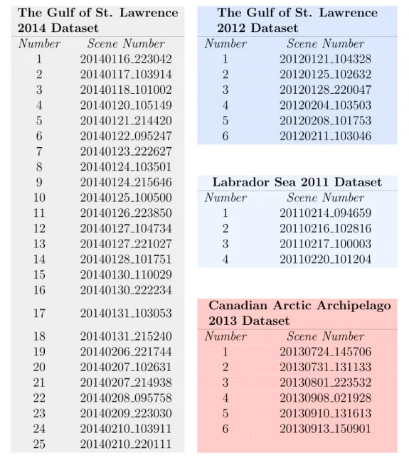
4.1 Image acquisition dates for all images used in the ice concentration estima-tion study . . . 37

4.2 The structure of CNN-based regression model . . . 41

4.3 Hyper-parameters of the CNN . . . 42

4.4 Experimental results from using AICs as compared to HLICs in the training data. Results shown here are for all five folds. The number of patches means the total number of patches extracted from each SAR scene . . . 44

4.5 The comparison of three experiments . . . 46

4.6 Results from experiments using different training datasets . . . 52

4.7 Confusion matrices for the experiments carried out in this study, in addition to those from ASI . . . 56

(10)

List of Figures

2.1 An example of a dual-pol SAR scene . . . 6

2.2 East cost of Canada with the Gulf of Saint Lawrence shown . . . 8

2.3 The architecture of a typical CNN . . . 11

3.1 Example of a 3D image used for extracting patches . . . 23

3.2 Samples of patches with size 45×45×3 . . . 24

3.3 Flowchart of method for sea ice and water classification. . . 26

3.4 Water and sea ice classification results visualization of two SAR scenes . . 32

3.5 An example of a SAR scene with relatively low classification accuracy . . . 33

4.1 Sea ice features in different datasets . . . 38

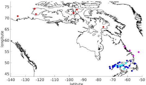
4.2 Geographical location of the datasets used for sea ice concentration estima-tion study . . . 38

4.3 An example of land mirroring . . . 40

4.4 Results visualization for 20140210 103911 from experiments using AICs and HLICs . . . 46

4.5 Results visualization analysis from experiments using AICs versus HLICs . 47 4.6 Ice concentrations prediction distribution calculated based on cross valida-tion results of the entire GSL2014 dataset . . . 48

4.7 Estimation results from the CNN versus image analysis chart . . . 49

4.8 Distribution of ice concentration categories . . . 50

(11)

4.10 An example of results visulization of experiments using different training datasets . . . 54

4.11 Estimation results from CNN models verse ice analysis charts from experi-ments using different datasets . . . 57

A.1 Results visualization for 20140117 103914 from experiments using AICs and HLICs. . . 72

A.2 Results visualization for 20140131 215240 from experiments using AICs and HLICs . . . 73

B.1 Results visualization of 20140116 223042 from experiments using different training datasets . . . 79

(12)

Chapter 1

Introduction

Obtaining knowledge of sea ice is important to understand climate change, as well as for weather forecasting and marine operations in ice covered regions. According to recent studies, sea ice cover is currently undergoing significant changes with an observed decline not only in the extent of multiyear sea ice [7], but also an overall reduction in thickness [39]. The rate of these changes has being increasing in recent years [39]. In order to monitor the condition of sea ice and support safe Arctic operations and navigations in ice-infested waters, effective and high resolution information of the ice coverage is desire [66, 57].

Satellite observations such as synthetic aperture radar (SAR) images are widely used for sea ice information retrieval. These images have high spatial resolution and have the ability to see through cloud cover, and are ideal for sea ice mapping. It is challenging to interpret SAR images since the interactions between the SAR signal and sea ice are affected by various factors, including the imaging frequency and incidence angle, and the surface conditions of sea ice [43,42].

Apart from several physical algorithms that can be applied to retrieve ice information from SAR imagery, machine learning algorithms such as support vector machine (SVM), random forest, and k-nearest neighbour (KNN), combined with hand-crafted features (e.g., geometrical feature [62], Fourier descriptors) also can be adopted to obtain impressive performance on sea ice information retrival. For example, a SVM model trained using SAR image texture features was proposed to identify multiple sea ice types[45].

One approach of machine learning called convolutional neural networks (CNNs) is at-tracting increasing attention in the remote sensing domain because CNNs are now the state-of-the-art for image related tasks [2]. Due to the availability of large datasets and the use of GPUs, which can alleviate the training inefficiency, and some novel approaches

(13)

to reduce over-fitting [75, 38,67], CNNs have been shown to significantly outperform tra-ditional methods for image classification tasks [2]. Due to the success of CNNs on image classification tasks, CNNs are expected to perform well on SAR imagery classification prob-lem as well [23]. In addition, with continuous advancements and developments in satellite technology, the volume of available synthetic aperture radar (SAR) images is increasing, which increases the need for automated algorithms to analyse these images. The objective of this thesis is to apply CNN-based learning approaches for the analysis of sea ice SAR imagery, providing more effective and timely information about sea ice so as to facilitate human activities.

One challenging task in sea ice remote sensing field is to classify sea ice and open water in satellite imagery accurately [84]. Distinguishing sea ice and open water from SAR imagery is critical for many activities, such as ship navigation, search, and rescue operations. Nowadays, automated methods to distinguish sea ice and water in SAR imagery are in demand. CNN-based approach can be used to solve this problem. In this thesis, a CNN-based transfer learning approach is adopted to classify sea ice and open water from SAR images, image features are extracted from a pre-trained CNN and softmax classifier is adopted to achieve final classification of sea ice and water. This approach achieved 92.36% classification accuracy on average after applying cross-validation.

The other topic of this thesis is sea ice concentration estimation. Currently, SAR images are manually interpreted by human experts working in government agencies to pro-duce operational image analysis charts, which display sea ice concentration information over certain regions [75,54]. However, preparation of these charts is very time-consuming and this human visual interpretation tends to be biased. It is of interest to find an intel-ligent and robust method to facilitate the estimation of sea ice concentration from SAR imagery. Although there are numerous methods available, this thesis mainly focuses on sea ice concentration estimation from SAR images by training a CNN model from scratch. However, the ice concentration from this CNN has the same problem as that from Wang [75], which is that the ice concentration in the range of 10% to 80%, is not estimated very accurately.

By looking into the available dataset, the imbalanced dataset problem was discovered and several possible methods to address this problem are proposed. The experimental results show that the efforts of balancing the dataset by introducing minority categories from new datasets do make a difference, even though the sea ice features and SAR image acquisition periods between datasets differ. With the size limitation of available new datasets, the original dataset could not be totally balanced by the new samples introduced by new datasets. However, the results do show an impressive improvement according to many experiments which aim at balancing the original dataset. Moreover, it is found that

(14)

the CNN model outperform other methods on identifying marginal ice zone. This finding is supported by the experiments in this study.

The outline of this thesis is as follows: We first give a brief background introduction in chapter2 of some essential concepts that will be discussed in this thesis. In chapter 3, various data preprocessing methods for most of our experiments are illustrated in detail, and the method of classification of sea ice and water from SAR images is also presented. In chapter4, sea ice concentration estimation by using CNN is discussed and the imbalanced problem is studied.

(15)

Chapter 2

Background

This chapter presents background knowledge related to this thesis. It includes relevant fundamental concepts of remote sensing, such as properties of synthetic aperture radar imagery and sea ice monitoring. In addition, background of convolutional neural networks, and recent research of applying CNN approaches in remote sensing are presented in this chapter. A CNN-based method called transfer learning is introduced as well. Finally, the imbalanced dataset issue is briefly discussed at the end.

2.1

Sea Ice and SAR Introduction

2.1.1

Sea Ice Basics

Monitoring sea ice is crucial for many high latitude countries [63]. Sea ice is a part of the cryosphere, interacting constantly with the underlying ocean and the overlaying atmosphere [9, 63]. Sea ice floats on the ocean’s surface because sea ice is less dense than water [9]. Due to the effects of winds, currents and temperature fluctuations, sea ice is very dynamic in the ocean [9]. Therefore, there are numerous sea ice types, for example, deformed and undeformed sea ice, and various sea ice features, such as pressure ridges or cracks in the sea ice cover, are generated [9].

The percentage of sea ice coverage in a given sea area is defined as sea ice concentration, or ice concentration (IC), ranging from 0% to 100%. The definition of 0% ice concentration means there is no ice but water in the given sea area, while 100% ice concentration means ice is covering all the given area [35].

(16)

The information of sea ice is important for numerous applications. First of all, sea ice can impede ship traffic and increase the risk of traffic accidents in the Arctic [63, 9]. Sea ice is highly related to climate, it can be considered as a climate indicator. For example, reductions in sea ice extent and thickness are believed to be due to warming climate [63,9]. A consolidated ice cover can be regarded as an insulator that hinders the exchange of mass, momentum and chemical constituent between the ocean and the atmosphere [63]. Finally, fluxes at the ice surface provide boundary conditions for weather forecasting models.

2.1.2

SAR Imagery

Synthetic aperture radar (SAR) is widely used for sea ice monitoring. It is well known for its all-day and all-weather sensing capability [30], because it can capture images of the earth surface even through clouds and in total darkness (without sunlight) [17]. Generally speaking, SAR is a form of radar, which is used to create 2D or 3D images of an object or earth’s surface [10]. SAR images are able to represent more details of the ice cover as compared to passive microwave images because of their high spatial resolution [23]. In comparison to the resolution of operational ice concentration products based on passive radiometer data, the resolution of SAR data is significantly higher [35].

Nowadays, the main data source that is used for sea ice monitoring in Canada is RADARSAT-2. RADARSAT-2 has four different polarization configurations for SAR sys-tems:

1. HH: Horizontal polarization on transmit, Horizontal polarization on receive 2. HV: Horizontal polarization on transmit, Vertical polarization on receive 3. VH: Vertical polarization on transmit, Horizontal polarization on receive 4. VV: Vertical polarization on transmit, Vertical polarization on receive

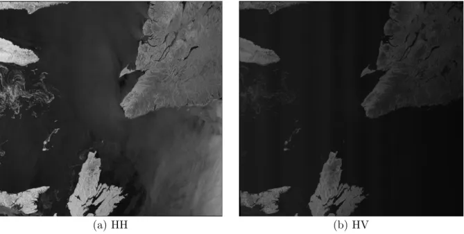
Each polarization configuration corresponds to one SAR image. A dual-pol SAR scene contains two images, one HH and one HV, and covers a large spatial region (approximately 500km x 500km), and it is commonly used for ice charting. In contrast, a quad-pol scene contains four images (HH,HV,VH,VV) and covers a smaller geographic region. Experi-ments in this thesis are based on dual-pol SAR scenes. For example, a dual-pol SAR scene is shown in Figure 2.1. The image 2.1a is HH polarization image, while the image 2.1b is HV polarization image.

(17)

(a) HH (b) HV

Figure 2.1: An example of a dual-pol SAR scene acquired on 2014-01-18 in the Gulf of St. Lawrence.

The ice analysis charts produced by Canadian Ice Service have relied heavily on RADARSAT-2 since it was launched in RADARSAT-2007 [37, 49]. The ongoing satellite misson RADASAT-2 in Canada is presently considered as the most reliable source of information on the condition of sea ice [37].

2.1.3

Sea Ice Monitoring

Many approaches have been developed to monitor sea ice conditions using satellite data. The three most popular data sources are optical sensors, passive microwave sensors, and SAR [27].

Optical sensors have the benefit of relatively fine spatial resolution (1km) but also some shortcomings, image capture conditions are limited by cloud coverage and sun illumination over the Arctic during winter [37]. Thus, the data from optical sensors cannot satisfy the requirements of ice operations because optical sensors only provide data under cloud-free conditions. Other data sources used to monitor sea ice, passive microwave and scatterom-eter observations, are not significantly restricted by clouds and sunlight [37]. The strong contrast of the emissivity of sea ice and water makes water and different sea ice types easily

(18)

distinguished in passive microwave images [3, 75]. However, the low resolution of passive microwave data makes them barely applicable in the vicinity of a shoreline and within narrow channels [37].

Compared to the two data sources discussed above, high-resolution synthetic aperture radar images (nominal pixel spacing less than or equal to 50m) [37] from RADARSAT have been considered as the main data source for ice monitoring in several countries, particularly in Canada [68], who uses large amounts of wide-swath SAR images to monitor Canadian ice regions [63]. This thesis mainly focuses on using SAR imagery to retrieve sea ice information.

2.1.4

Sea Ice Features of The Gulf of St. Lawrence

The main study area of this thesis located in the Gulf of St. Lawrence (GSL), which is a semienclosed sea along the east coast of Canada [74]. A picture of this area is shown in Figure2.2, most of SAR images used for the experiments of this thesis were captured from Gulf of St. Lawrence in the period of January 16, 2014 to February 10, 2014. This time period corresponds to the freeze up stage of sea ice in the Gulf of St. Lawrence.

The sea ice in GSL has strong seasonality and dynamic motion [74]. A typical timeline of sea ice formation in the Gulf of St. Lawrence is as follows: new ice begins to form in the upper of GSL near the end of December, and the ice cover augments in concentration at the beginning of January. Sea ice occurs first in shallow areas at the very begining of the ice season and then spreads eastward [74]. Ice covers almost the entire Gulf of St.Lawrence by the third week of February [16]. Sea ice in the GSL reaches its maximum stage of formation by the third week of March, after that, melting and dispersal procedure begin [74].

Land-fast ice has limited extent in the Gulf of St. Lawrence, and ice moves from shore into the main part of the Gulf of St. Lawrence due to wind and water motion [16]. As a result, floes and some new ice are generated in the central region of the gulf. Wind affects the motion of sea ice significantly in the northeastern of the Gulf of St. Lawrence [16]. Sometimes, very large floes will occur in this area [16]. Sea ice is very mobile in the Gulf of St Lawrence, the size of floes is commomly small [16]. Ridging can be rather extensive in some areas, but not developed to any great height.

(19)

Figure 2.2: East cost of Canada with the Gulf of Saint Lawrence shown. (Source: [8])

2.2

Image Analysis Charts

To provide ice information to customers, the Canadian Ice Service (CIS) relies heavily on SAR imagery [15]. These images will be analysed to create image analysis charts, which are ice maps produced by ice experts from CIS through visual interpretation of SAR imagery [43,42]. The zone analysized by the image analysis concurs with an area relating to the satellite path. Therefore, the satellite’s path varies each day thus the chart area shifts from day to day [15]. According to the official website of Environment and Climate Change Canada (ECCC), around 11,000 SAR images from RADARSAT-2 are received per year [15]. Sea ice experts take approximately 4 hours to analyse a SAR scene [15]. In most cases, analysis results are issued in the form of image analysis charts [15].

To produce image analysis charts, expert analysts visually identify regions in the image that have homogeneous ice conditions and assign an ice concentration label to that region. These labels are assigned in tenths (e.g., 10%, 20% . . . ), and therefore the precision of this ice concentration is normally considered to be approximately 10%.

(20)

experience of visually looking at SAR images, but also their experience of the ice conditions in the region. Analyzing images is particularly challenging if seas are rough, or sometimes if water is on the ice, accumulated either from melt or rainfall [15]. Although image analysis charts are normally considered reliable, there are several source of uncertainty and errors in the image analysis charts because they are based on human interpretation [19]. In addition, the process of generating image analysis charts is time-consuming, that is the reason why automating the process of ice information retrieval is significant [75].

2.3

Convolutional Neural Networks

Convolutional neural networks (CNNs) models have recently been applied to large-scale visual recognition tasks. These networks are trained via backpropagation through layers of convolutional filters [41, 14, 67]. With large quantities of training data, CNN models outperform other models, and had early success in digit classification tasks. Nowadays, many technologies related to CNNs are used in our daily life, for instance, face recognition [51] and machine translation [28]. CNNs are an active area of research and have achieved appealing progresses in many fields, such as medical imaging and automobile industry. However, CNNs are still not widely used in remote sensing, there are still substantial problems that are worth exploring [22]. In this section, we will provide a brief introduction about CNNs, and the algorithm of training a CNN.

2.3.1

Convolutional Neural Networks Basics

CNNs are fundamentally the same as ordinary neural networks, which are comprised of neurons that have weights and biases to be learned [32]. A CNN consists of multiple layers, which are typically convolutional layers, pooling layers, fully-connected layers, and non-linear layers. The arrangement of these layers determines the architecture of a CNN. Normally, each neuron receives some inputs, performs a dot product between the inputs and the filter weights, followed by a non-linearity, which is called the activation function [31]. The most popular activations functions are Sigmoid, Tanh, and ReLU [31]. The convolutional layers are typically followed by fully-connected layers. For a classification problem, these layers provide inputs to a softmax function that computes a probability, and finally a loss function, such as cross-entropy, is used to compare the network outputs to the target outputs [32].

CNN feature learning algorithms have achieved superior performance over hand-designed features in many benchmark data sets [38]. The most salient characteristics of a CNN are

(21)

local connections and parameter sharing. These two characteritics lead to the main ad-vantage of CNNs, which means that the computational cost to train a CNN is reasonable as there are fewer parameters than fully connected networks with the identical number of hidden layers [31].

In recent years, more and more complex CNN models have been developed, for example, AlexNet [38], VGG-16-Net [67], GoogLeNet [71], and the latest one, Res-Net [21], all of them are the champions of ImageNet Large-Scale Visual Recognition Challenge (ILSVRC) respectively in the passing years. Generally speaking, the deeper and wider of a CNN structure, the better the performance it will achieve. However, memory and the computa-tional resources are a challenge when training these CNNs. In addition, to avoid overfitting problem, a considerably large dataset is in demand for deeper and wider CNNs.

2.3.2

The Architecture of Convolutional Neural Networks

A typical CNN consists of a number of convolutional layers, pooling layers optionally followed by several fully-connected layers [58]. As the convolution operation is in charge of the most heavy computation part of a CNN, convolutional layers are regarded as the most important components [31]. The function of convolutional layer is to compute the output of neurons that are connected to local regions in the input, each computing a dot product between their weights and a small region they are connected to in the input volume [58]. The pooling layer basically performs a down sampling operation, while the category scores are computed after the fully-connected layer, where fully-conected means that each neuron in this layer and in the previous layer is connected to each neural in the previous layer. A typical CNN structure is shown in Figure2.3.

2.3.3

Optimization For Convolutional Neural Networks

Neural network training is one of the most difficult optimization problems [18]. Gradient descent is the most commonly used modern optimization algorithm, which follows the gra-dient of the entire training set downhill. Gragra-dient descent may be accelerated significantly by using stochastic gradient descent with fixed learning rate [18]. Instead of using fixed learning rate, numerous algorithms have been proposed that can adapt the leaning rate recently during training [18]. For example, AdaGrad [36], RMSProp [73].

(22)

Figure 2.3: The architecture of a typical CNN. Source:[40]

2.3.4

Model Training

The algorithm that is commonly used to train CNN models is stochastic gradient descent (SGD), which uses backpropagation to compute its gradients [61]. Backpropagation is the most popular algorithm for multi-layer networks, the core of this algorithm is to apply the chain rule to compute the effect of each weight in the network with respect to error function [61]. This algorithm can be applied to effectively compute the gradients for SGD algorithm.

The input samples first propogate through CNN, and then the derivatives of the loss with respect to the parameters throughout the network are computed by backpropaga-tion algorithm. Regarding the optimizabackpropaga-tion method, the weights are updated through mini-batch stochastic gradient descent (SGD) [85]. The objective of SGD algorithm is to minimize the loss function so as to find the optimal parameters in the convolutional network model with a good generalization ability for the target problem. First of all, the general form of cost function J(θ) is defined as follows [18],

J(θ) = L(f(x;θ), y) = 1 m m X i=1 L(f(x(i);θ), y(i)))).

(23)

setθ, where m is the number of samples in the mini-batch, y denotes the desired output or label for each sample.

L2 loss (Euclidean loss) is typically used for CNN-based image regression tasks [77]. In this study, an Euclidean loss layer is adopted at the last layer of the network. Euclidean loss with L2 regularization term has the form [18],

Lf(x;θ),y = 1 2m m X i=0 (f(x(i);θ)−y(i))2 +λ m X i=1 θ_i2.

This function is otherwise called the “squared error function”, or “mean squared error”. The mean is halved for the sake of a convenience for the computation of the gradient descent, as the derivative term of the square function will cancel out the 1/2 term. In order to update weights, the gradient of the loss with respect to the weights is needed [18].

ˆ g = ∂Lf(x;θ),y ∂θ = 1 m m X i=0 (f(x(i);θ)−y(i))∂f(x (i)_;_θ₎ ∂θ + 2λθi.

where ˆg denotes the gradient calculated based on m samples randomly sampled from the training data. The calculated gradient will be used for mini-batch SGD algorithm, updat-ingθin the direction of ˆg, a mini-batch SGD algorithm is based on the following steps [18]. Step 1: Randomly initiate weights θ and set values for hyperparameters.

Step 2: Iterate the followings until stop criteria is met.

Sampling a minibatch m sample{x1, x2, ...xm}from training set and the corresponding labels

y(i)

calculate the gradient: ˆg := 1

m 5θ

X

i

L(f(x(i);θ), y(i))) calculate velocity update: v :=αv−gˆ

update each weight: θ :=θ+v.

wheredenotes learning rate, we usev denotes velocity andα denotes momentum param-eter. The symbol := means to update the parameter on the left side of the symbol by the computed value of the equation on the right side of the symbol. The symbol 5θ denotes

(24)

2.4

Transfer Learning

Training an entire deep CNN from scratch, which means initializing the weights at random, is often impractical in practice, because it is not feasible to obtain a large number of training samples. People normally collect limited datasets with far less than the total parameters in a deep CNN [33], which has millions of parameters that need be determined [23]. However, in particular, there is no large-scale labelled SAR imagery dataset that is widely used to test deep learning algorithms. To balance this trade-off, transfer learning is expected to play a significant role in the case of deep CNNs for tasks using SAR imagery. Transfer learning is an effective way of training a large CNN without overfitting when the dataset is insufficient [23].

The main concept of transfer learning is as follows. First, we need to train a base network on a relatively huge dataset, for example, ImageNet, which contains about 22,000 classes and nearly 15 million labeled images. Second, we reuse the learned weights or features of the pretrained network in a new network that will be used for our dataset (target dataset) [83]. This process will be successful as long as general features are learned well from the original huge base dataset, and the new target database also contains these kind of general features [83]. In practice, numerous studies have implemented this transfer learning method for various tasks, with results that are comparable to those from conventional methods.

There is an interesting common phenomenon that has been observed from many deep CNNs trained on natural images. Typically, simple features, such as Gabor features, edges, and color blobs are learned at the first few layers [33, 83]. Such features are not specific to a particular dataset, they are generic features that will be useful for a variety of image classification and recognition tasks. While this fact is heuristic, it does provide a fundamental theoretical support for applying transfer learning method. However, features detected from the later layers of the neural network are more specific to the base dataset [33]. Therefore, we only need to modify the last few layers to fit target tasks. For most CNNs trained for image classification, we know that the features computed by the network’s last layer must depend greatly on the chosen specific dataset, for example, if a network that has been trained with softmax layer as the last layer, then each output unit will be specific to a particular category [33,83]. This means that if you have 10 classes, then there will be 10 corresponding outputs.

In summary, transfer learning can be summaried as follows: First, to pretrain a CNN on a large dataset, and then use the weights of pretrained CNN either as an initialization of weights or regarding the entire CNN as a fixed feature extractor for new datasets or tasks

(25)

[33]. There are two commonly used transfer learning scenarios which will be presented in the following subsections in detail [33].

2.4.1

Scenario I: Feature Extractor

The basic idea of the first transfer learning scenario is to treat a pre-trained CNN as a fixed feature extractor and retain the classifier [33]. To be more specific, a CNN pretrained on ImageNet is taken, and then removing the last fully-connected layer. After that, we can treat the rest of the CNN as a fixed feature extractor for the target dataset [33]. If we take an AlexNet as an example, this operation will return a 4096-dimension feature vector for every image that is fed through the AlexNet [33]. This feature vector is then used to train a linear classifier, for instance, Linear SVM, KNN, or softmax classifier for the target dataset [33].

2.4.2

Scenario II: Fine-tuning

In addition to the method discussed above, there is another transfer learning method that is popular, which is copying weights from the first several layers of a trained base network to the first several layers of a new network [83]. The remaining layers of the target network are trained using the new dataset with random weights initialization [83]. During training process, there are two options: one options is to backpropagate the errors from the new task into all the layers including the first several layers to fine-tune the copied weights. The other option is keeping copied weights of the first several layers fixed, which means the weights for these layer will remain unchanged during training [83]. As for the remaining several last layers, they will be retrained to be more specific to the new task. The decision whether or not to retrain the first layers not only depends on the size of the new dataset, but also relies on the number of parameters need to be trained in the first several layers [83].

Keeping a portion of the prior layers frozen and fine-tuning the rest of the network is appealing due to overfitting concerns [33]. Overfitting can occur when the new dataset is small and the number of parameters need to be trained is relatively large. In this case, it is better to keep the weights of the majority of the layers unchanged [83]. However, overfitting will not be a problem when the new dataset is sufficient, and in this case tweaking weights of a few layers of the network can boost the performance on the new dataset [83]. In an extreme case, there is no need to do transfer learning if you are confident that the size of the target dataset is sufficient, i.e, datasets that weights are being transferred to is

(26)

big enough. That is because learning from scratch on the large target dataset will give satisfying results without overfitting concerns [83]. However, The computing time of this method is much longer than that of transfer learning.

2.5

Previous Work Relevant To This Thesis

2.5.1

Research on CNNs In Remote Sensing Applications

In recent years, there is a large and growing volume of published studies describing the role of CNNs in different fields. Implementing CNNs algorithms is becoming more popular in the remote sensing community. Studies have shown that CNNs approaches outperform conventional methods in a wide range of tasks, for instance, SAR image depeckling, remote sensing image target recognition, classification, edge detection and so on. In this section, I give a literature review of previous research of applying CNNs approaches in the domain of remote sensing.

The studies of Ot´avio AB et al. [59] demonstrate that CNNs not only can be used to recognize natural objects, but trained CNN models generalizes well on the task of classifying remote sensing scenes. A CNN-based approach for detecting edges in remote sensing images is proposed [81], and found that their approach can detect the continuous edges of remote sensing images and has strong robustness compared with classic algorithms. Jun et al. [13]explicitly explored the ability of a deep CNN with data augmentation on SAR target recognition.

Kampffmeyer et al. [29] proposed a deep CNN for semantic segmantation of urban re-mote sensing images. The results show that they obtain an overall classification accuracy of 87%, this score is higher than the state-of-the-art for the dataset they used. Maggiori et al [48] proposed a four stacked convolutional layers for extracting features and a deconvolu-tional layer as the last layer. This convoludeconvolu-tional network is designed for pixelwise labeling of remote sensing imagery. Their experimental results surpass previous approaches not only in terms of efficiency, but also in terms of accuracy [48].

CNNs are found to be able to deal with SAR image depeckling problems as well. An eight convolutional layer network with a method that similar to residual learning is designed in [6] for SAR image depeckling. The CNN model they proposed was found to outperform three other image despeckling algorithms. In addition, CNNs are also found to be able to tackle the problem of pansharpening remote sensing images. An example can be found in [50].

(27)

One approach that is particularly related to the studies in chapter 3 is the study de-scribed in [44]. They have shown a CNN model can be successfully used on sea ice and water classification task. They directly use polygon-wise ice concentration of image anal-ysis chart, classifying sea ice and open water from SAR imagery based an Alter-CNN algorithm [44]. They obtain impressive results in comparison with other algorithms.

Another study that is similar to our studies presented in chapter 4 is the study pro-posed by Wang [75]. A CNN structure and a fully-convolutional neural network (FCNN) structure taking SAR images and incidence angle as input are developed to estimate sea ice concentration for SAR imagery. Both the FCNN and the CNN models are able to obtain good results even for very thin new ice, which is difficult to distinguish visually in the imagery [75]. The root mean squared errors are 0.22 and 0.21 for CNN and FCNN respectively. The CNN models are found to be able to generate reasonable ice concen-tration in the melt season when evaluating the performance on a Beaufort Sea dataset, and achieved a state-of-the-art ice concentration estimation [75]. Wang also evaluate the transferability of CNN models and found CNN models are transferable between different SAR image datasets [75]. Wang’s works in [75] is the first study in which a CNN is applied to estimate sea ice concentration from SAR images.

2.5.2

Research On Transfer Learning In Remote Sensing

The main approach presently used for transfer learning in remote sensing is using pre-trained CNNs as feature extractors. Morgan et al. [55] explored how a deep CNN approach performs on the classification of SAR imagery, and they conclude that a CNN method can be adapted quickly to new SAR imagery classification tasks [55]. One interesting transfer learning based method was proposed by Huang et al. [23]. They transferred from a tacked convolutional auto-encoders model trained on unlabelled sufficient SAR images to a labelled new dataset with limited number of training SAR images [23]. They report that their method is competitive with the state-of-the-art method on their dataset, and their method performs even better if the size of training sample is small compared to other methods [23].

Kang et al [30] combined an algorithm for SAR ship detection based on transfer learn-ing method. They extracted features of SAR images from VGG [67], they discover that combining pixels and deep feature can boost the performance of multiscale ship detection in SAR images [30].

The method proposed by Castelluccio et al. [4] is similar to the method presented in chapter 3, which is the classification of sea ice and open water from SAR imagery,

(28)

Castelluccio et al. adopted CaffeNet and GoogLeNet, finetuning these pre-trained CNN for semantic classification of remote sensing scenes. In chapter3, transfer learning approach will be illustrated more specifically.

2.6

Research on Imbalanced Datasets

A dataset is regarded as imbalanced when there are significant differences among the number of samples available for each category [5]. An example of an imbalanced dataset is sea ice SAR imagery datasets, which often contain more samples of open water and ice at high concentrations than samples at intermediate ice concentrations.

Obtaining a balanced dataset at the very beginning is not always possible because real-world datasets are more or less imbalanced. If a dataset is imbalanced, the minority categories are not well represented and models will focus more on majority categories during model training. Thus, the prediction ability for these minority categories is weaker compared to majority categories [47].

Coping with imbalanced dataset problem is important in many applications, especially when the primary interest is on the minority categories, such as detection of fraud calls, and filtering fraud transaction in banking operations [60]. Examples for sea ice would be detecting an isolated ice floe, or an opening in a consolidated ice cover.

There are three commonly used methods that can deal with problems caused by imbal-anced datasets. The first two methods are based on sampling method. Intuitively, as our goal is to balance a dataset, sampling methods can help to tackle this kind of problem. One way is oversampling samples in the minority categories, the intent is to increase the number of samples in the minority categories until the number of samples in each category is almost equal before applying machine learning algorithms. However, when applying oversampling algorithm, we cannot just repeatedly get samples from minority categories, because it can lead to overfitting. One classical oversampling method for imbalanced dataset is called SMOTE proposed in [5], the minority categories are oversampled by creating “synthetic” examples rather than by over-sampling with replacement [5]. A“synthetic” example is generated according to the formula,

xi1 =xi+ζ(xnn−xi).

where xi1 is the newly generated“synthetic” sample, xi is the original sample, xnn the

(29)

The second method is undersampling samples in the majority categories [87], i.e, ran-domly removing several samples from majority categories until the number of majority categories is almost as small as the number of samples in the minority categories before applying learning algorithms [87]. Chawla et al. [5] conclude that undersampling method enables better classifier than oversampling method. On the other hand, if we abandon samples from majority categories at random, then important information can be ommited [87, 47].

The third method that can be adopted for addressing imbalanced dataset problem is based on modifing the learning algorithms. For example, support vector machine combined with boosting or ensemble method can perform better than learning from the original im-balanced dataset [47]. Another widely used approach is called cost-sensitive learning [46], which addresses the imbalanced dataset problem through incurring different costs for differ-ent classes. One typical approach of cost-sensitive learning is to move the decision thresh-olds according to their corresponding misclassification costs. To explain this approach in a simple way, assume the imbalanced dataset consists of two classes, a negative category and a positive class. pdenotes the probability estimation results is positive category from a binary classifier, the decision is based on a threshold,

if p

1−p >1; positive class (1)

else; negative class.

However, if the number of positive samples is different from the number of negative samples in the training dataset, then the threshold should be as follows:

if p 1−p >

m+

m−; positive class (2)

else; negative class

wherem+ _{denotes the number of positive samples in the training set and}_m−_{is the number}

of negative samples in the training set.

However, if our classifier is based on (1), then we need to adjust the predicted probability

p when using(1) to make decision, the formula is, if p

1−p× m−

m+ >1; positive class (3)

(30)

This is just a basic idea, we can sort of adjust the predicted probabilities when making decisions. However, it is way more complicated in reality; We need to embed something similar to (3) to decision process [87].

(31)

Chapter 3

Sea Ice And Water Classification Of

SAR Imagery Using Transfer

Learning: Scenario I

Accurate and robust classification methods of sea ice and open water are in demand by ice services worldwide [75, 82]. There are many methods that can be used to indentify ice and water from SAR imagery. CNNs are becoming increasingly popular for image related tasks in many research communities due to availability of large image datasets and high-performance computing systems [38, 67, 82]. As CNNs have achieved great success on many image classification tasks, it is reasonable to investigate if CNNs can be used for the classification of image patches from synthetic aperture radar (SAR) imagery into ice and water [82]. In this chapter, several data preprocessing methods, for instance, image analysis charts interpolation, the generation of patches, are discussed in detail. Furthermore, Scenario I of transfer learning has been implemented by extracting features of the patches from AlexNet and training a softmax classifier. This method achieves an overall classification accuracy of 96.69% based on the held-out test data, and obtained 92.36% classification accuracy after applying leave-one-out evaluation. The objectives of the study in this chapter are as follows:

1. To preprocess orginal data into a form suitable for application of CNN.

2. To develop an automated algorithm for ice and water classification from RADARSAT-2 ScanSAR dual-polarization images by using transfer learning scenario I: feature extractor.

(32)

3. To demonstrate the exact procedure of implementing transfer learning to SAR im-agery classification tasks.

4. To verify and discuss the developed CNN-based transfer learning approach against the ground truth, i.e., image analysis charts from Canadian ice service.

5. To evaluate the CNN model by using holdout method and leave-one-out method.

3.1

Dataset

3.1.1

SAR Scenes

The SAR image dataset used for this study consists of 25 SAR scenes, all of them are dual-polarization SAR images [82]. Each scene consists of HH (horizontal transmit polarization, vertical receive polarization), and an HV (horizontal transmit polarization, horizontal re-ceive polarization) image.

The SAR images were acquired in ScanSAR wide mode of RADARSAT-2, with swath width of 500km and nominal pixel spacing of 50m [82]. The available SAR images were captured from Gulf of St. Lawrence in the period of January 16, 2014 to February 10, 2014, which corresponds to freeze-up. Ice concentration and thickness are increasing from January to February [82]. From the image analysis it is known that the ice cover consists mainly of thin, new, gray and gray-white ice, with thickness less than 30cm [16, 82], and becomes looser approximately 20-50 km from the ice edge [76, 82]. The details of the 25 SAR scenes are shown in Table3.1. Note that some SAR scenes contain mostly land.

(33)

Table 3.1: Detailed information of the GSL2014 dataset ID Scene ID Date Acquired The number of Image Patches(Stride=20) 1 20140116 223042 2014-01-16 66 2 20140117 103914 2014-01-17 579 3 20140118 101002 2014-01-18 2320 4 20140120 105149 2014-01-20 120 5 20140121 214420 2014-01-21 1704 6 20140122 095247 2014-01-22 1332 7 20140123 222627 2014-01-23 146 8 20140124 103501 2014-01-24 946 9 20140124 215646 2014-01-24 2375 10 20140125 100500 2014-01-25 1130 11 20140126 223850 2014-01-26 0 12 20140127 104734 2014-01-27 227 13 20140127 221027 2014-01-27 79 14 20140128 101751 2014-01-28 1572 15 20140130 110029 2014-01-30 7 16 20140130 222234 2014-01-30 257 17 20140131 103053 2014-01-31 1327 18 20140131 215240 2014-01-31 2428 19 20140206 221744 2014-02-06 598 20 20140207 102631 2014-02-07 1705 21 20140207 214938 2014-02-07 86 22 20140208 095758 2014-02-08 2204 23 20140209 223030 2014-02-09 60 24 20140210 103911 2014-02-10 380 25 20140210 220111 2014-02-10 1893

3.2

Data Preprocessing

3.2.1

Incidence Angle Data Processing

It is known that the backscatter in a SAR image is sensitive to the incidence angle of the acquisition [1]. The sensitivity to incidence angle is dependent on wind and associated

(34)

ocean roughness conditions [1]. At steep incidence angles during wind roughened con-ditions, the bright signature seen in the HH channel often makes ice versus open water discrimination difficult [1]. Overall, steep incidence angles are preferred to maximize new and thin ice separability in the HH channel and act as a complement to ice versus open water separation in the HVchannel [1].

The incidence angle data interpolation method in this study is the same as that de-scribed in [75]. The incidence angle data are stored as incidence angle images [75]. These images can be used as the third channel of a image patch (image patches will be explained in the next subsection). Finally, these incidence angle images are rescaled to be in the same data range of SAR imagery.

3.2.2

SAR imagery Processing

SAR images are corrupted with significant multiplicative speckle noise due to the coherent nature of the imaging process [82]. In order to eliminate the influence of noise and reduce the data volume, all the SAR images are sub-sampled by 8 x 8 block averaging [82]. The input of the CNN model used requires 3 dimensional data, such as image data with three color channels (RGB). For this study, the HH polarization image, HV polarization image, and incidence angle information for each pixel are combined together to generate the 3D images. An example is shown in Figure3.1.

Figure 3.1: Example of a 3D image used for extracting patches. This image was acquired on January-17 2014. Source[82]

(35)

3.2.3

Extracting Image Patches

Image patches, with size of 45 pixels×45 pixels×3, are extracted from the downsampled SAR image scenes and incidence angle images [75,82]. A patch size of 45 pixels×45 pixels is chosen because experiments conducted in [75, 82] found the patch size of 45 pixels× 45 pixels is the best option of achieving better performance for the task of ice concentration estimation using a CNN.

The method for extracting patches is to extract one patch every 20 pixels (e.g., with a stride of 20) from HH, HV, and incidence angle image respectively and record the central point ice concentration value of the corresponding image analysis chart [82]. The label of a patch is then defined by thresholding the ice concentration. Points with ice concentration greater than 30% are considered to be ice, while points with ice concentration less than and equal to 30% are considered to be water [82]. 23541 patches in total were obtained after discarding land contaminated patches, which are patches containing land pixels [82]. The number of patches extracted from different SAR scene is shown in Table3.1. Several image patches are shown in Figure3.2. Note that the images shown in Figure 3.2 are not the original patches. These patches are processed in order to observe features. The image patches in the top row are water patches, while the image patches in the bottom row are ice patches. It can be seen that the water patches are visually smoother than the ice patches, and that in some cases it can be difficult to distinguish between the ice and water patches visually [82]. This motivates the use of an intelligent model.

Figure 3.2: Samples of patches with size 45×45×3: Each patch has an associated label from the image analysis chart. The top row are water patches, while the bottom row are ice patches.

(36)

3.2.4

Image Analysis Charts Processing

Image analysis charts from CIS is used as the ground truth. Background materials pertain-ing to image analysis charts have been presented in Section2.2. Since image analysis charts contain information about sea ice concentration, while the experiments in this chapter aim to classify sea ice and open water, the image analysis charts are modified by thresholding ice concentration at 30% [82].

Note that there will not be a corresponding ice concentration value (ground truth) from the image analysis chart for every ocean pixel of a specific HH image, because the spatial resolution of the SAR image is much finer than the image analysis chart. Therefore, interpolation of the image analysis ice concentration to the pixel locations in the SAR imagery is necessary. To deal with this problem, nearest neighbour interpolation method is adopted, which interpolates ice concentration from image analysis charts for every ocean pixels based on closest latitude and longitude of original ice analysis charts. However, this also introduces the assumption that the image analysis can be interpreted as valid at this finer spatial resolution.

3.3

Feature Extraction and Classification Method

In this study, instead of building a CNN from scratch, a CNN that has been constructed in an earlier study (AlexNet [38, 82]) is used in a transfer learning approach [83]to classify ice and water in SAR imagery. AlexNet was designed and trained for the task of labelling images from the ImageNet Large-Scale Visual Recognition Challenge (ILSVRC) database. These are images of everyday entities, such as a dog, cat or car, and are significantly different from SAR sea ice imagery [82]. Nevertheless, the experimental results support the use of such an approach for this task [82].

The experiments in this chapter start with the bundled CaffeNet model, which is based on the network architecture of Krizhevsky et al. [38] for ImageNet called AlexNet. From this, the generalization ability of the network is explained when retraining the softmax classifier on the top [82]. To do this, a transfer learning method is adopted. The labelled image patches are fed through AlexNet, which is used as a fixed feature extractor [82]. Features from the sixth fully-connected layer (FC6) of AlexNet are used in a softmax classifier that was retrained to estimate the probability of ice for the center pixel of the patches [82]. In this way, sea ice and open water can be classified [82]. The classification accuracy can be determined by comparing the estimation results to the labels of the testing

(37)

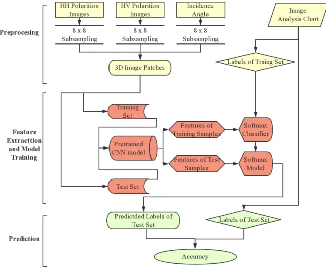
set [82]. The main method is shown in a flowchart in Figure 3.3. In short, this method basically consists of three steps: preprocessing, feature extraction, and prediction [82].

Figure 3.3: Flowchart of method for sea ice and water classification.

3.4

Model Evaluation Methods

In order to evaluate the performance of the model in this study, two methods are adopted for estimating the generalization error depending on different training and testing splits.

(38)

One is called holdout method, the other is called leave-one-out, which is a special variant of cross-validation method.

3.4.1

Holdout Method

Holdout method is relatively easy to understand, the target dataset with labeled samples is divided into two independent sets, namely, the training set and the test set [72]. After obtaining a classification model only using the training set, we evaluate the performance of the model on the test set to obtain an independent estimation of classification accuracy [72]. The percentage of samples in the dataset for training and for testing is typically 80 percent and 20 percent respectively [72].

The holdout method has several shortcomings. First of all, when 20% of the samples are reserved for test set, the number of training samples might be insufficient if the model we want to train is very complex [72]. Thus, the model trained by 80% of the dataset may not be as good as a model trained by all the samples. In addition, the model may be highly dependent on the way the training set and test set are structured [72]. On the other hand, it is a kind of trade-off, when we decide to use a large training set, then the test set must be small for a limited dataset. As a result, the computed classification accuracy from the test set is no longer reliable [72].

3.4.2

Leave-one-out Method

Leave-one-out method is an variant of cross-validation method. It involves using one observation as the test set and the rest of observations as the training set. In terms of this study, one SAR scene was chosen as test set each time, and the remaining SAR scenes are used for training. This is repeated for each image in the set, or 25 times. Leave-one-out approach has the advantage of utilizing as much data as possible for training. In addition, the test sets are mutually exclusive and they effectively cover the entire data set. The drawback of this approach is that it is computationally expensive.

3.5

Experimental Setup

In these experiments, stride of 20 was used between image patches when extracting patches from SAR images, which means spacing between patches is 20x400m or 8km [82]. The

(39)

spacing of image analysis pixels is 8km x 5km [82]. Therefore, this model will not provide prediction for every pixel in a SAR image [82]. In addition, pixels near image borders are unclassified as it is not possible to extract 45 x 45 patches around image border. Moreover, pixels near land boundaries are not classified to avoid contamination of the dataset with unphysical values.

In terms of the holdout method, the first 20 SAR scenes in Table 3.1 were chosen as training data (18918 patches), and the last five scenes were used as the test data (4623 patches). In terms of the leave-one-out method, each scene will be regarded as test set once. As there are no patches extracted from scene 20140126 223850 due to landcover, 24-fold cross validation is executed. The softmax classifier was trained by using a large set of labelled images patches{xi, yi}, wherexi represents inputs image patches,yi represents labels of image patches. A cross-entropy loss function, a typical loss function for image classification, is used for the comparison between the true distributionpand the estimated distribution q, the mathematical expression of cross-entropy has this form, [34]

H(p, q) = −P

xp(x) log q(x).

Softmax classifier produces the probabilty distribution of each class. As the estimated category probability q of the i-th category from the softmax classifier is defined as [34],

qi = e

fyi

P

jefj

.

and fj mean the j-th element of the vector of category scores [34]. Softmax function is a

standard way to turn numbers to probability distributions.

3.6

Results

Measuring the performance of the model on an independent test set is very useful because such a measure provides an unbiased estimate of its generalization error [72]. On the same domain, the accuracy or error rate computed from the test set can also be used to compare the relative performance of classifiers [72]. In this study, we use classification accuracy to measure model performance. Classification accuracy has the following definition:

Classification Accuracy = Number of correct predictions Total number of predictions

(40)

In order to evaluate the performance of the model in this study, the two model evalu-ation methods discussed in Section3.4 are adopted for estimating the generalization error depending on different training and testing splits. Results of both methods will be shown in the following two subsections. At the last part of this section, several conclusions are presented by comparing classification results with image analysis charts.

3.6.1

Holdout Results

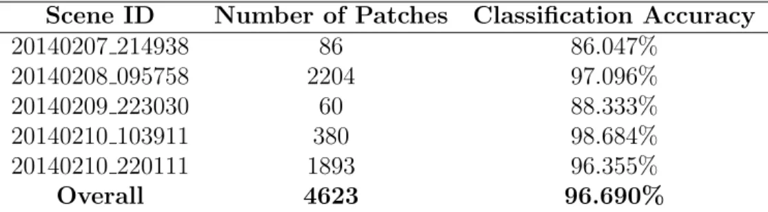
In the experiments carried out here by calculating the number of patches extracted from each SAR scenes, the dataset is split such that around 80% is used for training, and 20% is used for testing, corresponding to five SAR scenes used for testing, and the remaining SAR scenes used for training. Table3.2 below displays the classification results on the five test scenes. It can be clearly observed from table that the overall classification accuracy is around 96.690%. Some SAR scenes have even more accurate classification results. It can be seen in Table3.2 that when a SAR scene has fewer patches, the classification accuracy is relatively lower. One reason for this may be that the classification results on small test set may not represent the real performance of the trained model, if the data in the test set are not well represented in the training data.

Table 3.2: Holdout results for ice-water classification for SAR scenes in the test set using transfer learning. Number of patches means the total number of patches extracted from each SAR scene in the test set.

Scene ID Number of Patches Classification Accuracy

20140207 214938 86 86.047% 20140208 095758 2204 97.096% 20140209 223030 60 88.333% 20140210 103911 380 98.684% 20140210 220111 1893 96.355% Overall 4623 96.690%

(41)

3.6.2

Leave-one-out Results

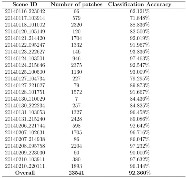
Table 3.3: Leave-one-out results for ice-water classification for the GSL2014 dataset using transfer learning. Number of patches means the total number of patches extracted from each SAR scene

Scene ID Number of patches Classification Accuracy

20140116 223042 66 62.121% 20140117 103914 579 71.848% 20140118 101002 2320 88.836% 20140120 105149 120 82.500% 20140121 214420 1704 92.019% 20140122 095247 1332 91.967% 20140123 222627 146 93.836% 20140124 103501 946 97.463% 20140124 215646 2375 92.547% 20140125 100500 1130 93.009% 20140127 104734 227 79.295% 20140127 221027 79 89.873% 20140128 101751 1572 91.667% 20140130 110029 7 84.436% 20140130 222234 257 84.825% 20140131 103053 1327 96.458% 20140131 215240 2428 89.086% 20140206 221744 598 92.642% 20140207 102631 1705 96.716% 20140207 214938 86 86.047% 20140208 095758 2204 97.232% 20140209 223030 60 90.000% 20140210 103911 380 97.632% 20140210 220111 1893 96.144% Overall 23541 92.360%

Results for the leave-one-out experiments are shown in Table3.3. By averaging the classi-fication results of every experiment weighted by the number of patches in the test image, around 92.3% classification accuracy is achieved. Although this overall classification

(42)

accu-racy is lower than the classification computed by hold-out method, it is still very impressive. According to these results, we can conclude that the method proposed in this chapter per-forms well on our dataset and it also has a good generalization ability. In contrast, Leigh [42] et al. developed a ice-water classification system named MAp-Guided Ice Classification (MAGIC) with an impressive leave-one-out classification accuracy with 96.42%. A paper [84] investigated sea ice and water classification and proposed a SVM based method by using hand-crafted texture features, their method achieved average 91%±4% classification accuracy on validation SAR scenes.

3.6.3

Results Visualization

In order to present the classification results for visualization, the image patches are mapped back to the HH pol SAR image, and are compared with the image analysis charts. Examples are shown in Figure3.4 and Figure 3.5.

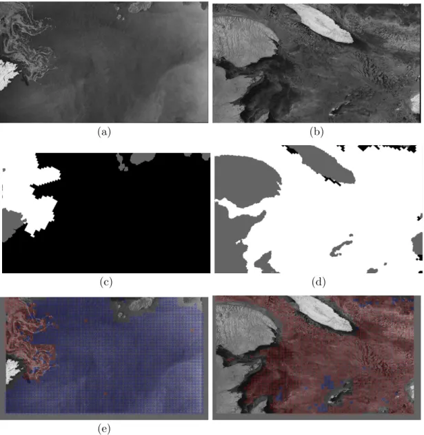
In Figure3.4, two sub-images of two SAR scenes with high classification results (97.232% and 96.144% respectively) are exhibited. The two pictures at the first row are SAR images in HH pol. The two images in the middle are corresponding image analysis charts after thresholding ice concentration. Pixels near land and image boundary are unclassified be-cause the method has not been developed to extract sea ice or water patches from these region. According to Figure 3.4, the classification results are fairly good compared with image analysis charts. Many of the misclassified points are close to the ice edge, i.e., the ice-water boundary. There are only a few misclassified pixels in the open water and ice cover regions respectively, indicating that the method can distinguish both sea ice and open water equally well.

Apart from looking at SAR scenes with high classification accuracies, it is also of interest to look into a SAR scene with relatively low classification accuracy to help us understand cases where the model does not perform well. Figure 3.5 presents a sub-image of a SAR scene with 89% classification accuracy, highlighting the region with classification errors. We can clearly find that the main errors made by model are near ice water boundary, some regions identified as water by the image analysis chart are classified as ice. One interesting finding is that the region highlighted by a yellow circle. This region contains low ice concentration (mainly consists of water) according to ice analysis chart and HH pol image, while the predicted results show that that area mainly consists of sea ice. It seems that the model classification ability for low ice concentration region is not that good. Adding more training samples with low ice concentration might help in this case.

(43)

(a) (b)

(c) (d)

(e)

Figure 3.4: Water and sea ice classification results visualization of two SAR scenes. Source[82], (a), (c), (e) are HH pol image, ground truth, and prediction results of SAR scene (ID: 20140208 095758) respectively; (b), (d), (f) are HH pol image, ground truth, and prediction results of SAR scene (ID: 20140210 220111) respectively. For plots (c) and (d), white represents sea ice, black stands for open water, grey areas are unclassified areas because these are land. The two images at bottom are classification result plots, red circle and blue circle represent sea ice and open water respectively.

(44)

(a) (b)

Figure 3.5: An example of a SAR scene with relatively low classification accuracy. This is a sub-image of Scene ID: 20140131 215240. (a) The corresponding image analysis chart, white represents sea ice, black represents open water, grey represents land and unclassified area. (b) Classification results mapped on SAR image in HH pol, red circle: sea ice. blue circle: water, the yellow circle highlights a region of interest.

(45)

3.7

Discussion

By comparing the classification results with image analysis charts, it can be found that regions near sea ice and water boundary tend to be misclassified. The weak ability to classify pixels near sea ice and water boundary might caused by the way we assign labels for each patch. As the models are trained to estimate the label of the central pixel of a patch, when giving a label for one patch of size 45×45×3, we just assign the label of the center pixel as the label for the whole patch. This label assignment method potentially introduced errors because it might assign wrong labels for some patches. For example, if most of the pixels in one patch are water, but the center point is regarded as sea ice according to a image analysis chart, then the whole patch will be labelled as sea ice, while the true label for this patch should be water.

Note that some of these misclassifications could be due to errors in the image analy-ses, or due differences in how information is represented in image analyses (polygons) as compared to our method (image patches).

Some points near land and near image borders are unclassified as well, which might be a concern if information in these regions is desired. One method to address this problem will be discussed in the next Chapter.

(46)

Chapter 4

Sea Ice Concentration Estimation

Using CNN-based Regression

The previous chapter presented a method to classify pixels in SAR sea ice imagery as ice and water. In this chapter, the problem of sea ice concentration estimation from SAR imagery is addressed.

Accurate sea ice concentration information is important for the human population. Sea ice has an impact on weather and climate. For example, the amount of heat transfered through the ice is directly dependent on the ice concentration [78]. The information of marginal ice zone is also of interest because it is an indicator of Arctic warming and it provides a nice living environment for phytoplankton and creatures such as seabirds and zooplankton [24]. Sea ice concentration also plays an important role in ship navigation. Navigators depend on sea ice concentration charts to find safe routes for icebreakers and ships [78]. For example, regions with low sea ice concentration are passable for many ships while regions with high ice concentration could be very dangerous. Sea ice concentration estimation from SAR imagery is currently done manually by experts working at the Cana-dian Ice Service. However, these ice charts often lack the small scale details of the ice cover, such as individual floes or openings. It is of interest to develop a method to automatically estimate ice concentration from SAR imagery that contains the relevant details.

Different from hand-crafted feature extraction based methods, CNN-based methods learn features from a dataset automatically [23], which can be a good fit for this sea ice concentration estimation problem. In this Chapter, a CNN-based regression model is developed for estimating sea ice concentration based on dual-polarization images (HH and HV), combined with incidence angle image. The model is similar to that used in an earlier

(47)

study [75], although the testing method used here is more thorough. In addition, various experiments are carried out to investigate the role of the training data on the estimation of intermediate ice concentrations (those between 10% and 80%). This will be referred to addressing the imbalanced data problem. Before applying CNN regression models, several data preprocessing techniques, for examples, land mirroring, are discussed in this Chapter.

4.1