.
Diagnostics and Simulation-Based
Methods for Validating Gaussian
Process Emulators
Younus Al-Taweel
Thesis submitted to the University of Sheffield
for the degree of Doctor of Philosophy
University of Sheffield
School of Mathematics and Statistics
Supervisor: Jeremy Oakley
Acknowledgements
I would like to sincerely thank my supervisor Professor Jeremy Oakley for the support and the encouragement that he has given me during my PhD studies. I am thankful for the help and knowledge he has provided me with to enable me to complete my PhD thesis. This thesis could not have been completed without his generous and professional assistance. I also wish to express my sincere thanks to my advisor Dr. Kevin Walters for his guidance and support. I would like also to thank the staff and postgraduate students of the Mathematics and Statistics department for being helpful and friendly at all times. I especially thank my mother, brothers and sisters for their support, prayers and for their entire love. Many thanks to my wife and my family who support me at all times. I would like to thank my uncles, Aqeel and Abdulrahman, and my cousin Naktal. Finally, I would like to also thank all my friends in particular Arqam for being supportive, and providing me with the friendship that I needed during my studies.
I also acknowledge The Higher Committee For Education Development in Iraq for funding of my studentship research and thank all its members for their support. I would also like to thank the department of Mathematics, the College of Education for Pure Science, the Mosul University, the Ministry of Higher Ed-ucation and Scientific Research in Iraq for giving me the opportunity to obtain the PhD degree.
Emulation is a statistical technique that can be utilised for estimating model simulations when the computer models are too computationally expensive to run. Emulators need to be subjected to a validation process since various assumptions have to be made. One assumption is that the computer model output is thought of as a realization of a Gaussian process with a mean and a covariance function. The computer model, however, is not a random sample from the Gaussian process distribution. In this thesis, we develop a graphical diagnostic that can be used to investigate whether the Gaussian process assumption is suitable for building emulators.
Diagnostic methods can be used to assess the validity of the statistical model in order to investigate the best probability model for describing the computer model. However, it is not always possible to derive the required reference dis-tribution for some diagnostics analytically. In this thesis, a simulation-based method is developed based on simulating samples from the posterior distribution of the output function. This simulation-based method can be used to obtain the reference distribution of diagnostics that cannot be obtained analytically. The ob-served diagnostic values will be ‘consistent’ with the simulated diagnostic values if the Gaussian process emulator is valid.
Contents
Acknowledgements iii
Abstract iv
1 Introduction 1
1.1 Computer models . . . 1
1.2 Applications of computer models . . . 2
1.3 The need for surrogate models . . . 3
1.4 Outline of the thesis . . . 5
2 Statistical inference for complex simulators using emulators 8 2.1 Introduction . . . 8
2.2 Emulators . . . 9
2.3 Gaussian process emulators . . . 19
2.3.1 Gaussian process . . . 19 v
2.3.2 The covariance functions . . . 21
2.3.3 Constructing Gaussian process emulators . . . 24
2.4 Inference for Gaussian process parameters . . . 27
2.4.1 Estimating correlation length parameters using the poste-rior mode . . . 28
2.4.2 Markov Chain Monte Carlo algorithm . . . 29
2.4.3 Cross-validation method . . . 31
2.5 Designs for building emulators . . . 31
2.5.1 Latin hypercube design . . . 32
2.5.2 Sliced Latin hypercube design . . . 33
2.5.3 Distance-Based designs . . . 38
2.5.4 Other space-filling designs . . . 38
2.6 Example . . . 40
2.7 Summary . . . 42
3 Validating Gaussian process emulators 43 3.1 Introduction . . . 43
3.2 Uncertainty calibration in emulators . . . 44
3.3 Situations of inappropriate assumptions in building Gaussian pro-cess emulators . . . 46
CONTENTS vii
3.4 Diagnostic methods for Gaussian process emulators . . . 47
3.4.1 Cross-validation method . . . 49
3.4.2 Simple diagnostic methods . . . 50
3.4.3 Diagnostic methods that measure uncertainty . . . 53
3.5 Illustrative examples . . . 61
3.5.1 Borehole model . . . 61
3.5.2 OTL Circuit function . . . 62
3.5.3 Piston Simulation function . . . 62
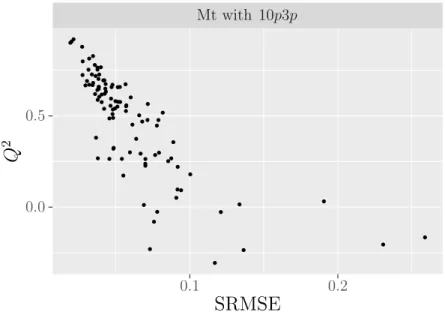
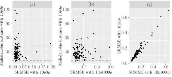
3.5.4 Multivariate Student-t simulator (Mt) . . . 63
3.5.5 Nonstationary variance simulator (NSV) . . . 64
3.5.6 A Gaussian process simulator (GP) . . . 65
3.5.7 Evaluating some diagnostics for the emulators . . . 71
3.6 Conclusion and recommendations . . . 85
4 A simulation-based method and the coverage interval diagnostic 87 4.1 Introduction . . . 87
4.2 The coverage interval diagnostic using separate validation sets . . 88
4.3 The coverage interval diagnostic using the cross-validation method 91 4.3.1 Validating the prior assumptions rather than the posterior emulator . . . 93
4.3.2 Investigating the distribution of p(KαCICV(y)|δˆ) . . . 94
4.4 Quantile-quantile (QQ) plots . . . 96
4.4.1 Example . . . 96
4.5 Simulation-based method . . . 100
4.5.1 The simulation-based method for diagnostics . . . 101
4.5.2 The simulation-based method for the coverage interval di-agnostic using separate validation sets . . . 102
4.5.3 The simulation-based method for the coverage interval di-agnostic using the cross-validation method . . . 104
4.6 Illustrative example . . . 106
4.7 The coverage interval diagnostic with data from a multivariate Student-t distribution . . . 113
4.7.1 Building a Gaussian process emulator . . . 114
4.8 Nonstationary variance simulator (NSV) . . . 124
4.8.1 Building a Gaussian process emulator . . . 125
4.9 Conclusion . . . 133
4.A Appendix A . . . 134 4.A.1 Using simulation to estimate the distribution of KαCICV(·) 134
CONTENTS ix
5.1 Introduction . . . 138
5.2 Treed Gaussian process emulators . . . 140
5.2.1 Constructing TGP emulators . . . 140
5.2.2 Estimating the parameters . . . 143
5.2.3 Predictions of TGP emulators . . . 143
5.2.4 One-dimensional synthetic example . . . 145
5.3 Composite Gaussian process emulators . . . 149
5.3.1 Improving the mean model . . . 150
5.3.2 Improving both the mean and variance models . . . 152
5.3.3 Estimating the parameters . . . 155
5.3.4 Example . . . 156
5.4 The coverage interval diagnostic for TGP and CGP models . . . . 160
5.5 Modified borehole model illustrative example . . . 163
5.5.1 The coverage interval diagnostic for the Modified borehole model . . . 165
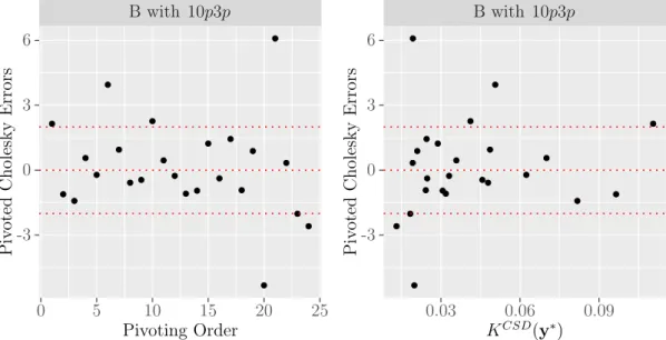
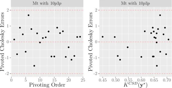
5.5.2 The plot of pivoted Cholesky errors and the scaled condi-tional standard deviations . . . 172
5.6 Conclusion . . . 177
6.2 The relationship between diagnostics . . . 181 6.3 Recommendations . . . 182 6.4 Future work . . . 183
Chapter 1
Introduction
1.1
Computer models
In recent years, computer experiments have increasingly been used as replace-ments for physical experireplace-ments which are considered impractical, impossible or too costly. In order to perform a computer experiment, it is necessary to construct a computer model, called a simulator, which is a mathematical representation of the real system and is usually implemented on a computer. We consider a de-terministic simulator, i.e. one that will produce the same outputs if it is run at the same inputs. The process of running the simulator at different input values is known as a computer experiment. Mathematically, the simulator is referred to as a function, y = f(x) for x ∈ χ ⊂ Rp, where x = (x
1, . . . , xp) is a vector of
inputs and the output is a scalar, y∈R. Typically, simulators will have multiple outputs but in this thesis we focus on single output simulators. Some simulators may also be stochastic, but we do not consider this here.
1.2
Applications of computer models
Computer models have widely been used to investigate the systems of the real world in most science and technology fields. For example, in engineering, Amiri (2012) used the CMG STARS reservoir simulator (Computer Modelling Grup) to simulate low-frequency electrical heating for different models. This simula-tor models multicomponent thermal flow under electrical heating. Vitsas (2016) used a commercial flight simulator, called X-P lane Flight Simulator 10. This simulator gives the user the opportunity for flying different military, commercial and unconventional experimental aircraft over global scenery which covers most geographical areas on the Earth.
In climate and environment, the pCNEM (probabilistic Canadian NAAQS (National Ambient Air Quality Standards) Exposure Model) simulator was de-veloped by Zidek et al. (2005). The pCNEM simulator generates a pollutant concentrations sequence to which a randomly chosen person is exposed over time. Crookston et al. (2010) modified a Climate Forest Vegetation Simulator (Climate-FVS) that provides a useful tool for forest managers. The Climate-FVS model incorporates the potential impacts of climate change in forest plans. The Climate-FVS model also simulates the potential impacts of climate change on various climatically diverse landscapes.
Spracklen et al. (2005) developed the Global Model of Aerosol Processes (GLOMAP) to be an extension of a chemical transport model. The GLOMAP generates the evolution of the global aerosol size distribution. This model also involves the processes of aerosol nucleation, condensation, wet and dry deposi-tion and cloud processing. Emanuel (2002) constructed a relatively simple climate simulator consisting of a single ocean layer and a two-layer atmosphere. This
sim-CHAPTER 1. INTRODUCTION 3 ple climate simulator is able to produce multiple overlapping stable equilibrium states based on a few feedback processes.
Weaver et al. (2001) developed the University of Victoria (UVic) Earth System Climate Model consisting of an energy-moisture balance atmospheric model, a dynamic-thermodynamic sea-ice model and an ocean general circulation model. This model can capture the pathways of bottom, deep and intermediate waters as revealed via simulations which involve the passive tracers release. The model also generates routes of the warm and cold water by returning the upper layer water to the Atlantic Ocean to compensate for North Atlantic Deep Water production and export.
In health, Jandarov et al. (2014) developed an epidemic model that involves a formulation for the spatial transmission among various host cities. This model describes spatiotemporal patterns of epidemics and can accommodate small pop-ulation sizes and disease recolonization. In poppop-ulation, Baggaley et al. (2012b) considered a wavefront model for the spread of Neolithic culture across Europe. The wavefront model allows both an isotropic background spread that incorpo-rates the impacts of local geography, and a localized anisotropic spread connected with major waterways.
1.3
The need for surrogate models
Computer models can be computationally very expensive to run. This means that it can take many hours or even several days to return a value of y at a single of x. Therefore, the simulator can only be run at a limited number of inputs. The computationally expensive problem can be caused, for example, by
the simulator being very complex or a high degree of precision being required. Gaussian process emulators have been widely used as surrogates of computer models in many fields of science and technology. The first use of Gaussian pro-cess emulators as surrogates of computer models was by Sacks et al. (1989b). They present a description of how statistical inference can be used in computer modelling for estimating simulators. Currin et al. (1991) developed the concept of emulators under a Bayesian framework. Gaussian process emulators can be used not only to provide approximations for computationally expensive computer models, but also to provide a probability distribution for the computer models. This probability distribution can be then used to run any subsequent analysis of the computer models.
In certain situations, the statistical assumptions that are made in building Gaussian process emulators may not be precisely satisfied. If the assumptions do not hold, the results that depend on emulators will not be accurate. Hence, Gaussian process emulators are required to be subjected to a validation process using appropriate diagnostics. Some diagnostic methods are just based on the differences between emulator predictions and the simulator outputs. Other diag-nostic methods consider the uncertainty in the emulator predictions. Bastos and O’Hagan (2009) propose a number of numerical and graphical diagnostic methods that take into account uncertainty in the emulator predictions. Their diagnostics are based on comparisons between the validation outputs of the simulator and the emulator predictions. Bastos and O’Hagan (2009) propose comparing the observed value of the diagnostic with its distribution.
In this thesis, we aim to extend the work that is given by Bastos and O’Hagan (2009) for diagnostic methods that consider the uncertainty in the emulator pre-dictions. We evaluate the performance of current diagnostic methods for
examin-CHAPTER 1. INTRODUCTION 5 ing assumptions that are made in constructing Gaussian process emulators. We apply these diagnostic methods on emulators that are built on different simula-tors that have different behaviours. We also present a modification of an existing graphical diagnostic method which makes the diagnostic more informative. We develop a graphical diagnostic method that tests coverage properties of Gaus-sian process emulators. Another contribution is developing a simulation-based method that can be used to obtain the distribution of any diagnostic and it may be applied when the diagnostic distribution cannot be found analytically.
1.4
Outline of the thesis
The focus of this thesis lies in diagnostic methods for examining assumptions that are made in building Gaussian process emulators. The thesis consists of six chapters:
• In Chapter 2, we review literature on applications of Gaussian process em-ulators in several areas of science. The aim is to see what choices authors have made for the mean and the covariance functions when building Gaus-sian process emulators. Furthermore, we want to find the popular designs for generating the design points, the most popular methods that authors used for estimating the correlation length parameters, and the most pop-ular method that authors prefer to use for validating their emulators: the cross-validation methods or separate validation sets. In addition, we aim to investigate what diagnostic methods have been used for validating Gaussian process emulators. The processes of constructing emulators, as surrogates of simulators, under a Bayesian framework are reviewed. We also review several methods used for estimating the correlation parameters in the
cor-relation function. Then, several designs for training and validation inputs that have been used in building Gaussian process emulators are reviewed. • In Chapter 3, the concept of uncertainty calibration in Gaussian process
emulators is described in terms of overconfidence and underconfidence of emulators. We also present the concept of diagnostics and develop a modifi-cation of an existing diagnostic that makes the diagnostic more informative. We investigate the performance of a number of current diagnostic methods for examining assumptions that are made in constructing Gaussian process emulators.
• In Chapter 4, we focus on the development of a graphical diagnostic method that examines coverage properties of Gaussian process emulators. In addi-tion, since the distribution of some diagnostic methods cannot be derived analytically, we develop a method, called simulation-based method, that can be used to obtain the distribution of any diagnostic. We also investigate the performance of our diagnostics with data that have different properties to that of a Gaussian process.
• Stationary Gaussian process emulators have been used widely in the litera-ture. However, the stationary assumption for building Gaussian process emulators may not be suitable for functions that show discontinuity or nonstationary in their behaviour. In Chapter 5, two types of ‘advanced’ Gaussian process emulators that were used for dealing with nonstationary functions are reviewed. These advanced Gaussian process emulators are built under a Bayesian framework. It is necessary to test whether the Gaus-sian process assumption is suitable for building these advanced GausGaus-sian process emulators or not. We also investigate the performance of diagnostic methods for these advanced Gaussian process emulators.
CHAPTER 1. INTRODUCTION 7 • Finally, the conclusion and recommendations of this study as well as ideas
Statistical inference for complex
simulators using emulators
2.1
Introduction
In this chapter, we review a well-known statistical method, called emulation, for tackling the problem of computationally expensive simulators and predicting outputs of simulators. We explain the concept of emulators and present the processes of building emulators under a Bayesian framework. We present various methods for estimating the correlation parameters in the correlation function. We also review some designs for choosing the training and validation inputs. We also present literature search for Gaussian process emulators. Finally, we consider an example as an illustration of Gaussian process emulators.
CHAPTER 2. STATISTICAL INFERENCE FOR COMPLEX
SIMULATORS USING EMULATORS 9
2.2
Emulators
Statistical inference can be used in computer modelling to provide approxi-mations of simulators. The simulator is a function, f(·), where for an input
x = (x1, . . . , xp) ∈ χ ⊂ Rp, the output is y = f(x). Suppose we have a set
of inputs, x1, . . . ,xn, and evaluations y = {y1 = f(x1), . . . , yn = f(xn)} of the
simulator outputs at these inputs. Now, suppose we wish to run the simulator at more values of inputs, but cannot do so because the simulator can be com-putational very expense to run. Thus, we wish to make joint inferences about a set of simulator outputs yn+1 =f(xn+1), yn+2 =f(xn+2), . . . given the available
evaluations of simulator outputs, y.
We consider f(·) to be an uncertain function, in that the simulator output f(x) is unknown before running the simulator at the untried input valuex. Then, we can use a Bayesian perspective to construct a probability distribution for f(·) based on y, and quantify the uncertainty about f(·) due to running the simulator at a limited number of inputs. We call this probability distribution an emulator which can be then used to run any subsequent analysis of the simulator. In fact, this problem can be entirely perceived as a statistical regression problem and any regression model can be used for constructing emulators.
The idea of emulators was proposed by Sacks et al. (1989b) and Currin et al. (1991) developed the concept of emulators using a Bayesian framework. Emula-tors have been used widely in various applications in most science and technology fields. In order to find applications of Gaussian process emulators, we searched the Web of Science (formerly Web of Knowledge) under the terms ‘Gaussian process emulator’, ‘Gaussian process metamodel’, ‘Gaussian process model’ and ‘Gaussian process regression’ according to the following strategy:
1. We used the quotation marks to make our search more accurate.
2. As of 17/10/2017, we found about 1230 studies under the term ‘Gaus-sian process regression’ and 299 studies under the term ‘Gaus‘Gaus-sian process model’. We read the titles and abstracts of some papers that were thought to be relevant to our topic.
3. We found about 71 studies under the terms ‘Gaussian process metamodel’ and ‘Gaussian process emulator’. We focused on papers with mostly dif-ferent authors in order to see difference between methods and applications, because some authors may use the same methodology in their papers. For example, some authors used the same forms of the mean and the covari-ance functions, the same design and the same method for estimating the correlation parameters in their publications.
4. We also added some other papers that were referred to in some of these studies because they contain some detail and some of them used different methodology.
The aim of this search is to find what choices authors have made when building Gaussian process emulators. For example, what they have used for the mean and the covariance functions1and what are the most popular forms of these functions.
Furthermore, we want to find the designs that have been used for generating the design points, for example, the Latin hypercube design (LHD) and the sliced Latin hypercube design (SLHD). Also, we want to find the most popular methods that authors used for estimating the correlation length parameters such as the maximum likelihood estimate (MLE) and a Markov Chain Monte Carlo (MCMC) algorithm. In addition, we want to see which method that authors prefer to use
CHAPTER 2. STATISTICAL INFERENCE FOR COMPLEX
SIMULATORS USING EMULATORS 11
for validating their emulators: the cross-validation methods or separate validation sets. Finally, we aim to find diagnostic methods that have been used for validating their emulators. Some authors use diagnostics that depend only on the difference between the simulator outputs and the emulator predictions such as the mean squared error (MSE), the root mean squared error (RMSE), the standardised root mean squared error (SRMSE) and the predictivity coefficient (Q2). Some other authors use diagnostic methods that consider the uncertainty in the emulator predictions such as the Mahalanobis distance and the individual standardised errors. Table 2.1 presents some of these applications with some detail.
T able 2.1: Applications of Gaussian pro cess em ul a tors. No. Authors Sim ulator No. of No. of Mean Correlation Design Correlation V alidation V alidation inputs design function function parameter Metho d p oin ts estimate 1-K ennedy and O’Hagan (2001) n uclear 2 25 line a r in squared LHD MLE None None release mo del in puts exp onen tial 2-Oakley and O’Hagan (2004) oil-field 40 101 linear in squared LHD MLE None None mo del inputs exp onen tial 3-Ba y arri et al. (2007) sp ot 4 26 constan t squared maximin MLE None None w eldi ng mo del exp o nen tial LHD 4-Kolac halama et al. (2007) maximal 14 100 constan t squared LHD MLE cross-individual w all shear exp onen tial v alidation standardised stress mo del errors 5-Ro jnik and Na v er ˇsnik (2008) health 28 400 GEM-S A GEM-SA max imin GEM-SA 10000 plot of economic and default d e fault LHD default v a lida ti o n predictions mo del 30 p o in ts against true v alues 6-P etro p oulos et al. (2 009) soil v e g etation 30 400 GEM-SA GEM-SA LP-τ GEM-SA cross-RMSE atmospheric default default default v alidation transfer mo del 7-Johnson et al. (2011) milk 3 20 linear in squared maximin MLE 10 piv oted con tami na ti o n inputs exp onen tial LHD and v alidation Cholesky mo del Sob ol p oin ts errors sequence 8-Lee et al. (2011) complex 8 80 constan t squa red maximi n GEM-SA 24 plot of global and exp onen tial LHD default v alidation predictions aerosol linear in p oin ts a gainst true mo del inputs v alues with 95% credible Con tin ued on Next P age. . .
CHAPTER 2. STATISTICAL INFERENCE FOR COMPLEX
SIMULATORS USING EMULATORS 13
T able 2.1 – Con tin ued No. Authors Sim ulator No. of No. of Mean Correlation Design Correlation V alidation V alidation inputs design function function parameter Metho d p oin ts estimate in terv als 9-Ba and Joseph (2012) heat 4 6 4 constan t squared LHD MLE 14 RMSE exc han ger exp onen tial v alidation mo del p o in ts 10-Baggaley e t al. (2012a) w a v efron t 3 200 linear in squared maximin MCMC 100 Mahalanobis mo del inputs exp onen tial LHD v alidation distance p o in ts 11-Gramacy and Lee (2012) ro ck et 3 3041 linear in squa red Cartesian MCMC m ulti fold plot of b o oster inputs exp onen tial pro duct cross-predictions mo del v alidation with 95% credible in terv als 12-Mill er et al. (2012) p oten tial 3 349 constan t squared maximin MLE None None surface mo del exp onen tial LHD 13-Olson et al. (2012) Univ ersit y 3 250 linear in squa red uniform fixed cross-plot of of Victoria inputs exp onen tial v alue v alidation predictions Earth system against climate mo del true v alues 14-Sha m Bhat et al. (2012) o cean 6 988 li n e a r in squared space-MLE cross-plot of tracer inputs exp onen tial filling v alidation predictions mo del against true v alues 15-T okmakian et al. (2012) C-GOLDSTEIN 16 96 linear in squared LHD MLE 100 individua l climate inputs exp onen tial v a lidation standa rdised mo del p o in ts errors 16-Bijak et al. (2013) semi-3 343 linear in squared Cartesian GEM-SA cro ss-SRMSE Con tin ued on Next P age. . .
T able 2.1 – Con tin ued No. Authors Sim ulator No. of No. of Mean Correlation Design Correlation V alidation V alidation inputs design function function parameter Metho d p oin ts estimate artificial inputs exp onen tial pro duct default v alidation p opulation mo del 17-Sergienk o et al. (2013) CO 2 storage 3 30 constan t squared maximin MLE cro ss-Q 2 reserv o ir exp onen tial LHD v alidation and RMSE mo del 18-Bounceur et al. (2014) o cean 3 27 linear in squared algo rithm MLE cross-plot of atmosphere inputs exp onen tial based v alidation 6 6%, 95% and v e g etation on LHD 99% credible mo del in terv als for predictions 19-Jandaro v et al. (2014) gra vit y 4 20 linear in squared uniform MLE N o ne None mo del inputs exp onen tial 20-No v ak et al. (2014) hea vy ion 6 729 constan t p o w er LHD MLE 32 em ulator collisions exp onen tial v alidation error mo del p o in ts 21-Sexton and Ev eringham (2014) sug arcane 14 320 linear in squared Ma xi min GEM-SA 80 SRMSE gro wth inputs exp o ne n tial LHD default v alidation mo del p o in ts 22-W an et al. (2014) bridge 6 300 constan t squared Sob ol MLE cross-individual mo del exp onen tial sequence v alidation standardised errors and QQ-plot 23-Andrianakis et al. (2 015) infectious 22 220 linear in Mat ´ern maximin MLE 2 0 Mahalanobis disease inputs L H D v alidation distance mo del p o in ts Con tin ued on Next P age. . .
CHAPTER 2. STATISTICAL INFERENCE FOR COMPLEX
SIMULATORS USING EMULATORS 15
T able 2.1 – Con tin ued No. Authors Sim ulator No. of No. of Mean Correlation Design Correlation V alidation V alidation inputs design function function parameter Metho d p oin ts estimate 24-Barbillon et al. (2015) Mic haelis-3 25,50 linear in squared minimax MLE None None Men ten and inputs exp onen tial spa ce -pharmacokinetic 100 filling mo del 25-Chang et al. (2015) cardiac 6 200 linear in squared L H D MLE 20 Mahalanobis cell inputs exp onen tial v a lida ti o n distance and mo del p o in ts individual standardised errors 26-Katurji et al. (2015) fire emissions 3 432 pac k age pac k age pac k age pac k age 100 “relativ e pro duction and v alidation bias” mo del 4 p o in ts 27-Lan et al. (2015 ) oil reserv oir 9 1000 linear in squared MICE MLE None None mo del inputs exp onen tial 28 -Marrel et al. (201 5) total 27 750 linear in Mat ´ern LHD MLE cross-Q 2 instan ta neous inputs v alidation blo ck age mo del 29-McDonnell et al. (2015) n uclear 12 200 constan t squa red LHD MLE 17 plot of masses exp onen tial v alidation predictions mo del p o in ts with 90% credible in terv als 30-Xi ng et al. (2015) subsurface 2 80 constan t squared Sob ol MLE 145 and relativ e flo w in exp onen tial sequence 227 squared a p oro us v alidation error medium mo del p o in ts Con tin ued on Next P age. . .
T able 2.1 – Con tin ued No. Authors Sim ulator No. of No. of Mean Correlation Design Correlation V alidation V alidation inputs design function function parameter Metho d p oin ts estimate 31-Bo wman and W o o ds (2016) atmospheric 2 80 constan t squared maximin minimise 35 RMSE disp e rsi o n exp onen tial LHD RMSE v alidation mo del p o in ts 32-Chang et al. (2016) Ice Sheet 10 499 constan t squared LHD MLE m ultifold plot of mo del exp onen tial cross-predictions v alidation ag ainst true v alues 33-G´ omez-Dans et al. (2016) Soil-Leaf-10 300 constan t squared LHD MLE 1000 RMSE Canop y exp onen tial v a lidation and maxim radiativ e p o in ts absolute transfer mo del error 34-Gu et al. (2016) TIT AN2D 4 2048 line a r in p o w er maximi n p osterior 633 MSE mo del and inputs exp onen tial LHD mo de v alidation 50 p oin ts 35-Han and Y ong T a n (2016 ) Design of 7 100 constan t squared LHD MLE None None a chemical exp onen tial cyclone mo del 36-Le Gratiet et al. (2016) e lastic truss 1 0 100 constan t Mat ´ern LHD cross-10000 Q 2 structure v alidation cross-mo del v alidation 37-Liu and Guillas (2016) tsunami 5 360 linear in squared LHD MLE m ultifold SRMSE mo del inputs exp onen tial cross-v alidation 38-Li et al. (2016) dynamic 11 1200 linear in squa red LHD MCMC 1200 RMSE building inputs exp onen tial v alidation energy mo del p o in ts Con tin ued on Next P age. . .
CHAPTER 2. STATISTICAL INFERENCE FOR COMPLEX
SIMULATORS USING EMULATORS 17
T able 2.1 – Con tin ued No. Authors Sim ulator No. of No. of Mean Correlation Design Correlation V alidation V alidation inputs design function function parameter Metho d p oin ts estimate 39-Mac hac et al. (2016) urban 7 40 linear in squared LHD MLE 1000 RMSE h yd ro dynamic inputs exp onen ti a l v alidation drainage p o in ts mo del 40-Mon tagna and T okdar (2016) ro ck et 3 20 linear in squared LHD MCMC 900 RMSE b o oster inputs exp onen tial v a lidation mo del p o in ts 41-Ov erstall and W o o ds (2016) h umanitarian 13 120 consta n t squared SLHD p osterior 120 ro o t relativ e relief and exp onen tial mo de v alidation mean squared mission mo del linear in p oin ts error, RMSE inputs and QQ-plots 42-Sark ar et a l. (2016) w a v e energy 4 800 constan t squared LHD MLE cross-plot of con v erter exp onen tial v alidation predictions mo del against true v alues 43-Z h ang et al. (2016) tw o-dela y 11 20000 constan t squared maximin p osterior 20000 SRMSE blo wfly exp onen ti a l LHD mo de v alidation mo del p o in ts 44-Kim and P ark (20 17) double glazing 8 5 00 constan t squared LHD MLE m ultifold RMSE and system mo del exp onen tial and cross-mean absolute MCMC v a lida ti o n error 45-Oakley and Y oungman (2017) natural 25 2000 constan t squared maximin MLE None None history mo del exp onen tial LHD
Note that Katurji et al. (2015) used a package to construct a Gaussian process emulator but they did not provide details about building their Gaussian process emulator and they referred to Oakley and O’Hagan (2004). Rojnik and Naverˇsnik (2008), Petropoulos et al. (2009), Lee et al. (2011), Bijak et al. (2013) and Sexton and Everingham (2014) used GEM-SA software and they did not provide all the detail about their Gaussian process emulators. The GEM-SA software, written by Marc Kennedy but no longer available, is Gaussian Emulation Machine for Sensitivity Analysis. This software allows the user to build an emulator of a computer model and performs uncertainty and sensitivity analyses of the model. We noticed from this search that there was an increase of the use of Gaussian process emulators for computer model calibrations in the last few years. Calibra-tion involves inferring a set of values of unknown inputs such that the observed data fit to the corresponding outputs of the computer model as closely as possi-ble. The inferred set of values are treated estimates of the unknown inputs and can be used to run any subsequent analysis.
Calibration methods require running the simulator at different input values which may become impractical for expensive simulators. Gaussian process emu-lators can be used as surrogates of simuemu-lators. For example, Chang et al. (2016) constructed a calibration of ice-sheet model depends on a reduced dimensional emulator. They approximated their model by a Gaussian process emulator. Then, they inferred the model parameters using the data and based on the emulator. Oakley and Youngman (2017) constructed a Gaussian process emulator for the likelihood function for calibrating a moderately computationally expensive sim-ulator of a physical process to data from the process to find values of the model inputs.
CHAPTER 2. STATISTICAL INFERENCE FOR COMPLEX
SIMULATORS USING EMULATORS 19
2.3
Gaussian process emulators
This section reviews Gaussian process regression, which has become very common for building emulators. We first describe a Gaussian process and then explain how emulators can be constructed from a Bayesian perspective.
2.3.1
Gaussian process
A Gaussian process is defined as an infinite collection of random variables, any finite number of which have a joint Gaussian distribution. Mathematically, if the joint distribution of y = {y1 = f(x1), . . . , yn = f(xn)}, for every (n =
1,2, . . .), has a multivariate normal distribution for all x1, . . . ,xn, then f(·) has a
Gaussian process distribution. This property makes the Gaussian process popular in modelling computer models due to its flexible structure which can adapt to complex functions between inputs and outputs as well as being mathematically tractable. The Gaussian process is specified by its mean function, m(·), and covariance function, V(·,·). Thus, the Gaussian process can be written as
f(·)∼GP(m(·), V(·,·)).
For example, if we have two input values, x1 and x2, we write
E[f(x1)] E[f(x2)] = m(x1) m(x2) , Var[f(x1)] Cov[f(x1), f(x2)] Cov[f(x2), f(x1)] Var[f(x2)] = V(x1,x1) V(x1,x2) V(x2,x1) V(x2,x2) .
The mean function can be specified by various forms. The linear form, however, is more usual and convenient in terms of simplifying the subsequent steps in building the emulator. We review here the linear mean function in some detail.
The linear mean function: The linear form of the mean function is given by
m(x) = h(x)Tβ, (2.3.1)
where β is a vector of unknown coefficients parameters that will be inferred from the data and h(·) : χ ⊂ Rp −→
Rq is a vector of q known regression functions
of x, which describe the global trend of the simulator’s behaviour. The linear form of the mean function was suggested by O’Hagan (1978), where he described how the inference about β is made analytically. The choice of h(·) is arbitrary, although it should be selected to incorporate prior belief about the form of the simulator. The regression functions, h(·), can be chosen in different forms:
1. One of the simplest cases of the regression function is when q = 1 and
h(x) = 1 for allx. In this case, the mean function is equal to the coefficient parameter, β, and represents an unknown overall mean for the output. This means that there is a prior expectation that there is no trend in how the output will respond to the variation in the inputs.
2. Another simple case of the regression function is when h(x)T = (1,xT). In this case, q is equal to 1 +p where p is the number of input variables. The mean function in this case is m(x) = β0+β1x1 +. . .+βpxp, which
represents a prior expectation that the output of the simulator will exhibit a linear trend in response to each input variable.
3. The quadratic form or higher polynomial terms could be a choice for the re-gression function if nonlinearity is our prior expectation about the response.
Table 2.1 in Section 2.2 shows 24 authors used the linear form in inputs of the mean function and 20 of authors used a constant mean function. Lee et al. (2011) used the constant mean function, m(x) = β, and the linear mean function,
CHAPTER 2. STATISTICAL INFERENCE FOR COMPLEX
SIMULATORS USING EMULATORS 21
m(x) = h(x)Tβ to a construct Gaussian process emulator for global aerosol
model and they found a minor difference in the results.
In order to choose the most convenient form of h(·), Vernon et al. (2010) used backwards stepwise elimination. They considered a polynomial in the mean function terms. Before discarding an input variable, they fitted a third order polynomial to see the set of active variables, which is the most influence set of inputs on the outputs, based on the adjusted R2.
2.3.2
The covariance functions
The covariance function between the simulator outputs is written as
V(x,x0) =σ2C(x,x0;δ), (2.3.2) where σ2 is an unknown parameter that represents the overall variance and C(x,x0;δ) is a known correlation function with a vector of unknown correla-tion parameters δ. The correlation function must satisfy the property that, C(x,x;δ) = 1. Furthermore, the correlation function must be chosen in such that the covariance matrix of any set of outputs is positive semi-definite.
In many studies, an assumption of a separable covariance function is made, where the correlation function is the product of p one-dimensional correlation functions given by C(x,x0;δ) = p Y i=1 Ci(xi, x0i;δi). (2.3.3)
The correlation function is a crucial part of the Gaussian process and has an essential role in building Gaussian process emulators, where its choice can have a great effect on the emulator predictions, especially with small sample sizes. In this section, we present some popular forms of the correlation function that have
been used in computer experiments.
The squared exponential correlation function, also called the Gaus-sian correlation function, is the most popular and convenient choice in terms of building subsequent steps in Gaussian process emulators. Its form is given by
C(x,x0;δ) = exp ( − p X i=1 xi−x0i δi 2) , (2.3.4)
where δi > 0 are unknown correlation length parameters. Large values of δi
suggest that the output is a smooth function of the i-th input while small values indicate highly nonlinearity.
The power exponential correlation function is a generalization of the squared exponential correlation function and it has been used in the literature in building Gaussian process emulators. The form of the power exponential corre-lation function is given by
C(x,x0;δ) = exp ( − p X i=1 (xi−x0i) δi γ) , (2.3.5)
where δi > 0 are the correlation length parameters and γ ∈ (0,2] is the power
parameter. The power exponential correlation function will be the squared expo-nential correlation function if γ = 2. In this case it will be infinitely differentiable with respect to xi. The power exponential correlation function will be
differen-tiable only once if the power parameter, γ, lies in the interval (1,2). In contrast, if γ ≤1, then it will not be differentiable at all.
The Mat´ern correlation functionis another choice of the correlation func-tion which is given by
C(x,x0;δ) = p Y i=1 21−ν Γ(ν) √ 2ν|xi−x0i| δi !ν Kν √ 2ν|xi−x0i| δi ! , (2.3.6) where ν and δi are positive parameters, Kν is a modified Bessel function. The
CHAPTER 2. STATISTICAL INFERENCE FOR COMPLEX
SIMULATORS USING EMULATORS 23
parameter. The smoothness parameter, ν, controls the existence of the simulator derivatives and it behaves like the power parameter in the power exponential correlation function.
The most popular cases of the Mat´ern correlation function in computer ex-periments are when the smoothness parameter is ν = 3/2 and ν= 5/2:
Cν=3/2(x,x0;δ) = p Y i=1 1 + √ 3|xi −x0i| δi ! exp − √ 3|xi−x0i| δi ! , Cν=5/2(x,x0;δ) = p Y i=1 1 + √ 5|xi −x0i| δi + 5|xi−x 0 i|2 3δ2 i ! exp − √ 5|xi−x0i| δi ! .
If ν → ∞, the Mat´ern correlation function will be the squared exponential cor-relation function (Rasmussen and Williams, 2006).
Table 2.1 in Section 2.2 shows that the squared exponential correlation func-tion was used by 37 authors. This may be because it has been extensively used in literature as well as it expresses the smoothness of Gaussian process as a func-tion of the inputs. Some authors also used the squared exponential correlafunc-tion function because it is infinitely differentiable which makes it convenient for using Gaussian process to model f(x) and its derivatives. Table 2.1 also shows the power exponential correlation function was used twice by , Novak et al. (2014) and Gu et al. (2016) with power γ ∈ [1,2]. Table 2.1 also shows the Mat´ern correlation function was used in three of the selected papers.
Nonstationary covariance function: In building Gaussian process emu-lators, it is very common to use a stationary correlation function, which means that the correlation function C(x,x0) satisfies the condition
C(x,x0) =C(x+a,x0 +a), (2.3.7) for any a∈Rp.
The covariance structure can be extended to be a nonstationary function, which allows the model to adapt to functions whose smoothness varies with the inputs. Paciorek and Schervish (2003) introduced a nonstationary correlation function
C(xi,xj;δ) =
Z
R2
Kxi(u)Kxj(u)du, (2.3.8)
where xi,xj and u are locations in R2 and Kx(·) is a kernel function. They
proposed a particular example of a nonstationary correlation function given by C(xi,xj;δ) = |Σi| 1 4|Σ j| 1 4|(Σ i+ Σj)/2| −1 2 exp(−Q ij) (2.3.9) with Qij = (xi−xi)T((Σi+ Σj)/2)−1(xi−xi), (2.3.10)
where Σi and Σj are the correlation matrices at xi and xj.
Nonstationary variance: The assumption of the constant variance, σ2, in the covariance function can be relaxed, where we can incorporate a variance model, σ2(x), in the covariance matrix rather than σ2. The variance model,
σ2(x), quantifies the change of local variability. Ba and Joseph (2012) used a nonstationary variance model, σ2(x), where they separated it as σ2(x) =σ2ν(x),
where σ2 is an unknown constant variance and ν(x) is a function of x.
2.3.3
Constructing Gaussian process emulators
In this section, we follow the presentation in Bastos (2010) for building Gaussian process emulators. The simulator, f(·), is considered as an uncertain function, so to construct a Gaussian process emulator, we represent the uncertainty about the simulator outputs by a Gaussian process. This means that our prior knowledge about f(·) is represented by a Gaussian process with a prior mean function m(·)
CHAPTER 2. STATISTICAL INFERENCE FOR COMPLEX
SIMULATORS USING EMULATORS 25
and a prior covariance function V(·,·) using a hierarchical model
f(·)|β, σ2,δ ∼GP(m(·), V(·,·)), (2.3.11) where the prior mean function is given by
E[f(x)|β] =m(x) =h(x)Tβ, (2.3.12) and the prior covariance function is given by
Cov[f(x), f(x0)|β, σ2,δ] =V(x,x0) = σ2C(x,x0;δ). (2.3.13)
Updating the prior
Now, suppose we have n evaluated outputs, y= (y1 =f(x1), . . . , yn=f(xn))T,
of the simulator at training inputs, x1, . . . ,xn. According to equation (2.3.11),
we describe our uncertainty about y with a multivariate normal distribution.
y|β, σ2,δ ∼Nn(Hβ, σ2A), (2.3.14) where H = [h(x1), . . . ,h(xn)]T, (2.3.15) A = C(x1,x1) C(x1,x2) · · · C(x1,xn) C(x2,x1) C(x2,x2) · · · C(x2,xn) .. . ... . .. ... C(xn,x1) C(xn,x2) · · · C(xn,xn) . (2.3.16)
Given the available outputs of the simulator, y, the distribution of f(·) will be another Gaussian process given by
where
m0(x) = h(x)Tβ+t(x)TA−1(y−Hβ)
V0(x,x0) = σ2[C(x,x0;δ)−t(x)TA−1t(x0)],
where t(x) = (C(x,x1;δ), . . . , C(x,xn;δ))T.
Removing the conditioning on β and σ2
To find the posterior distribution of f(·) given y and δ only, we first write p(f(·),β, σ2|y,δ) =p(f(·)|y,β, σ2,δ)p(β, σ2|y,δ). (2.3.18) The distribution of p(f(·)|y,β, σ2,δ) is already known by equation (2.3.17), so we only need to find p(β, σ2|y,δ). Bayes’ Theorem gives
p(β, σ2|y,δ)∝p(β, σ2|δ)p(y|β, σ2,δ). (2.3.19) Oakley and O’Hagan (2002) assumed, for convenience, a non-informative prior for (β, σ2) which is p(β, σ2|δ) ∝σ−2. Combining this prior with equation (2.3.14),
the posterior distribution for (β, σ2) has a Normal-inverse-gamma distribution, characterised by β|y, σ2,δ ∼N( ˆβ, σ2(HTA−1H)−1) (2.3.20) and σ2|y,δ ∼Inv-gamma n−q 2 , (n−q−2)ˆσ2 2 , (2.3.21)
where for any θ ∼Inv-gamma(a, b), the density function will be given by f(θ) =
ba
Γ(a)θ
−(a+1)exp(−b
θ), where θ, a, b >0. The ˆβ and ˆσ
2 are defined by ˆ β = (HTA−1H)−1HTA−1y (2.3.22) ˆ σ2 = y T(A−1−A−1H(HTA−1H)−1HTA−1)y n−q−2 . (2.3.23)
CHAPTER 2. STATISTICAL INFERENCE FOR COMPLEX
SIMULATORS USING EMULATORS 27
By multiplying equations (2.3.17) and (2.3.20) and integrating β out, it can be shown that:
f(·)|y, σ2,δ ∼GP(m1(·), V1∗(·,·)), (2.3.24)
where the posterior mean, m1(·), is
m1(x) =h(x)Tβˆ+t(x)TA−1(y−Hβˆ) (2.3.25)
and the posterior variance, V1∗(·,·), is
V1∗(x,x0) = σ2hC(x,x0;δ)−t(x)TA−1t(x0) (2.3.26) + (h(x)−t(x)TA−1H)(HTA−1H)−1(h(x0)−t(x0)TA−1H)T
i .
By multiplying equations (2.3.21) and (2.3.24) and integrating σ2 out, we can obtain the posterior emulator which is given by:
f(·)|y,δ ∼Student-t Process(n−q, m1(·), V1(·,·)), (2.3.27) where m1(x) = h(x)Tβˆ+t(x)TA−1(y−Hβˆ), (2.3.28) V1(x,x0) = ˆσ2 h C(x,x0;δ)−t(x)TA−1t(x0) (2.3.29) + (h(x)−t(x)TA−1H)(HTA−1H)−1(h(x0)−t(x0)TA−1H)Ti. Although the posterior emulator is a Student-t process, we refer to the emulator as a Gaussian process throughout the thesis because the prior is a Gaussian pro-cess and in practice we use a large number of design points, so with large degrees of freedom the Student-t distribution is similar to the Gaussian distribution.
2.4
Inference for Gaussian process parameters
The parameters β, σ2 and δ are assumed as unknown in building Gaussian
conditional on δ, but there is no analytical method for obtaining the posterior distribution of the correlation length parameters, δ. The simplest way is to give them fixed values that can be suggested according to the prior knowledge about the simulator smoothness.
An alternative method is to obtain an estimate δˆ of δ from the likelihood function f(y|δ) or from the posterior distribution f(δ|y) and then proceed with the analysis conditioning on δ = δˆ. This method is called a plug-in approach. Several methods have been used for estimating the correlation length parame-ters. We present in this section a number of these methods for estimating these unknown parameters.
2.4.1
Estimating correlation length parameters using the
posterior mode
In this section, we consider estimating the correlation length parameters using the posterior mode. Some authors refer to estimating δ using the posterior mode and other refer to estimating δ using the maximum likelihood estimate (MLE). However, if we use a flat prior for estimating δ using the posterior mode, the two methods will be equivalent. The density function of y conditional on β, σ2 and δ is given by f(y|β, σ2,δ) = |A| −1 2 (σ2)n2(2π)n2 exp −(y−Hβ)TA −1 2σ2(y−Hβ) . (2.4.1) Using an improper uniform prior for each element of δ and a non-informative priors for β and σ2, f(β, σ2)∝σ−2, the posterior density of the parameters β, σ2 and δ is f(β, σ2,δ|y) = |A| −1 2 (σ2)n2(2π)q2 exp −(y−Hβ)TA −1 2σ2(y−Hβ) .σ−2. (2.4.2)
CHAPTER 2. STATISTICAL INFERENCE FOR COMPLEX
SIMULATORS USING EMULATORS 29
Hence, we can obtain the posterior f(δ|y) as : f(δ|y) = Z Z |A|−21 (σ2)n2(2π)q2 exp −(y−Hβ)TA −1 2σ2(y−Hβ) .σ−2dσ2dβ = Z Z |A|−1 2 (σ2)(n+2)2 (2π) q 2 exp{−[(y−Hβˆ)TA −1 2σ2(y−Hβˆ) + (β−βˆ)TH TA−1H 2σ2 (β−βˆ)]}dσ 2dβ. (2.4.3)
Since β|σ2,δ ∼N( ˆβ, σ2(HTA−1H)−1), then it can be seen that
Z exp −(β−βˆ)TH TA−1H 2σ2 (β−βˆ) dβ= (σ 2)q2(2π)q2 |HTA−1H|1/2
Hence, by integrating β out from equation (2.4.3) we obtain f(δ, σ2|y) ∝ Z |A|−1 2|HTA−1H|− 1 2 (σ2)12(n+2−q) exp −(y−Hβˆ)TA −1 2σ2(y−Hβˆ) dσ2 = |A|−12|HTA−1H|− 1 2 × Z (σ2)−(n−2q)−1exp −(y−Hβˆ)TA −1 2σ2(y−Hβˆ) dσ2.
We can notice that the integrand is proportional to the inverse-gamma density with parameters (n−2q) and (n−q−22)ˆσ2, where ˆσ2 = (y−Hβˆ)TA−1(y−Hβˆ)
n−q−2 .
There-fore, we can integrate σ2 out to obtain f(δ|y)∝ |A|−12|HTA−1H|−
1 2(ˆσ2)−
(n−q)
2 =g(δ). (2.4.4) An estimate for δ can be obtained by maximizing (2.4.4)
ˆ
δ = arg max
δ (f(δ|y)). (2.4.5)
2.4.2
Markov Chain Monte Carlo algorithm
The posterior distribution of δ can be obtained by multiplying equation (2.4.4) with a prior distribution for δ. Some authors, for example Andrianakis and
Challenor (2011), used a Markov Chain Monte Carlo (MCMC) algorithm with different priors of the correlation length parameters to obtain samples from the posterior distribution of the correlation length parameters, g(δ). After obtaining samples from g(δ), denoted by δi, i = 1, . . . , M, inferences can be done using
the predictive distribution of f(x), equation (2.3.24). The mean and the variance can be calculated as follows:
ˆ m(x) = 1 M M X i=1 mi1(x) (2.4.6) ˆ V(x,x0) = 1 M M X i=1 V1i(x,x0) + 1 M M X i=1 [mi1(x)−m(ˆ x)][m1i(x0)−m(ˆ x0)] (2.4.7) where mi(x) and Vi(x,x0) are the posterior mean and the posterior variance, given by (2.3.28) and (2.3.29), calculated at δi. The algorithm that was proposed
by Andrianakis and Challenor (2011) can be described as follows: suppose ˆδ is an estimate of the δ value that maximizes the posterior g(δ). Then, the Hessian matrix, Hδˆ, (the matrix of second derivatives) is calculated at ˆδ. Let Vδˆ =
−c2H−1 ˆ
δ where c is a scaler that controls the convergence rate of the algorithm.
They set c= 2.4/√p and then samples of δ can be obtain as follows:
1. Initialize δ(1) at ˆδ.
2. Calculate N(0, Vδˆ) at δ(i) and add it to δ(i) and call the result δ∗.
3. Calculate α = gg((δδ(∗i))) 4. Set δ(i+1) = δ∗ with probability α δ(i) with probability 1−α
CHAPTER 2. STATISTICAL INFERENCE FOR COMPLEX
SIMULATORS USING EMULATORS 31
2.4.3
Cross-validation method
The cross-validation method is another choice for estimating the correlation pa-rameters, but more computations are required in this method. Estimating δ using the cross-validation method can be achieved using the following strategy: Suppose y−i are all the outputs except the observation yi =f(xi). For a given
value of δ, the posterior distribution of f(·) can be derived conditional on y−i. Then, we calculate the difference, di, between the posterior mean of yi =f(xi),
E[f(xi)|y−i,δ], and the observed value, yi = f(xi). We repeat this procedure
for i = 1, . . . , n. The estimated values of the correlation length parameters, δ, minimize Pn
i=1d2i.
Table 2.1 in Section 2.2 shows 29 authors estimated the correlation length pa-rameters using the maximum likelihood. This is because this method is less com-putationally expensive than the Markov Chain Monte Carlo algorithm and the cross-validation method. Table 2.1 also shows that 3 authors used the posterior mode, 5 authors used an MCMC algorithm and 1 author used the cross-validation method for estimating the correlation length parameters.
2.5
Designs for building emulators
In this section, we discuss the choice of design points for Gaussian process emu-lators. The design points should cover all the input space and spread evenly over the input space with the smallest number of points. A design that achieves these properties is called a space-filling design which will be focused on in this section. The design points that are used for building Gaussian process emulators are called training points, where the simulator is evaluated at these training points.
In this section, we review some space-filling designs, first we describe the Latin hypercube design, and then describe the sliced Latin hypercube design.
2.5.1
Latin hypercube design
The Latin hypercube design (LHD) was introduced by McKay et al. (1979) as an alternative to simple random sampling design. The LHD is considered as a type of stratified sample because it partitions the region of each variable into n subregions of equal probability.
The LHD is very common in computer experiments literature as it is simple to generate and the observations are spread evenly through the input space for each variable. Table 2.1 in Section 2.2 shows 33 authors used the LHD to generate the design points for Gaussian process emulators.
Suppose we have a simulator, y = f(x), with x= (x1, . . . , xp). We want to
generate n design points x1, . . . ,xn with xi = (xi1, . . . , xip), and we write the
design points in a matrix
X= x11 · · · x1p .. . . .. ... xn1 · · · xnp = x1 .. . xn
with element j, k denoted by Xjk.
Let Π be an n×p matrix, in which each of its columns is an independent random permutation of {1,2, . . . , n}. Let Ujk be independent, identical and
uniformly distributed random variables on (0,1) and independent of Π. Then, an n×p Latin hypercube design, X, is generated by
Xjk =
Πjk −Ujk
CHAPTER 2. STATISTICAL INFERENCE FOR COMPLEX
SIMULATORS USING EMULATORS 33
Figure 2.1 shows a LHD of size 10 in the region χ= [0,1]2. It can be seen that
the marginal spaces of both input variables are well covered.
Latin hypercube design
0.0 0.1 0.2 0.3 0.4 0.5 0.6 0.7 0.8 0.9 1.0 0.0 0.1 0.2 0.3 0.4 0.5 0.6 0.7 0.8 0.9 1.0
x
2x
1Figure 2.1: Latin hypercube design with 10 points and 2 dimensions on the region χ= [0,1]2. The points spread evenly over the input space.
2.5.2
Sliced Latin hypercube design
The sliced Latin hypercube design (SLHD) was proposed by Qian (2012) and it is a type of a space-filling design. The SLHD is a special Latin hypercube design, which can be split into slices of smaller Latin hypercube designs. The SLHD has an attractive feature which is that maximum uniformity in any one-dimensional projection is achieved in each slice of the design.
Constructing a sliced Latin hypercube design
We describe here an easy-to-implement method, introduced by Qian (2012), for constructing a SLHD. This method is also flexible in run size and can be used with any number of factors. We illustrate this method with a simple example.
Suppose we want to construct a SLHD with n points with q slices, where each slice is a Latin hypercube design. We write these q LHDs as X1, . . . ,Xq. To do
that, let n =mt, wherem and t are positive integers. We define Zn={1, . . . , n}
and divide Zn into m blocks, b1, . . . ,bm, where
bi ={a∈Zn|da/te=i}, (2.5.2)
where for any a∈R, dae is defined as the smallest integer no less than a. As an example, suppose the input is 3-dimensional with n = 12 design points in total and the aim is to construct a SLHD made up of 3 slices. Suppose m= 4 and t= 3, so we divide Z12 into four blocks, each of which contains 3 elements,
b1 = {1,2,3}, b2 = {4,5,6}, b3 = {7,8,9} and b4 = {10,11,12}, where
bi ={a∈Z12|da/3e=i}, for i= 1, . . . ,4.
Then, we need to generate a matrix, called a sliced permutation matrix, Mn,
by two steps:
Step 1: For i = 1, . . . , m, permute independently the elements in the blocks
b1, . . . ,bm. In the example, this step will be, for i = 1, . . . ,4, we permute
independently the elements in the blocks b1, . . . ,b4 to obtain, say, b1 ={3,2,1},
b2 ={5,6,4}, b3 ={9,8,7} and b4 ={11,12,10}.
Step 2: Let Mn be an m×t matrix with rows b1, . . . ,bm. For j = 1, . . . , t,
randomly shuffle the entries in the j −th column of Mn with a permutation
CHAPTER 2. STATISTICAL INFERENCE FOR COMPLEX
SIMULATORS USING EMULATORS 35
b1, . . . ,b4 in a matrix b1 b2 b3 b4 = 3 2 1 5 6 4 9 8 7 11 12 10
and then we randomly shuffle the elements in each column to obtain a sliced permutation matrix M12 M12 = 9 8 10 5 2 1 11 12 4 3 6 7 .
This permutation matrix can be used to provide the values of a single input where each column will correspond to one slice of Latin hypercube, so the first slice will have 9, 5, 11 and 3, the second slice will have 8, 2, 12 and 6 and so forth. This means that we rearrange the permutation matrix of each input and organise them in 3 matrices to obtain the final design.
To construct a SLHD, we first generate independently q sliced permutation matrices, Mn1, . . . , Mnq, using the two steps above. In our example, we generate q= 3 different independent sliced permutation matrices
M121 =M12= 9 8 10 5 2 1 11 12 4 3 6 7 , M122 = 6 12 4 2 5 3 11 8 10 7 1 9 , M123 = 7 6 11 3 10 4 5 9 1 12 2 8 .
Then, for c= 1, . . . , t, we construct an m×q matrix M(c) by putting its j−th column to be the c−th column of Mj
n, for j = 1, . . . , q. For example, the first
column of M1
the second column of M(1), . . . , the first column of Mj
n will be the last column
of M(1).
This is obtained as follows, for c= 1, . . . ,3, we obtain a 4×3 matrix, M(c),
by letting its j −th column to be the c−th column of M12j , for j = 1, . . . ,3. For example, the first column of M121 will be the first column of M(1), the first column of M2
12 will be the second column of M(1), the first column of M123 will
be the last column of M(1) and so forth.
M(1) = 9 6 7 5 2 3 11 11 5 3 7 12 , M(2)= 8 12 6 2 5 10 12 8 9 6 1 2 , M(3) = 10 4 11 1 3 4 4 10 1 7 9 8 .
Finally, we combine the matrices M(1), . . . , M(t), row by row to obtain the
matrix M, given by
M =∪t c=1M
(c). (2.5.3)
In our example, the matrices M(1), M(2) and M(3) are combined row by row to obtain the matrix M. For example, the first column of M(1), the first column
of M(2) and the first column of M(3) will be the first column of M, the second
column of M(1), the second column of M(2) and the second column of M(3) will be the second column of M and so forth.
MT = 9 5 11 3 8 2 12 6 10 1 4 7 6 2 11 7 12 5 8 1 4 3 10 9 7 3 5 12 6 10 9 2 11 4 1 8 ,
where M(1), M(2) and M(3) in M are divided by the solid lines. As seen, M
CHAPTER 2. STATISTICAL INFERENCE FOR COMPLEX
SIMULATORS USING EMULATORS 37
dM(1)/3e,dM(2)/3e and dM(3)/3e is a smaller LHD of 4 runs, where each column
is a permutation on Z4.
Hence, an n ×q sliced Latin hypercube design, X = xik, with q slices and
M =mik, can be generated as follows:
xik =
mik−uik
n , fori= 1, . . . , n, k= 1, . . . , q, (2.5.4) where uik are independent uniform random variables on [0,1) and the uik and
the mik are mutually independent. In our example, using equation (2.5.4), we
obtain a SLHD, X, of 12 runs in three factors with three slices, X1,X2 and X3.
Figure 2.2 shows a SLHD of size 12 in a region χ= [0,1] in the example.
0.0 0.2 0.4 0.6 0.8 0.0 0.2 0.4 0.6 0.8
X1
0.0 0.2 0.4 0.6 0.8 ● ● ● ●X2
0.0 0.2 0.4 0.6 0.8 0.2 0.4 0.6 0.8 ● ● ● ● 0.0 0.2 0.4 0.6 0.8 ● ● ● ● 0.2 0.4 0.6 0.8 0.2 0.4 0.6 0.8X3
Figure 2.2: Bivariate projections of sliced Latin hypercube design with three slices X1,X2 and X3 that are represented by ◦,+ and M respectively. The
2.5.3
Distance-Based designs
A design that is based on measures of distance between points and quantifies how the points are spread evenly, is called a distance-based design. Let X⊂χ be an arbitrary design, which contains {x1, . . . , xn} points and let d be a metric on χ,
for example, the Euclidean distance. We can measure the minimum distance be-tween two points for any design. A design that maximizes the minimum distance is called a maximin distance design and we denote it by XM m,
XM m = max
X⊂χ{x,xmin0}∈Xd(x, x
0
). (2.5.5)
A distance-based design will be called a minimax design if every point x∈ χ is close to some points in X and it is given by
XmM = min
X maxx∈χ d(x,X). (2.5.6)
Minimax and maximin distance criteria measure how uniformly the points are scattered through the region. Therefore, XM m ensures that no two points in the
input space are too close to each other (Fang et al., 2010).
Maximin Latin Hypercube Designs: A maximum Latin hypercube de-sign, which was described by Morris and Mitchell (1995), can be obtained when we choose a design that satisfies a distance-based criterion, that is, maximizes the minimum distance between points from a set of Latin hypercube design.
2.5.4
Other space-filling designs
Lattice Designs: The points in this design are selected on a grid such that, they appear equally spaced in the input space. The lattice design was considered in computer experiments by Bates et al. (1996). To generate n lattice points in p
-CHAPTER 2. STATISTICAL INFERENCE FOR COMPLEX
SIMULATORS USING EMULATORS 39
dimensions, we need a positive integer set g ={g1, . . . , gp}, so for j = 0, . . . , n−1,
we can generate lattice points as follows:
Xj+1 = h(j ng1), . . . , h( j ngp) , (2.5.7)
where h(x) returns the non integer component of x, e.g h(2.4) = 0.4. The problem with lattice design is that it is difficult to find suitable generator, g, because g and n are required to form a set of prime numbers and this may not fill the input space very well.
The space-filling designs have been achieved by many different sequences of numbers, where different algorithms are used to generate these designs. For instance, Weyl sequence has a generator, g, of irrational numbers on a regular space grid. A Halton sequence has a prime integers generator for each dimension, and a sequence of fractions is generated for each prime.
Sobol’ Sequence: In the Sobol’ design, also called LP-τ, a sequence as a set of coordinates is generated for each dimension in the same way of a Halton sequence, but the points are recorded according to a complicated rule. Galanti and Jung (1997) demonstrate the Sobol’ sequence by a simple numerical example. The Sobol’ sequence provides points that have a useful property that, the sequence can be expanded and it will still be a Sobol’ sequence. For example, we can construct longer Sobol’ sequences from a shorter Sobol’ sequence by adding points to the shorter sequence. In contrast, the LHD must be recomputed if more points are needed (Santner et al., 2003).
The Sobol’ sequence can be used in a computer experiments for almost all ap-plications and it may be more convenient than the LHD if we need more informa-tion about the correlainforma-tion length because it can generate a variety of inter-point distances (Santner et al., 2003).
2.6
Example
In this section, we consider the Borehole function as an example of a simulator, and for illustration, we suppose it is computationally expensive. The Borehole model is commonly used for testing methods in computer experiments. Worley (1987) used the Borehole model to describe the flow rate of water through a borehole. The Borehole model is given by:
f(x) = 2πTu(Hu−Hl) ln(rr w) 1 + 2LTu ln(rwr )r2 wKw + Tu Tl , (2.6.1)
where x = (rw, r, Tu, Hu, Tl, Hl, L, Kw). The response variable f(x) represents
the flow rate of water through the borehole in m3/year. The eight input variables
and their ranges and units are as follows:
• rw ∈[0.05,0.15](m) is the radius of borehole.
• r ∈[100,50000](m) is the radius of influence.
• Tu ∈[63070,115600](m2/year) is the transmissivity of upper aquifer.
• Hu ∈[990,1110](m) is the potentiometric head of upper aquifer.
• Tl∈[63.1,116](m2/year) is the transmissivity of lower aquifer.
• Hl ∈[700,820](m) is the potentiometric head of lower aquifer.
• L∈[1120,1680](m) is the length of borehole.
• Kw ∈[9855,12045](m/year) is the hydraulic conductivity of borehole.
The design points were obtained by generating 80 training inputs using a SLHD and they are denoted by x1, . . . ,x80. Then, we evaluated the output of the
CHAPTER 2. STATISTICAL INFERENCE FOR COMPLEX
SIMULATORS USING EMULATORS 41
Borehole model at these training inputs, y = (y1 = f(x1), . . . , y80 = f(x80)).
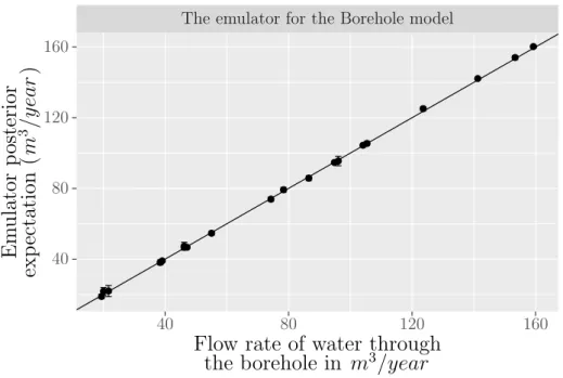
Before fitting a Gaussian process emulator, we transformed each input variables to be in the interval [−1,1]8. To construct the Gaussian process emulator with Bayesian framework, we assume that the prior uncertainty on the Borehole model is represented by a Gaussian process, equation (2.3.11). We used a linear mean function with h(x)T = (1,xT) and a covariance matrix, V = σ2C(x,x0), with the squared exponential correlation function C(x,x0) given in equation (2.3.4).
According to the training data, the parameters δ were estimated by the max-imum likelihood and the results are (0.64,10.34,5.69,0.64,3.72,0.28,5.73,0.43). It can be noticed that some inputs have large correlation length parameters, indi-cating that the simulator is more smooth with these inputs. After obtaining the estimated values of the parameters, the Gaussian process emulator was validated with 20 validation inputs, also generated by a SLHD, conditioned on the training points and the estimated correlation length parameters. Figure 2.3 shows the posterior emulator for the Borehole function with narrow 95% credible intervals. The predicted points seem to be reasonable since most of them lie on the y=x line. Moreover, the uncertainty, which is represented by the error bars, seems to be very small, indicating that the emulator predictions are good approximations of the simulator outputs with 95% credible intervals.
The emulator for the Borehole model 40 80 120 160 40 80 120 160
Flow rate of water through
the borehole in
m
3/year
Em
ulator
p
osterior
exp
ectation
(
m
3/y
ear
)
Figure 2.3: The posterior emulator approximations against observed values for the Borehole model with 95% credible intervals. The emulator predictions are good approximations of the simulator outputs with small 95% credible intervals.
2.7
Summary
In this chapter, we have reviewed the concept of emulators as surrogates of sim-ulators. We have presented the processes of building emulators based on the Bayesian perspective and we have presented some methods for estimating the Gaussian process parameters. We have shown how design points can be chosen using the Latin hypercube design and the sliced Latin hypercube design.
Since emulators have been used in various areas of science, it is necessary to check the validation of emulators before using them. In the next chapter, we review a number of diagnostic methods as well as develop a modification of an existing diagnostic method for validating Gaussian process emulators.
Chapter 3
Validating Gaussian process
emulators
3.1
Introduction
In this chapter, we explain the concept of uncertainty calibration in Gaussian process emulators. We also discuss situations where Gaussian process emulators may not perform well. We discuss the concept of diagnostics and review a number of published diagnostic methods for examining assumptions that are made in constructing Gaussian process emulators. We also develop a modification of an existing diagnostic method. Finally, we examine the performance of diagnostic methods with some different Gaussian process emulators in order to investigate whether these diagnostic methods can detect potential problems in some of these emulators.
3.2
Uncertainty calibration in emulators
In this section, we explain the concept of uncertainty calibration in Gaussian process emulators. When Gaussian process emulators do not perform well, we may obtain poor predictions of the simulator outputs or poor quantification of uncertainty in the emulator predictions. By poor predictions, we mean that the predictive mean is relatively far from the simulator outputs. By poor quantifi-cation of uncertainty, we mean the predictive variance is t
![Figure 2.1 shows a LHD of size 10 in the region χ = [0, 1] 2 . It can be seen that the marginal spaces of both input variables are well covered.](https://thumb-us.123doks.com/thumbv2/123dok_us/356717.2539253/43.892.197.706.285.647/figure-shows-region-marginal-spaces-input-variables-covered.webp)