Association Rules Mining Using Heavy Itemsets
Girish K. Palshikar
Tata Research Development and Design Centre (TRDDC), 54B, Hadapsar Industrial Estate,
Pune 411013, India. Tel.:91 20 4042500
email: [email protected]
Mandar S. Kale
Tata Consultancy Services (TCS), 54B, Hadapsar Industrial Estate,
Pune 411013, India. Tel.:91 20 4042469
email: [email protected]
Manoj M. Apte
Tata Consultancy Services (TCS), 54B, Hadapsar Industrial Estate,
Pune 411013, India. Tel.:91 20 4042471
email: [email protected]
ABSTRACT
A well-known problem that limits the practical usage of association rule mining algorithms is the extremely large number of rules generated. Such a large number of rules makes the algorithms inefficient and makes it difficult for the end users to comprehend the discovered rules. We present the concept of a
heavy itemset. An itemset A is heavy (for given support and
confidence values) if all possible association rules made up of items only in A are present. We prove a simple necessary and sufficient condition for an itemset to be heavy. We present a formula for the number of possible rules for a given heavy itemset, and show that a heavy itemset compactly represents an exponential number of association rules. We present an efficient greedy algorithm to generate a collection of disjoint heavy itemsets in a given transaction database. We then present a modified apriori algorithm that uses heavy items and detects more heavy itemsets, not necessarily disjoint with the given ones.
1. INTRODUCTION
Association rule mining, as originally proposed in [1] with its
apriori algorithm, has developed into an active research area.
Many additional algorithms have been proposed for association rule mining [2, 4, 7, 15]; see also [9]. Also, the concept of association rule has been generalized in many different ways, such as generalized association rules, association rules with item constraints, sequence rules [10] etc. Apart from the earlier analysis of market basket data, these algorithms have been widely used in many other practical applications such as customer profiling, analysis of products and so on. We have used these algorithms in innovative applications such as warranty claims analysis and inventory analysis. Several commercial data mining tools now offer variants of the association rule mining algorithms.
End users of association rule mining tools encounter several well-known problems in practice. First, the algorithms do not always return the results in a reasonable time. Typically, this happens
because the algorithms generate an exponential number of candidate frequent itemsets. Although several different strategies have been proposed to tackle efficiency issues, they are not always successful. Also, in many cases, the algorithms generate an extremely large number of association rules, often in thousands or even millions. Further, the association rules are sometimes very large. It is nearly impossible for the end users to comprehend or validate such large number of complex association rules, thereby limiting the usefulness of the data mining results. Several strategies have been proposed to reduce the number of association rules, such as generating only “interesting” rules, generating only “non-redundant” rules, or generating only those rules satisfying certain other criteria such as coverage, leverage, lift or strength. While these are promising strategies, none of them seem to sufficiently “compress” or reduce the generated association rules, for easy comprehension by end users.
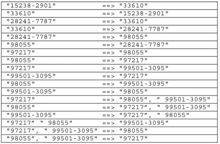
In this paper, we propose a concept called a heavy itemset. An itemset A is heavy (for given support and confidence values) if all possible association rules made up of items only in A are present. We prove a simple necessary and sufficient condition for an itemset to be heavy. We present a formula for the number of possible rules for a given heavy itemset, and show that a heavy itemset compactly represents an exponential number of association rules. We present an efficient greedy algorithm to generate a collection of disjoint heavy itemsets in a given transaction database. We then present a modified apriori algorithm that uses a given collection of heavy itemsets and detects more heavy itemsets, not necessarily disjoint with the given ones, and of course the remaining association rules. Table 1 shows an example, where the itemset {"97217”, “ 99501-3095", "98055"} is heavy (see last 12 rules).
The concept of heavy itemsets is useful in several practical applications; e.g., in a database of inventory or warranty claims, a group of parts (which forms an assembly) will often occur together. For example, when one assembly is replaced, all the member parts in that assembly are actually replaced. Either these relationships among the items will be known beforehand, or they will constitute an interesting new knowledge. (a) If we already know that some parts always occur together, then they can be modeled as heavy itemsets. In this case, the association rules among the member items of an assembly (which are already known) will be suppressed. This is particularly useful when the assembly consists of a large number of parts. (b) Discovering unknown heavy itemsets is a potentially interesting and useful ADVANCES IN DATA MANAGEMENT 2005
new knowledge. The algorithms presented in this paper can be used to discover only the heavy itemsets in a given transaction database,
The paper is organized as follows. Section 2 discusses some related work. The formal definition of the concept of heavy itemset and its theoretical properties are discussed in section 3. An efficient algorithm to generate a collection of disjoint heavy itemsets is presented in section 4. Section 5 contains the modified apriori algorithm, which uses a given collection of disjoint heavy itemsets as input, and generates “remaining” association rules and also finds more heavy itemsets, not necessarily disjoint from the given ones. Section 6 presents some experiments results. Section 7 presents conclusions and further work.
Table 1. Some association rules generated from real data. "15238-2901" ==> "33610"
"33610" ==> "15238-2901" "28241-7787" ==> "33610" "33610" ==> "28241-7787" "28241-7787" ==> "98055" "98055" ==> "28241-7787" "97217" ==> "98055" "98055" ==> "97217" "97217" ==> "99501-3095" "99501-3095" ==> "97217" "98055" ==> "99501-3095" "99501-3095" ==> "98055"
"97217" ==> "98055”, ” 99501-3095" "98055" ==> "97217”, “ 99501-3095" "99501-3095" ==> "97217”, “ 98055" "97217” “ 98055" ==> "99501-3095" "97217”, “ 99501-3095" ==> "98055" "98055”, “ 99501-3095" ==> "97217"
2. RELATED WORK
Association rule mining, as originally proposed in [1] with its
apriori algorithm, has developed into an active research area.
Many additional algorithms have been proposed for association rule mining [2, 4, 7, 15]; see also [9]. End users of association rule mining tools encounter several problems in practice, such as too much time taken by the algorithms and too many rules generated as output. Since finding support requires a pass over the entire database (and thus results in high I/O cost), one strategy to improve the efficiency involves the use of random sampling to estimate the support of an itemset; see [6, 13]. Use of hash-based efficient data structures [12] and mining of vertical (rather than horizontal) database [11] are some other approaches that have been tried to improve the efficiency of the association rule mining algorithms.
[16] compares 5 well-known association rule mining algorithms (viz., apriori, FP-tree, charm, Magnum-Opus and Closet) using 3 real-world data sets and observed super-exponential growth in the number of rules generated on these datasets. Several different strategies have been proposed to reduce the number of association rules generated. For example, we could use an interestingness measure to generate only interesting rules. See [5] for an excellent survey of many interestingness measures proposed in the literature. A closely related work is [14], which proposed the concept of a closed frequent itemset and used it to generate an
exponentially smaller number of non-redundant association rules. Several post-processing strategies have been proposed in [8] to reduce the number of generated association rules; e.g., prefer general association rules over specific ones, summarize and report only direction-setting (i.e., rules which indicate the type of correlation between specific itemsets) rules etc. In [3], algorithms are given to find itemsets containing highly correlated items i.e., association rules having high confidence but not constrained by any minimum support.
3. HEAVY ITEMSET
When generating association rules over a set of items, we often find that all possible association rules over a subset A of items are generated. Each of these association rules over A has the form X
Y where X and Y are disjoint non-empty subsets of A. These
rules clutter the generated output. They can be actually summarized (and hence removed from the output) by stating that
A is a heavy itemset.
Definition 1. Let L and R be any two non-empty disjoint itemsets.
Let 0.0 <σ,τ≤100.0 be the given support and confidence values. We say that LR is a valid association rule (for givenσandτ) if (i) support(L)≥ σand (ii) support(L∪R)≥ σand (iii) [support(L
∪R) / support(L)]≥ τ.
Definition 2. Let 0.0 <σ, τ ≤ 100.0 be the given support and confidence values. A non-empty itemset A (|A|≥2) is said to be a
heavy itemset (for givenσandτ) if for every non-empty disjoint subsets X, Y of A, XY is a valid association rule (for givenσ andτ). An element of a heavy itemset is called a heavy item.
It is easy to see that a subset (of cardinality 2 or more) of a heavy itemset is itself a heavy itemset. This observation, along with the efficient condition for checking whether a given itemset is heavy or not (as proved below) leads to a straightforward application of the apriori algorithm for mining only heavy itemsets. In each step of apriori, instead of finding frequent itemsets, we find heavy itemsets. However, we run into the same difficulties of an exponential number of candidates, in case there exist heavy itemsets of large size in a given transaction database. Instead, we use special properties of the heavy itemsets and give below a polynomial time algorithm for generating disjoint heavy itemsets.
We first formalize the concept of heavy itemset, so as to facilitate counting of the rules a heavy itemset represents.
Definition 3. Given a non-empty finite set A = {a1, a2, …, an} of n ≥2 items. A 2-split (or simply, a split) of A is a tuple (X,Y) where X, Y are non-empty disjoint subsets of A (i.e., X, Y⊆A, X≠ ∅, Y
For example, let A = {a, b, c, d}. Then ({a},{b, d}) is a split of A and so are ({b}, {d}), ({d}, {b}) and ({b, c}, {a, d}). The complete split-set of B = {a, b, c} containing 12 splits is:
{({a}, {b}), ({a}, {c}), ({b}, {a}), ({b}, {c}), ({c}, {a}), ({c}, {b}), ({a}, {b, c}), ({b}, {a, c}), ({c}, {b, a}), ({a, b}, {c}), ({a, c}, {b}), ({b, c}, {a})}
Thus a split represents an association rule; e.g., the split ({a}, {b,
c}) stands for the association rule {a}{b, c}. Then an itemset
A is heavy if all the association rules in the complete split-set of A
are present with the required support and confidence.
Proposition 1. The size of the complete split set (i.e., the number
of all possible splits) for a given finite set A of size N is given by
n m N N
m m N
n m N
C
C
−= −
=
¦ ¦
1 1
Here, m and n denote the sizes of the LHS and RHS sets in a spilt. Proof: The termNCmdenotes the number of ways in which the m elements in the left hand side set can be selected out of the total N elements. The termN-mCn denotes the number of ways in which the n elements in the right hand side set can be selected out of the remaining N – m elements. Since both LHS and RHS need to be selected, we take the product of these two terms (rule of product). Since the number of element m varies from 1 to N and m varies from 1 to N – m, we take the summations over all possible values of m and n, to get the total number of splits sets (rule of sum). When m = N, we assume that the term0Cn= 0.
Thus, if N = 3 (e.g., A = {a, b, c}), the total number of all possible splits is3C1⋅ (2C2 +2C1) + 3C2 ⋅ (1C1) = 3⋅ 3 + 3⋅1 = 12, as
shown above. If N = 4, the total number of possible splits is:
4C
1⋅(3C3+3C2+3C1) +4C2⋅(2C2+2C1) +4C3⋅1C1= 4⋅(1+3+3)
+ 6⋅(1 + 2) + 4⋅1 = 28 + 18 + 4 = 50.
It is easy to provide an upper bound on the summation in Proposition 1. Each item in the itemset A has 3 choices for each split: either it appears in the left side or it appears in the right side or it does not appear in either side. Thus the total number of possible rules for an itemset A of size n is bounded above by 3n. Since neither the RHS nor the LHS of an association rule can be empty, we need to eliminate such association rules. The number of association rules where the RHS is empty and the LHS is any subset of the itemset is 2n. Similarly, the number of association
rules where LHS is empty is also 2n. Since the empty association rule (LHS = RHS =∅) is counted twice, an alternative expression for the number of association rules corresponding to a heavy itemset of n items: 3n– 2n+1+ 1. This expression is equivalent to the one in Proposition 1.
Corollary 2: A heavy itemset compactly represents an
exponential number of association rules.
Proof: Immediately follows from the expression 3n– 2n+1+ 1.
We now prove a simple necessary and sufficient condition to decide whether an itemset is heavy or not.
Proposition 3: Suppose H = {a1, a2, …, an} is an itemset of n≥2
items. Let s0be the support of H. Let s1, s2, …, snbe the supports
of the singleton itemsets {a1}, {a2}, …, {an} respectively. Let the
minimum required support and confidence beσandτ. Let mn = min {s0, s1, s2, …, sn} and mx = max {s0, s1, s2, …, sn} be the
minimum and maximum of the support values. Then H is a heavy itemset iff (i) mn≥ σand (ii) (mn / mx)≥ τ.
Proof: (only-if part) Assume that (i) mn≥ σand (ii) (mn / mx)≥ τ.
H is a heavy itemset iff LR is a valid association rule for any
disjoint non-empty subsets L and R of H. Let L and R be any two disjoint non-empty subsets of H. We need to prove that (i) support(L)≥ σand (ii) support(L∪R)≥ σand (iii) [support(L∪
R) / support(L)]≥ τ. Clearly, support(L)≥mn. Given that mn≥ σ, it follows that support(L) ≥ σ. Similarly, we can prove that support(L ∪ R) ≥ σ. [support(L ∪ R) / support(L)] ≥ mn /
support(L)≥mn / mx which is given to be≥ τ; hence [support(L∪
R) / support(L)] ≥ τ as required. Hence L R is a valid
association rule. Since L, R are arbitrary disjoint subsets of H, we have proved that H is a heavy itemset.
(if part) Assume that H is a heavy itemset. We need to prove that (A) mn≥ σand (B) (mn / mx)≥ τ. Since mx = max {s0, s1, s2, …,
sn}, let L = {ak} be the singleton itemset such that support(L) = support({ak}) = mx. Let R = H \ L be the itemset of all items from
H except ak. Clearly, L, R are two disjoint subsets of H such that L
∪R = H and L∩R =∅. Then since H is a heavy itemset, LR
is a valid association rule. Hence, (i) support(L) ≥ σ and (ii) support(L∪R)≥ σand (iii) [support(L∪ R) / support(L)]≥ τ. Since support(L∪R) = s0= mn, it follows from (ii) that mn≥ σ,
thus proving (A) We now prove that (B) mn / mx≥ τ. In (iii), the numerator is the same as mn and the denominator is the same as
mx and hence it follows by substitution that mn / mx≥ τ.
We present below an algorithm that returns yes or no depending on whether or not the given itemset is heavy. Note that the algorithm uses the condition proved in Proposition 3 and does not explicitly check all the possible association rules to decide whether H is heavy or not.
algorithm is_heavy
input database D of N transactions
input heavy itemset H = {a1, a2, …, an} of n≥3 items
input minimum supportσ, minimum confidenceτ
output yes if H is a heavy itemset; no otherwise
1. Let s0be the support of H in D;
2. Let s1, s2, …, snbe the supports of {a1}, {a2}, …, {an} in D respectively;
3. Let mn = min {s0, s1, s2, …, sn} and mx = max {s0, s1, s2, …,
sn} be the minimum and maximum of the support values; 4. if mn <σthen return(no);
Correctness of the algorithm follows from Proposition 3. Checking this condition for a given itemset A requires one pass over the database to obtain support for each of the singleton subset of A and for A itself.
4. FINDING DISJOINT HEAVY ITEMSETS
4.1 FP-Tree
We first summarize the concept of the frequent-pattern tree, introduced in [4]. A frequent-pattern tree (FP-tree) consists of (i) a header, which is a sorted list of frequent itemsets in the descending order of their support (ii) vertices consisting of items in the header (iii) solid edge from an item u to item v having a link
count c if support of u≥support of v and u and v co-occur in c transactions (iv) dashed edge from each item u in the header to the first vertex in the tree for u (v) dashed edge from each vertex u to the next vertex for u in the tree. Thus, all the vertices in the tree for the same item u are ordered from left to right and connected into a sequence by dashed edges. Dashed edges do not have any count values. An FP-tree is a representation of all the transactions pruned to contain only items in its header. Support for an item u in the header is equal to the sum of the link counts of all solid edges that come into a vertex in the tree labeled with u. The algorithm for constructing an FP-tree is as follows. For simplicity, we omit the construction of the header of FP-tree, which contains frequent items in the given transaction database and their links.
algorithm build_fp_tree
input Transactions Database D
output FP-Tree T
1. Create a root node T of FP-Tree and label it as null. 2. do for every transaction t∈D
3. if t is not empty
4. insert (t, T)
5. link the new nodes to other nodes with similar labels links originating from header list.
6. return FP-Tree T
algorithm insert
input transaction t, any_node
1. do while t is not empty
2. if any_node has a child node with label head(t) then
3. increment link count between any_node and head(t) by 1 4. else create a new child node T0of any_node with label
head(t) and having link count 1
5. call insert(body(t), T0)
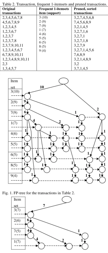
First column of Table 2 shows a database containing N = 12 transactions of 11 items. Forσ= 33%,τ= 33%, the 9 frequent 1-itemsets are shown in column 2 of Table 2. Column 3 of Table 2 shows each of the original transactions after (i) pruning the infrequent items (10, 11) and (ii) sorting the remaining items in the transaction in descending order of their support. Fig. 1 shows the FP-tree for these pruned and sorted transactions.
The path label for a path in an FP-tree is the minimum link count in that path; e.g., in Fig. 1, the path label of the path <root, 3, 2, 7, 1> is min{10, 9, 6, 4} = 4.
Table 2. Transaction, frequent 1-itemsets and pruned transactions.
Original transactions Frequent 1-itemsets item (support) Pruned, sorted transactions 2,3,4,5,6,7,8 4,5,6,7,8,9 1,2,3,4,5 1,2,3,6,7 1,2,3,7 1,2,3,7,8 2,3,7,9,10,11 1,2,3,4,5,6,7 6,7,8,9,10,11 1,2,3,4,8,9,10,11 2,3 1,3,4,5,7 3 (10) 2 (9) 7 (9) 1 (7) 4 (6) 5 (5) 6 (5) 8 (5) 9 (4) 3,2,7,4,5,6,8 7,4,5,6,8,9 3,2,1,4,5 3,2,7,1,6 3,2,7,1 3,2,7,1,8 3,2,7,9 3,2,7,1,4,5,6 7,6,8,9 3,2,1,4,8,9 3,2 3,7,1,4,5
Fig. 1. FP-tree for the transactions in Table 2.
Fig. 2. Conditional FP-tree for frequent item 1.
Given an item u in the header of an FP-tree T, we construct a new conditional FP-tree Tufor u as follows. Tuis the same as T except that it does not contain any vertex labeled with v (and solid edges incident on them) where v comes “after” u in the header of T or
root 3 Item set 3(10) 2(9) 7(9) 1(7) 4(6) 5(5) 6(5) 8(5) 9(4) 2 7 9 4 5 6 8 1 6 8 4 5 6 1 4 5 8 9 7 1 4 5 6 8 9 7 4 5 6 8 9 9 6 1 1 1 1 4 1 1 1 10 1 1 1 2 1 1
1 1 1
there is no path in T from the root to the vertex v which passes through u. The later condition essentially removes those transactions in which u is not present. Such items v are also removed from the header of Tu. The link counts in Tuand support values for items in the header are different from those in T; these are initialized to 0 and re-calculated as follows. Consider the frequent item 1; there are 3 paths <3,2,7,1>, <3,2,1>, <3,7,1> to the 3 vertices labeled 1 in the FP-tree T of Fig. 1. These paths represent a total of 7 transactions, since support(1) = 7 in the header of T. The path label for <3,2,7,1> is 4; so add 4 to each link count in this path. The path label for <3,2,1> is 2; so add 2 to each link count in this path. Finally, the path label for <3,7,1> is 1; so add 1 to each link count in this path. Now we find the new support for an item u in the header of Tu as the sum of the link counts of all solid edges that come into a vertex in the conditional FP-tree labeled with u. Fig. 2 shows the conditional FP-tree for frequent item 1.
4.2 Algorithm to Find Disjoint Heavy Itemsets
We now present an algorithm to find a collection of disjoint heavy itemsets for a given database D, supportσand confidenceτ.algorithm find_disjoint_heavy_itemsets input database D of N transactions.
input support , confidence
output a collection S of disjoint heavy itemsets 1. S =∅; h =∅; // h = current heavy itemset being built 2. (HD, T) = build_fp_tree(D) // HD is the header
3. nDepth = |HD|; // size of heavy itemset we are looking for
4. nHeavy = |HD|; // size of largest possible heavy itemset
5. while ( nDepth > 1)
6. if ( |h| > 0 ) // found heavy itemset h
7. S = S∪{h}; h =∅; // add h to S, re-init h to empty 8. delete all elements of h from HD
9. re-initialize all links in HD to NULL 10. nHeavy = nHeavy – |h|
11. nDepth = nHeavy
12. Delete the old FP-tree T
13. T = build_fp_tree(HD, D) // build new FP-tree
14. for every item I in HD do // start from last item
15. conditional_treeR(T, HD, I,σ,τ,∅, h) 16. nHeavy = nHeavy – 1
17. if nHeavy < nDepth then
18. break
19. nDepth = nDepth – 1
20. return S
algorithm conditional_treeR
input T, HD, I,σ,τ, nDepth // FP_tree,header,item,support,…
input L // list of items for which conditional tree is built
output h; // heavy itemset found
1. (HD1, T1) = build_conditional_fp_tree(T, HD, I)
2. Remove all elements of HD1 for which the support of the item (as per T1) in the element is <σ.
3. L = L∪{I}
4. CH = L∪HD1 // candidate heavy itemset
5. nHeavy = |CH|
6. if ( nHeavy < nDepth ) then
7. return 1 // don’t record this itemset on return path
8. if ( |HD1| > 1 ) then
9. if ( get_confidence(L) <τ) then
10. return 0
11. found = 0;
12. for every item I1∈HD1 such that I1≠I do
13. rec = conditional_treeR(T1,HD1,I1,σ,τ,nDepth,L,h)
14. if ( rec != 0 ) then found = 1;
15. nHeavy = nHeavy – 1
16. if ( nHeavy < nDepth ) then
17. return 1
18. if ( found = = 0 ) then
19. if (get_confidence(L) >τ) then {h = h∪L; return 1;}
20. else return 0;
21. return 1; // found something during recursion, so return 1 22. else // come here when |HD1|≤ 1
23. if (get_confidence(L) >τ) then { h = h∪CH; rec = 1; }
24. else rec = 0;
25. return rec
The subroutine build_fp_tree is the same as the one in [9]. The subroutine get_confidence computes the confidence of an itemset
A as per the formula 100 * (support(A) / mx), where mx = max
{support of elements of A}.
We now illustrate our algorithm for finding heavy itemsets. Initially, nDepth = nHeavy = 9, which is the number of frequent 1-itemsets. The subroutine conditional_treeR builds the conditional FP-tree T1 for item 9 and finds that there are no other items in the header HD1 of T1. The condition in line 6 is violated, the subroutine returns, nHeavy is decremented, condition in line 17 is violated, the for loop is exited. Thus there is no possibility of getting a heavy itemset of size 9. Hence nDepth is decremented and the algorithm starts looking for a heavy itemset of size 8. The algorithm continues and does not find any heavy itemsets of size upto 5 or more. Suppose nDepth = nHeavy = 4. The algorithm does not find any heavy itemset of size 4 for conditional FP-trees of items 9, 8, 6, 5, 4. Suppose now I = 1 in line 14 in find_disjoint_heavy_itemsets. We now enter the subroutine conditional_treeR and build the conditional FP-tree for 1 (Fig. 2).
5. THE apriori_heavy ALGORITHM
Suppose A is the set of all frequent 1-temsets in a given transaction database D. Suppose also that we find a collection H = {h1, h2, …, hk} of k heavy itemsets in D using the above algorithm. Let B be the set of all frequent items in A, which do not occur in any heavy itemset in S. Apart from the association rules consisting of items only in B, there may be additional association rules involving (i) relationships between items in different heavy itemsets in H; and (ii) relationships between items in B and items in one or more heavy itemsets in H. We now give an association rule mining algorithm, which uses H and B as given inputs and finds the set of all other “missing” association rules. The algorithm also finds more heavy itemsets, not necessarily disjoint from the given ones and adds them to H. Thus the generated collection of heavy itemsets H and the generated association rules complete the mining process.
algorithm apriori_heavy
input set of heavy itemsets H = {h1, h2, …, hk}
input set of frequent item B = {f1, f2, …, fm} where each {fi} is
a frequent 1-itemset and fi∉hj, for any hjin H
input transaction database D, supportσ, confidenceτ
ouput set of association rules LR
1. C2= {{u, v} | (∃1≤i, j≤k such that u∈hi∧v∈hj∧i≠j)
∨(∃1≤i≤m, 1≤j≤k such that u = fi∧v∈hj)
∨(∃1≤i ,j≤m such that i≠j∧u = fi∧v = fj) } 2. Find support of all 2-itemsets in C2to determine L2
3. move_to_heavy(L2,H) 4. k := 3; stop = 0;
5. while stop = 0 do
6. Ck= gen_candidate_itemsets(H,B,k,Lk-1)
7. prune(Ck,H,B)
8. Lk= set of all candidates in Ckhaving support≥ σ 9. if Lk=∅then stop = 1;
10. move_to_heavy(Lk,H) 11. k++
12. answer =∪Lk
algorithm move_to_heavy
input Lk, H // lists of frequent k-itemsets and heavy itemsets 1. for all itemsets l∈Lkdo
2. if is_heavy(l) then
3. H = H∪{l}
4. Remove all strict subsets of l from H 5. Lk= Lk– {l}
algorithm gen_candidate_itemsets
input set of heavy itemsets H = {h1, h2, …, hk}
input set of frequent item B = {f1, f2, …, fm} where each {fi} is
a frequent 1-itemset and fi∉hj, for any hjin H
input k, set Lk-1of frequent itemsets of size k-1 1. Ck=∅
2. for all itemsets l1∈Lk-1∪H such that |l1| = k-1 do
3. for all itemsets l2∈Lk-1∪H such that |l2| = k-1 do
4. if ( l1[1]=l2[1]∧l1[2]=l2[2]∧…∧l1[k – 1]<l2[k – 1] )
then
5. c = l1[1], l1[2], …, l1[k – 1], l2[k – 1]
6. if c⊄h’ for any h’∈H then Ck= Ck∪{c} 7. for all heavy itemsets h∈H do
8. for all itemsets l∈Lk-1∪H such that |l| = k-1 do 9. if (l does not contain any item from h) then
10. for all items i∈h do
11. c = l∪{i}
12. if c⊄h’ for any h’∈H then Ck= Ck∪{c} 13. else // l and h are not disjoint
14. let i0be the largest item of h present in l
15. for all items i∈h∧i > i0do
16. c = l∪{i}
17. if c⊄h’ for any h’∈H then Ck= Ck∪{c}
The algorithm apriori_heavy is nearly the same as the original
apriori algorithm, except for the following. The initial candidate
itemsets are of size 2, obtained by taking pair-wise Cartesian product of the heavy itemsets in H among themselves and with the set B of “non-heavy” frequent items. After finding the frequent k-itemsets, the algorithm checks (using subroutine is_heavy) if any of them are heavy itemsets; if so, then it removes that set from Lk and adds it to H, taking care to remove all proper subsets of the newly added heavy itemset from H. Since the set Lkmay become empty in this process, the terminating condition stated differently (stop when no new frequent itemsets are found).
In algorithm gen_candidate_itemsets, lines 2-7 are the nearly same as the original candidate generation scheme in apriori; except that heavy itemsets of size k-1 are also treated as frequent (k-1)-itemsets. Rest of the lines 7-17 pick a frequent (k-1)-itemset (or a (k-1) size heavy itemset from H) and systematically add one heavy element from H to it. The itemsets are assumed to be sorted as per the (arbitrary) item IDs.
A small modification is needed to actually generate the association rules from the resulting heavy itemsets and frequent itemsets. We omit the details here.
The trace of this algorithm on the database of Fig. 1 is as follows:
k = 2, H = {{1,2,3,7}, {4, 5}}, B = {6, 8, 9}
C2= {{1,4},{1,5},{1,6},{1,8},{1,9},{2,4},{2,5},{2,6},{2,8},
{2,9},{3,4},{3,5},{3,6},{3,8},{3,9},{4,6},{4,7},{4,8},{4,9}, {5,6},{5,7},{5,8},{5,9},{6,7},{6,8},{6,9},{7,8},{7,9},{8,9}}
L2= {{1,4},{2,4},{3,4},{3,5},{4,7},{5,7},{6,7},{7,8}}
We find that each itemsets in L2 is a heavy itemset; so we add
each of them to H. The new H is:
H = {{1,2,3,7},{4,5},{1,4},{2,4},{3,4},{3,5},{4,7},{5,7},{6,7},
{7,8}} L2=∅
k = 3
C3= {{3,4,5},{1,2,4},{1,3,4},{1,4,7},{1,4,5},{2,3,4},{2,4,7},
{2,4,5},{3,4,7},{3,5,7},{4,5,7},{4,6,7},{5,6,7},{4,7,8},{5,7,8}}
L3= {{3,4,5},{1,3,4},{2,3,4},{4,5,7}}
We find that each of these is again a heavy itemset; so we add them to H and delete all their subsets already in H. The new H is:
H = {{1,2,3,7},{3,4,5},{1,3,4},{2,3,4},{4,5,7},
{6,7},{7,8}} L3=∅
k = 4
C4= {{3,4,5,7},{1,3,4,7},{1,3,5,7},{2,3,4,7},{2,3,4,5}}
L4=∅
As an output of the algorithm apriori_heavy, we find the following heavy itemsets:
H = {{1,2,3,7},{3,4,5},{1,3,4},{2,3,4},{4,5,7},{6,7},{7,8}}
These itemsets altogether represent 50, 12, 12, 12, 12, 2, 2 association rules respectively. Note that some of the association rules “belong to” multiple heavy itemsets; e.g., 3 4 is represented by {3,4,5}, {1,3,4} and {2,3,4}. Any standard algorithm for association rule mining (e.g., apriori) reports 92 association rules for the example in Fig. 1 forσ= 33%,τ= 33%. We have “compactly represented” these 92 rules in terms of the 6 heavy itemsets, without loss of any information. Moreover, a heavy itemset represents a more meaningful relationship between the items, than in a single association rule.
There are no other rules left in this example, other than those represented by the heavy itemsets. However, in general, along with heavy itemsets, there would be other association rules as outputs of this algorithm. Note that the newly added heavy itemsets are not disjoint from one or more of the already known heavy itemsets {1,2,3,7} and {4, 5}.
As another example, for the following database of transactions,
1,3,5,6,8,9 1,2,5,7,9 2,3,5,6,7,9 1,2,5,6,8 2,3,4,5,7,9 3,4,6,8,9 2,3,5,7,8,9 1,2,4,5,6,7,9 1,2,3,6,8 1,2,3,5,7,9
we get the following heavy itemsets
3,9 2,5,7,9
and association rules (for support = 50% and confidence = 65%).
support,50.00,confidence,83.33,1,==>,5 support,50.00,confidence,83.33,1,==>,2 support,50.00,confidence,71.43,3,==>,5 support,50.00,confidence,71.43,3,==>,2 support,50.00,confidence,71.43,3,==>,5,9 support,50.00,confidence,100.00,3,5,==>,9 support,50.00,confidence,83.33,3,9,==>,5 support,50.00,confidence,71.43,5,9,==>,3
Note that any standard association rule mining algorithm will report 60 rules in the above transaction database (for these support and confidence values). But apriori_heavy reports only 8 association rules and 2 heavy itemsets. 50 association rules were suppressed because of the heavy itemset {2, 5, 7, 9} and 2 were suppressed because of the heavy itemset {3, 9}.
6. EXPERIMENTS
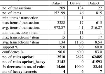
We have conducted several experiments on several real life data sets. We have observed considerable reduction in the number of
association rules generated by the apriori_heavy algorithm, as compared to the standard apriori algorithm. We present below some results. We have consistently seen considerable decrease in the number of association rules reported. This decrease is also dependent on the support and confident values used; e.g., for dataset-3, we observed a 100.0% decrease when the values support = 60.0% and confidence = 60.0% were used. We have also found that the facility of only identifying the heavy itemsets is of considerable use in practice.
Table 3. Experimental results.
Data-1 Data-2 Data-3
no. of transactions 209 134 22
no. of items 152199 46 815
min items / transaction 1 1 1
max items / transaction 3388 17 615 avg. items / transaction. 972.87 4.1 316.27
min transactions / item 1 11 1
max transactions / item 15 15 17 avg. transactions / item 1.34 11.96 8.54
support % 5.0 8.0 60.0
confidence % 90.0 60.0 83.0
no. of rules apriori 2510 2692 62485
no. of rules apriori_heavy 2142 0 41593
% decrease in no. of rules 14.66 100.0 33.44
no. of heavy itemsets 4 6 7
7. CONCLUSIONS AND FURTHER WORK
Most association rule mining algorithms suffer from the twin problems of too much execution time and generating too many association rules. In this paper, we proposed a solution to address the latter problem. We proposed the concept of heavy itemset, which compactly represents an exponential number of rules. We gave an efficient theoretical characterization of a heavy itemset. We presented an efficient greedy algorithm to generate a collection of disjoint heavy itemsets in a given transaction database. We then presented a modified apriori algorithm that uses given collection of heavy itemsets and detects more heavy itemsets, not necessarily disjoint with the given ones and of course the remaining association rules.We have implemented the algorithms proposed in this paper. The heavy itemsets are a useful and informative abstraction, which is clearly understood by the end users in business terms. Typically, a heavy itemset represents a group of items, which logically belong together; e.g., as a unit or assembly. We have tried the algorithms on several real life data sets and there is a drastic reduction in the number of generated association rules, due to the use of heavy items. Thus the end users can make better sense and use of the outputs of the association rule mining algorithms. The apriori_heavy algorithm usually shows a substantial improvement over the performance of the apriori algorithm, due to its use of heavy itemsets.
As further work, we are looking for a more efficient algorithm to generate all heavy itemsets, disjoint or not. We are also looking into a generalization of the heavy itemset that associates a degree
underlying association rules. For example, if a transaction database has all association rules (for a given support and confidence) of the form LR, where L⊆{a, b, c} and R⊆{p, q, r, s}, then all these rules can be compactly represented by stating that {a,b,c}{p, q, r, s} is a heavy association rule. Note that, in this case, {a,b,c,p,q,r,s} need not be a heavy itemset. Finally, we are investigating information theoretic characterization of the heavy items and heavy association rules.
8. ACKNOWLEDGMENTS
We thank Dr. Sachin Lodha for many constructive suggestions. Thanks also to Dr. Gautam Sardar for useful discussions. We sincerely thank Prof. Mathai Joseph for his support.
9. REFERENCES
[1] Agrawal R., T. Imielinski, A. Swami, “Mining Associations between Sets of Items in Massive Databases”, Proc. ACM
SIGMOD 1993, pp. 207-216.
[2] Brin S., R. Motwani, J. Ullman, S. Tsur, “Dynamic Itemset Counting and Implication Rules for Market Basket Data”,
Proc. ACM SIGMOD 1997.
[3] Cohen E., M. Datar, S. Fujiwara, A. Gionis, P. Indyk, R. Motwani, J. D. Ullman, C. Yang, “Finding Interesting Associations without Support Pruning”, Knowledge and
Data Engg., vol. 13, no. 1, 2001, pp. 64-78.
[4] Han, J., J. Pei, Y. Yin, “Mining Frequent Patterns without Candidate Generation”, Proc. ACM SIGMOD 2000.
[5] Hilderman R. J., H. J. Hamilton, “Knowledge Discovery and Interestingness Measures: A Survey”, Tech. Report CS-99-04, Dept. of Computer Science, Univ. of Regina.
[6] Karp R.M., S. Shenker, C. H. Papadimitrious, “A Simple Algorithm for Finding Frequent Elements in Streams and
Bags”, ACM Trans. Database Systems, Vol. 28, No. 1, March 2003, pp. 51-55.
[7] Lin D., Z. M. Kedem, “Pincer-Search: An Efficient Algorithm for Discovering the Maximum Frequent Set”,
IEEE Tran. Know. and Data Engg., Vol. 14, No. 3,
May/June 2002, pp. 553-556.
[8] Liu, B., W. Hsu, Y. Ma, “Pruning and Summarizing the Discovered Associations”, Proc. Fifth ACM-SIGKDD 1999, New York, pp. 125-134.
[9] Pujari A.K., Data Mining Techniques, University Press, 2001.
[10]Ramaswamy S., S. Mahajan, A. Silberschatz, “On the Discovery of Interesting Patterns in Association Rules”,
Proc. 24thVLDB Conf., 1998.
[11]Shenoy P., J. R. Haritsa, S. Sudarshan, G. Bhalotia, M. Bawa, D. Shah, “Turbo-charging Vertical Mining of Large Databases”, Proc. ACM SIGMOD 2000.
[12]Soo P. J., C. Ming-Syan, P. S. Yu, “Using a Hash-based Method with Transaction Trimming for Mining Association Rules”, IEEE Trans. Knowledge and Data Engg.,, Vol. 9, No. 5, Sep./Oct. 1997, pp. 813-825.
[13]H. Tiovonen, “Sampling Large Databases for Association Rules”, Proc. VLDB 2000.
[14]Zaki M. J., “Generating non-redundant Association Rules”,
Proc. KDD-2000, pp. 34-43.
[15]Zaki M. J., C. Hsiao, “Charm: An Efficient Algorithm for Closed Itemset Mining”, Proc. SIAM International
Conference on Data Mining, 2002.