*Corresponding author, Tel: +989132027395
Model Predictive Control and Stability Analysis
of a Standing Biped with Toe-Joint
Ehsan Kouchaki
a,*and Mohammad Jafar Sadigh
b aDepartment of Mechanical Engineering, Lenjan branch, Islamic Azad University, Isfahan, Iran, E-mail address: [email protected]. b
Department of Mechanical Engineering, Isfahan University of Technology, Isfahan, Iran
A R T I C L E I N F O A B S T R A C T
Article history:
Received: December 28, 2014. Received in revised form: April 21, 2015.
Accepted: May 1, 2015.
Keywords:
Model predictive control Toe-joint
Standing balance control Lyapunov exponents
In this paper standing balance control of a biped with toe-joint is presented. The model consists of an inverted pendulum as the upper body and the foot contains toe-joint. The biped is actuated by two torques at ankle-joint and toe-joint to regulate the upper body in upright position. To model the interaction between foot and the ground, configuration constraints are defined and utilized. To stabilize the biped around upright position, model predictive control (MPC) is implemented by which the constraints can be incorporate to the optimal control algorithm properly. To assess stability of system and to find domain of attraction of the fixed point, concept of Lyapunov exponents is utilized. Using the proposed control and stability analysis, we studied the effect of toe-joint in improving the stability of the biped and in decreasing actuator demand, necessary for stabilizing the system. In addition, effect of toe-joint is studied in improving domain of attraction of the stabilized fixed pint.
1. Introduction
The introduction section comes here. This document provides instructions for style. This document is a template for Microsoft Word. If you are reading a paper version of this document. The instructions are designed for the preparation of a regular paper and accepted Standing balance maintenance against unexpected external forces is one of the key requirements of bipedal robots operating in human environments. According to Investigations [1] one or a combination of two strategies namely ankle strategy and hip strategy are used by standing subjects (humans or bipeds) to keep their posture against disturbances. In the ankle strategy, the subject fixes all joints except the ankle and balances itself like a single inverted pendulum. Hip strategy on the other hand is characterized by a bending at the hip joint, which is used for large disturbances. Several control approaches based on aforementioned strategies have been developed such as optimal control [2], [3], ground reaction force feedback control [4], integral control [5], sensory adaption [6], biomechanically motivated strategy [7] and switching control based on foot-ground
constraints [8].
In the balanced standing state, the upper body situated in its upright position and the feet lie on the ground stationary. An important issue in this situation is the interaction between feet and the ground. During standing, the feet must be considered stationary but not fixed to the ground. That means there are constraints between the feet and the ground, which are essential and need to be satisfied for balanced standing.
not been addressed in the literature. In this paper we implement configuration constraints to our model to keep foot in contact with the ground during balance regulation.
All the previous work about bipedal standing balance control have used models with flat feet. A main limitation of them is the absence of toe-joints in their feet models. To the best of our knowledge, there is no work in literature dealing with the balance control of bipeds which contain toe-joints. Future bipedal robots are expected to be physically more interactive with their surroundings. Among this toe-joint plays a significant role to achieve more natural movements. It has been demonstrated that toe-joint led to higher stability [11], faster and smoother walking [12], better distribution of ground reaction forces [13] and lower energy consumption [14], [15].
In this paper we aim to present an optimal control algorithm for standing balance regulation of a bipedal model having toe-joint. The stabilization is done based on assumption of external disturbances to be small. Accordingly a simple bipedal model contains an inverted pendulum as the upper body and a foot with toe-joint is presented. To solve for stable configuration, one has to find fixed points of equations of motion which in case of foot with toe-joint leads to a set of undetermined equations. To overcome this problem, the interaction with the ground is supposed to be elastic. Controller for the system is designed using model predictive control (MPC) which provides an effective tool to handle constraints online in the optimal control algorithm. To evaluate the present model and investigate the effect of toe-joint, the results are compared with those of flat foot model without toe-joint in literature [8].
Although it is well known that such designed control makes the linearized model globally asymptotically stable, this will not be the case for the real nonlinear system. To assess stability of the nonlinear system around its fixed point to find domain of attraction of the fixed point, we used concept of Lyapunov exponents.
This paper consists of six sections. Equations of motion and constraints are presented in second section. The third section describes MPC formulation for control strategy. Stability analysis for nonlinear system is described in fourth section. The simulation results are given in fifth section followed by conclusions in the last section.
2. Modeling, equations of motion and constraints
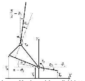
The bipedal model consists of an inverted pendulum represents the upper body and a foot which is composed of a heel-link and a toe-link. The biped is assumed laterally symmetric and moves in a sagittal plane. The model with its geometrical details is shown in Fig. 1. In the figure, and are toe length and heel length respectively. and
ℎ are horizontal and vertical distance between toe-joint and ankle. r is distance between the center of mass of the upper body and the ankle and L is the total length of
pendulum.
Fig 1. The biped model containing a toe-joint and an inverted pendulum as the upper body
Inverted pendulum models have often been used to study the bipedal posture. It has been reported in literature that when standing human subjects are perturbed by small disturbances in the sagittal plane from their upright position, they tend to keep the knees, hips and necks straight and moving about the ankle to keep balance (the ankle strategy) [1]. In this paper, small disturbances are considered. Thus, it is reasonable to simplify the upper body as an inverted pendulum.
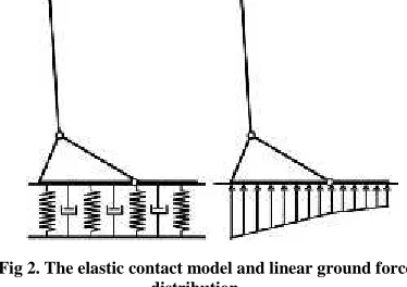
In the balancing state both heel and toe lie on the ground stationary. The resultant ground reaction force in this situation contains two forces acting on heel and toe. Evaluation of these forces and their lines of action leads to statically undetermined equations. To deal with this problem the contact between the foot and the ground is considered elastic in this paper. By this, the pressure distribution under heel and toe will get a linear form. Fig. 2 shows this elastic contact model and the consequent linear pressure distribution.
Fig 2. The elastic contact model and linear ground force distribution
Fig 3. The degrees of freedom and the applied joint torques In Fig. 3 and are the ankle torque and the toe-joint torque, respectively. , and are respectively the location of toe-joint, heel’s end and tip of the toe from level
ground (free length of the elastic support). is the angle of the toe-link with respect to the horizontal line (axes X) in the clockwise direction, is the angle between the toe-link and the heel and is the angle between the heel and the upper body. , and are respectively the absolute angles of the toe-link, the heel and the pendulum measured from the X axes in the positive trigonometrical direction.
The generalized coordinate of the system and the input torques are defined as follows:
= (1)
= (2)
The relations between the absolute and relative angles are:
= −
= − −
= 2 − − +
(3)
The potential energy due to deformation of the elastic support is obtained from:
P = k Y − x sin θ dx +
k Y + x sin θ dx (4)
where x is the path parameter from toe-joint along heel and toe-link and is the stiffness coefficient of the elastic support per length. The consumed power due to damping effects can be written as follows:
P = − k Y − x sin θ dx −
k Y + x sin θ dx
(5)
in which is the damping coefficient per length. The gravitational potential energy of the biped is obtained from:
P = m y g (6)
where g is the gravitational constant, is mass and is the vertical position of mass center of each link. The kinetic energy of the biped is:
= 12 + 12 (7)
where is the linear velocity of center of mass, is the angular velocity and is the mass moment of inertia of ith link. To obtain the equations of motion the terms of Eqs. 4-7 should be substituted in Lagrange equation:
− = + (8)
in which L is the Lagrangian and × is the Jacobian matrix:
= − − , =
0 0 0 0 1 0 0 1
(9)
The equations of motion were extracted using MATLAB and can be written in the following standard form:
M q q + h q, q = Du (10)
whereM × is the inertial matrix,h × is the centripetal, Coriolis and gravitational vector.
In this paper, the configuration constraints are used to model the interaction between the foot and the ground. Therefore, the foot should keep its contact with the ground during regulation. Since the foot consists of two rigid links, its overall position is defined by the location of end points i.e. as long as the end points of toe-link and heel (with position , and in Fig. 3) don’t rise from the ground
one can say the whole foot remains in contact with the ground. Accordingly, the configuration constraints can be expressed in terms of these points as:
≤ 0 ≤ 0
≤ 0 (11)
In Eq. 11,Y is one of the system’s degrees of freedom.
By rewriting and as functions of other degrees of freedom using Fig. 3 and Eq. 3, Eq. 11 becomes:
≤ 0
+ + ≤ 0
− ≤ 0
(12)
3. Standing balance control
The standing balance control is carried out using an optimal control rule based on model predictive control (MPC). Model predictive control is an effective strategy in which the constraints can be implemented online during the optimal control. The controller is designed based on the equations of linearized model around the equilibrium point. Since the stabilization against small disturbances with consequently small motions around the equilibrium configuration is studied in this paper, it is expected that the controller has a good performance. The design of controller is presented in this section.
Model predictive control (MPC) is an optimal control strategy based on the numerical optimization [16]. Future control inputs and future plant responses are predicted using a system model and optimized at regular intervals with respect to a performance index. Since MPC generally is implemented to the discrete form of motion equations, the discretization is done using zero-order hold method. The equations are:
+ 1 = + ( ) (13)
where A and B are state space matrices in discrete forms. x(k) and u(k) are the model state and input vectors at the kth sampling instant. Given a predicted input sequence, the corresponding sequence of state predictions is generated by simulating the model forward over the prediction horizon, of say N sampling intervals. These predicted sequences are stacked into following vectors:
=
| + 1|
⋮
+ − 1|
,
=
( + 1| ) ( + 2| )
⋮ ( + | )
(14)
Here u(k +i|k) and x(k +i|k) denote input and state vectors at time k +i that are predicted at time k. The predictive control feedback law is computed by minimizing a predicted performance cost, which is defined in terms of the predicted sequences U and X. and has the below quadratic form:
= ∑ + | + | +
+ | + | (15)
where Q and R are positive definite matrices (Q may be positive semi-definite). Clearly J(k) is a function of U(k) and the optimal input sequence for the problem of minimizing J(k) is denoted U*(k):
U∗ k = arg min j(k) (16)
Only the first element of the optimal predicted input sequence U*(k) is input to the plant:
= ∗ | (17)
The process of computing U*(k) by minimizing the predicted cost and implementing the first element of U* is then repeated at each sampling instant.
The preciseness of optimization depends on the length of prediction horizon N. The exact optimization occurs when J(k) is calculated in infinite horizon. Alternatively one can determine J(k) in a finite horizon by adding a terminal term to compensate the produced error. By doing this and using Eq. 14, index J(k) gets the following form:
J = U HU + 2 P U
+ G ( ) (18)
where;
H = C QC + R, P = C QM, G = M QM + Q, M
= A A … A
C =
B 0
AB B … 0… 0
⋮ ⋮
A B A B … B⋱ ⋮
, Q
= Q 0
0 Q … 0… 0
⋮ ⋮
0 0 … Q⋱ ⋮
, R
= R 0
0 R … 0… 0
⋮ ⋮
0 0 … R⋱ ⋮
Q × is the solution of Lyapunov equation. The
minimization of J(k) can be derived by letting gradient of J with respect to U to be zero:
∇ J = 2HU + 2P (19)
which leads to the below feedback law:
U∗ = − K ( ) (20)
whereK = H Pis the feedback gain matrix.
3.2. Incorporating constraints
To put the constraints into effect they should be applied to the optimization problem in each time step. To this end it is necessary first to write Eq. 12 in an appropriate matrix form in terms of states vector:
+ ( )
− ( ) ≤ 0 (21)
in which m1, m2 and m3 are following 8 × 8 matrices;
=
1 0
1 0 0 00 0 ×× 1 0
0 × 0 ×
0 0×
0 × 0 ×
=
0 0
0 1 0 01 0 ×× 0 0
0 × 0 ×
0 0 ×
0 × 0 ×
=
0 0
0 0 0 00 0 ×× 0 1
0 × 0 ×
0 0 ×
0 × 0 ×
By writing Eq. 21 in terms of predicted vector X(k) it gets the following form in the prediction space:
M X + sin M X( )
− sin M X( ) ≤ 0 (22)
where M1, M2 and M3 are 8N × 8N in which matrices m1, m2 and m3 are placed in their main diagonal N times respectively. The rest elements are zero. The minimization of J(k) with respect to constraints of Eq. 22 is a nonlinear programming problem because the constraints are nonlinear functions of predicted states vectors.
4. Stability analysis
In this section, stability of the system is investigated and the stability region is calculated in the phase plan using
effective tool, which is widely used for stability analysis of nonlinear systems, but in almost all cases, it is difficult to derive a Lyapunov function for highly nonlinear systems. Alternatively, Lyapunov exponents that are defined as the average exponential rates of divergence or convergence of nearby orbits in the state space [17], can characterize the system stability. The concept of Lyapunov exponents was employed for stability analysis of a flat foot biped before [8], [18]. In this section, the stability analysis of the current model is done using this concept.
Given the system’s equations of motion in the following
form with initial conditions:
= , , = (23)
When monitoring the long-term evolution of an infinitesimal n-sphere (n = 8) of initial conditions, the sphere will become an n-ellipsoid ball. The ith one-dimensional Lyapunov exponent is then defined in terms of the length of the ellipsoidal principal axis‖ ‖:
λ = lim→ 1 ‖‖ ( )‖( )‖ (24)
where are ordered from largest to smallest.‖ ‖ and‖ ‖denote the lengths of the ith principal axis of the infinitesimal 8-dimensional hyper-ellipsoid at final and initial times t and t0 respectively. The above definition of Lyapunov exponents indicate that Lyapunov exponents have a negative sign for stable systems and positive Lyapunov exponents represent the instability.
Since the ball of states establishes on a point of trajectory x with a small radius in each instance, the linearized model of Eq. 23 around each point of x is used for calculation of their evolution. By linearization around trajectory x the equations will get the following form:
δ = ∂ ,
∂ δ +
∂ ,
∂ δ (25)
By considering the states as direction axis, ∂ in the above equation is a matrix containing principal axis of the ball:
× = … (26)
Solving Eq. 25 with initial condition δ (0), the principal axis of ball will be obtained in each time step. The center of ball on the other hand moves on the trajectory x(t) generated by solving Eq. 23. Accordingly to assess the evolution of the ball, solving of Eqs. 23 and 25 is required simultaneously. This leads to the following set of equations:
δ =
,
∂ ,
∂ δ +
∂ ,
∂ δ
,
(0)
δ (0) = ×
(27)
where × is the identity matrix. By solving the above equations, the evolution of n-sphere spanned by δ is calculated. In order to avoid a misalignment of all the vectors along the direction of maximal expansion, Gram Schmidt reorthonormalization (GSR) is applied. GSR
provides the following orthonormal set:
= ‖ ‖, = ‖ ‖ ⋮
= ‖ ‖
(28)
in which , , … are defined as follows:
=
= − .
⋮
= − . …
− .
(29)
where < . > signifies the inner product. By solving the equations and using GSR procedure until K time step and step size T, the 8 Lyapunov exponents can be calculated from the below equation:
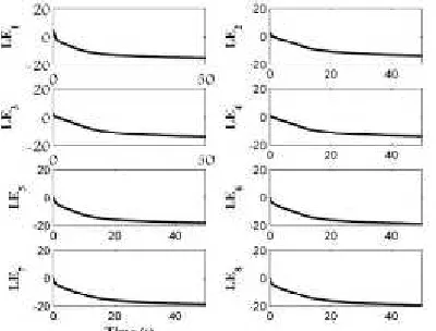
= 1 ‖ ( )‖ ( = 1, … ,8) (30)
5. Simulation results
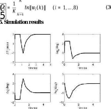
Fig 4. Simulated displacements in response to the initial angular velocity ( | = − . / )
In this section, simulation results are provided using numerical parameters. To be able to compare the results with those of flat feet, the numerical values of the physical parameters are adopted from literature [9] with additional parameters for the toe-link, as given in Table 1.
Table 1. Physical parameters used in the numerical simulation
Body height H = 1.78 m
Body mass mass = 80 kg
Heel mass mh = 1.46 kg
Toe mass mt = 0.86 kg
First, the equations of motion are linearized around the equilibrium points. The equilibrium points are calculated by letting the derivatives of the degrees of freedom be equal to zero in Eq. (10). Doing this the equilibrium points are obtained as a function of the applied torques:
= ̅ , ̅ = 1,2,3,4 (31)
where ̅ and ̅ are the static torques of toe-joint and ankle-joint in the equilibrium state. By solving the equations, several equilibrium points are obtained for each set of ̅ and ̅ . Among them, we choose one that gives biped the standing physical configuration in which the whole foot remains in contact with the ground and the upper body is upright. In this state static torques are zero ( ̅ = 0, ̅ = 0). The equilibrium position is calculated as (Yte = −0:011mm;q0e = 0:13o; qte = −1:23o; qae = −1:13o) which meansthat the upper body is upright ( =
90 ) and the whole foot is in contact with the ground. The simulation of standing balance control for numerical values of table 1 was done. The results are shown in Figs. 4-7 for primary five seconds in response to an initial angular velocity applied from back to the upper body ( | = − 0.6 / ). All other states are at their equilibrium values at the beginning. Fig. 4 shows the variation of states around the equilibrium point. The horizontal axis is simulation time and the vertical axis is the toe-joint displacement in the first plot and the angular displacements of other degrees of freedom in the three rest plots. From Fig. 4 one can see that the controller works properly and biped is stabilized to its equilibrium situation within 3 seconds.
Fig 5. Displacement of foot points: : toe-joint, : heel end, : toe end
Fig. 5 shows simulated vertical displacements of end points of foot links namely toe-joint, heel end and tip of the toe. As shown in the figure the curves go to the equilibrium status within 3 seconds. Note that the saturated parts of plots that appear as cut curves in the zero position of vertical axis (ground level) in some instants of simulation time are due to the implementation of configuration constraints that restrict the biped to keep the whole foot in contact with the ground during regulation
Fig. 6 shows the history of torques applied from controller within simulation time. The dash curve is
ankle’s torque and the dash-dot one is toe-joint’s torque.
The solid line is control torque of previous work [8], which is added for comparison. In that work a flat foot biped without toe-joint and with the same physical parameters was studied and the standing balance control was done using a state-switching PD controller. Note that the initial conditions of two models are same. As it seen, the control torque applied by ankle’s actuator has been reduced
significantly due to contribution of toe-joint. Furthermore, figure shows that the total amount of control torques of the present model is lower than that of toe-less model.
Fig 6. Simulated control torques: the flat foot model [8]:-, : -., :
-In Fig. 7 the variation of the upper body angular displacement with respect to vertical line is shown. The dash curve is for the present model and the solid one is for the flat foot model [8]. The figure shows that both controllers stabilize the biped within 3 seconds. However the present control system has a better performance.
Eight Lyapunov exponents for the control system were calculated. It was observed that for the system after 50 seconds all Lyapunov exponents converge to certain values. In Fig. 8 Lyapunov exponents are shown with respect to time for 100 seconds with the converged values mentioned in the caption. All Lyapunov exponents converged to negative values so the control system is stable for that initial conditions.
-Fig 8. Lyapunov exponents of the control system converged to: LE1 = 13:78; LE2 = 13:79; LE3 = 14:05;LE4 = 15:44;LE5 =
-18:08;LE6 = -18:615;LE7 = -18:8;LE8 = -19:19
Since Lyapunov exponents remain negative values within the stability region, the determination of the stability region becomes an important part of the stability analysis. Since the angular displacement and velocity of the upper body are key states, and the purpose of control was the regulation of upper body to the upright position the calculation of stability region was done in the phase plane
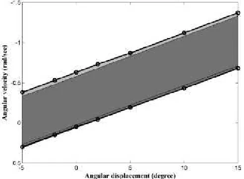
, To determine the stability region, Lyapunov exponents were determined by taking neighborhood points of the origin in the phase plane as initial conditions. The stability region is the area in the phase plane in which the taken initial conditions lead to converged Lyapunov exponents. Fig. 9 shows the resultant stability region in light gray. The horizontal axis is angular displacement of the upper body and the vertical axis is its angular velocity. The stability region of the flat feet model without toe-joints calculated in the previous work [9] is added in dark gray for comparison. The figure shows that the present model gives a wider stability region.
Fig 9. Stability region determined by Lyapunov exponents: present model: gray region, toe-less model [9]: black region
6. Conclusions
In this paper, standing balance control for a biped with toe-joint was presented. The bipedal model contained an inverted pendulum as the upper body and a toe-joint in its foot. The biped was actuated in both ankle and toe-joints. Configuration constraints between foot and ground were defined to keep the foot in contact with the ground during balance regulation. The regulation of upper body around upright position was done using model predictive control. The stability of system was analyzed using concept of Lyapunov exponents.
The main contribution of this work is modeling the toe-joint in standing balance control and applying configuration constraints during regulation, which have not been addressed so far. Simulation results showed that the designed controller could stabilize the biped properly. Compared with the flat foot bipedal model studied in the literature, the present model with toe-joint showed a better performance and the controller demanded lower control torques for regulation. Furthermore, the stability region of this model was greater than those of toe-less model.
References
[1] F. Horak and L. Nashner, Central programming of postural movements: adaptation to altered support-surface configurations, Journal of Neurophysiology, Vol. 55(6), (1986), 1369-1381
[2] A.D. Kuo, An optimal control model for analyzing human postural balance, IEEE Transaction Biomedical Engineering, Vol. 42, (1986), 87-101.
[3] C. Liu and C.G. Atkeson, Standing balance control using a trajectory library, IEEE/RSJ Int. Conf. on intelligent robots and systems, Louis, USA, (2009), 3031-3036.
[4] S. Ito, H. Takishita and M. Sasaki, A study of biped balance control using proportional feedback of ground reaction forces, SISE-ICASE. International Joint Conference, Bexco, Busan, Korea, (2006), 2368-2371. [5] B. Stephens, Integral Control of Humanoid Balance, The International Conference on Intelligent Robots and
Systems (IROS’07), San Diego, CA, (2007).
[6] A. Mahboobin, P. J. Loughlin, M. S. Redfern, S. O. Anderson, C. G. Atkeson, Sensory adaptation human balance control: Lessons for biomimetic robotic bipeds, School of computer science, Carnegie Mellon University, (2008).
[7] M. Abdallah and A. Goswami, A biomechanically motivated two-phase strategy for biped upright balance control, IEEE Int. Conf. on robotics and automation, Barcelona, Spain, (2005), 2008-2013.
[8] C. Yang and Q. Wu, On stabilization of bipedal robots during disturbed standing using the concept of Lyapunov exponents, Robotica, 24(5), (2006), 621-624.
bipedal balance control during standing, Int. J. Humanoid Robotics, 4, (2007), 753-775.
[10] E. Kouchaki, Q. Wu and M. J. Sadigh, Effects of constraints on standing balance control of a bipeds with toe-joints, International Journal of Humanoid Robotics, 9(3), (2012).
[11] C. K. Ahn, M. C. Lee and S. J. Go, Development of a biped robot with toes to improve gait pattern, IEEE/ASME Int. Conference on Advanced Intelligent Mechatronics, (2003), 729-734.
[12] R. Sellauoti and O. Stasse, Faster and Smoother Walking of humanoid HRP-2 with passive toe-joints, IEEE/RSJ Int. Conf. on Intelligent Robots and Systems, Beijing, China, (2006), 4909-4914.
[13] K. Yamamoto and T. Sugihara, Toe-joint mechanism using parallel four-bar linkage enabling humanlike multiple support at toe pad and toe tip, Int. Conf. on Humanoid Robots, Pittsburgh, USA, (2007), 410-415. [14] D. Tlalolini, C. Chevallereau, and Y. Aoustin,
Human-like walking: optimal motion of a bipedal robot with toe-rotation motion, IEEE/ASME Transactions on Mechatronics, 16, (2011), 310-320.
[15] E. Kouchaki, M.J. Sadigh, Effect of Toe-Joint Bending on Biped Gait Performance, IEEE Int. Conf. on robotics and biomimetics, Tianjin, China, (2010), 697-702.
[16] M. Cannon, Model predictive control, Lecture notes, Oxford University, (2011).
[17] A. Wolf, J. B. Swift, H. L. Swinney, and J. A. Vastano, Determining Lyapunov Exponents from a Time Series, Physics D, 16, (1985), 285317, 1985. [18] C. Yang, Q. Wu, On stability analysis via Lyapunov
exponents calculated from a time series using nonlinear mapping-a case study, Nonlinear Dynamics, Vol. 59, (2010), 239-257.
Ehsan Kouchaki received his B.Sc., M.Sc. and Ph.D. degrees in Mechanical Engineering from Isfahan University of Technology, Iran, in 2003, 2006 and 2013, respectively. He is currently a faculty member of mechanical engineering at Lenjan branch, Islamic Azad University, Iran. His research interests include robotics, control and nonlinear dynamics.