Nordsieck representation of high order predictor-corrector Obreshkov methods and their implementation

(1)

Nordsieck representation of high order predictor-corrector Obreshkov

methods and their implementation

Behnaz Talebi

Faculty of Mathematical Sciences, University of Tabriz, Tabriz, Iran. E-mail: [email protected]

Ali Abdi∗

Faculty of Mathematical Sciences, University of Tabriz, Tabriz, Iran. E-mail: a [email protected]

Abstract Predictor-corrector (PC) methods for the numerical solution of stiﬀ ODEs can be extended to include the second derivative of the solution. In this paper, we con-sider second derivative PC methods with the three-step second derivative Adams-Bashforth as predictor and two-step second derivative Adams-Moulton as corrector which both methods have order six. Implementation of the proposed PC method is discussed by providing Nordsieck representation of the method and preparing an starting procedure, an estimate for local truncation error and a formula for chang-ing stepsize. Eﬃciency and capability of the method are shown by some numerical experiments.

Keywords. PEC methods, Adams methods, Nordsieck representation, Local error estimation, Variable

stepsize.

2010 Mathematics Subject Classification. 65L05.

1. _Introduction

Many codes have been introduced for solving

y′(x) =f(x, y), y(x0) =y0, x∈I:= [x0, x], (1.1)

where f : I×Rm → Rm and m is the dimensionality of the system, in the class of linear multistep methods (LMMs) which use ﬁrst derivatives of the solution (for instance [6,9,15]). Adams methods [7,14] for the numerical integration of (1.1) are an special case of LMMs which are usually implemented in predictor-corrector (PC) form.

For problems in which

g(x, y) :=fx(x, y) +fy(x, y)·f(x, y) =y′′,

can be calculated along withf(x, y), at a moderate additional cost, second derivative methods become feasible which can be of high order of accuracy. In this class of the

Received: 13 November 2017 ; Accepted: 23 October 2018.

∗Corresponding author.

(2)

methods, some successful methods have been introduced that have good properties, especially for stiﬀ problems [1, 2, 3, 4, 5, 8, 10, 11, 12, 13, 16, 17]. Here, we will use second derivative Adams methods as PC pairs which k–step second derivative Adams-Bashforth method (ABM)

yn =yn₋1+h(ˆa1fn₋1+ ˆa2fn₋2+· · ·+ ˆakfn₋k)

+h2(ˆb1gn−1+ ˆb2gn−2+· · ·+ ˆbkgn−k),

(1.2)

is used for predicted part and (k−1)–step second derivative Adams-Moulton method (AMM)

yn =yn−1+h(a0fn+a1fn−1+· · ·+ak−1fn−k+1)

+h2(b0gn+b1gn−1+· · ·+bk−1gn−k+1),

(1.3)

is used for corrected part. Here, fn−i = f(xn−i, yn−i) and gn−i = g(xn−i, yn−i), i= 0,1, . . . , k.

In this paper, we describe a nice approach to the implementation of the PECE (predict-evaluate-correct-evaluate) mode of PC formulas (1.2)–(1.3) with k= 3 in a variable stepsize environment using Nordsieck representation. Fork= 3, the coeﬃ-cients of the methods (1.2) and (1.3) are chosen so that these methods have order six. In this way, the resulting ABM and AMM take the forms

yn =yn−1− 949

240hfn−1+ 38

15hfn−2+ 581

240hfn−3+ 637 240h

2_g

n−1

+9 2h

2_g

n−2+ 173 240h

2_g

n−3,

(1.4)

and

yn =yn−1+ 101 240hfn+

8

15hfn−1+ 11

240hfn−2− 13 240h

2_g

n

+1 6h

2_gn

−1+ 1 80h

2_gn

−2,

(1.5)

respectively.

The paper is organized along the following lines. In Section 2, Nordsieck represen-tation of the PC pairs (1.4) and (1.5) is obtained. This leads to a discussion of the variable stepsize mode of the proposed method and implementation issues including starting procedures, local error estimation and stepsize control. These are explained in Section 3. Finally, some numerical results are given in Section 4 to show eﬃciency of the method.

2. _{Nordsieck representation of the PC pairs}

(3)

For a Nordsieck method of orderp, the input and output data at the step number

nare in the form

Np,n−1=      

y(xn₋1)

hy′(xn₋1) .. .

hpy(p)(xn₋1)      +O(h

p+1_{) and} _N

p,n=      

y(xn)

hy′(xn) .. .

hpy(p)(xn)      +O(h

p+1₎_,

respectively. So, for our method which is of order six, the output vector must have seven components including values at the current pointxn and previous pointsxn₋1 andxn₋2. We choose the output vector as

Yn =

          yn hfn h2_gn

hfn₋1

h2_gn

−1

hfn₋2

h2gn₋2           =          

y(xn) hy′(xn) h2_y′′₍_xn₎

hy′(xn₋1)

h2_y′′₍_xn

−1)

hy′(xn₋2)

h2y′′(xn₋2)          

+O(h7). (2.1)

Wherey(x) is the exact solution of the equationy′=f(x, y) at the pointx. By using Taylor expansion for each component of the vector in the right hand side of (2.1), we have          

y(xn)

hy′(xn)

h2_y′′₍_xn₎

hy′(xn₋1)

h2y′′(xn₋1)

hy′(xn₋2)

h2y′′(xn₋2)           =T              

y(xn)

hy′(xn)

h2

2!y′′(xn)

h3

3!y′′′(xn)

h4

4!y (4)₍_x

n) h5

5!y (5)₍_x

n) h6

6!y (6)₍_xn₎

             

+O(h7), (2.2)

where T =          

1 0 0 0 0 0 0

0 1 0 0 0 0 0

0 0 2 0 0 0 0

0 1 −2 3 −4 5 −6

0 0 2 −6 12 −20 30

0 1 −4 12 −32 80 −192

0 0 2 −12 48 −160 480

          .

So, we obtain the relation between the vectorsYn andNn given by

Yn =T N6,n. (2.3)

(4)

• First stage

At the ﬁrst stage, we obtain an approximation using predictor equation

yn∗ =yn−1− 949

240hfn−1+ 38

15hfn−2+ 581

240hfn−3+ 637 240h 2_gn −1 +9 2h 2_gn

−2+ 173 240h

2_gn

−3.

(2.4)

Since the valuesyn₋1, fn−1, gn−1, fn−2, gn−2, fn−3, and gn−3 are available, the vector representing input and output data at the step numbern, are in the form

Zn−1≈          

y(xn−1)

hf(xn−1)

h2_g₍_x

n−1)

hf(xn−2)

h2_g₍_xn

−2)

hf(xn₋3)

h2_g₍_xn

−3)          

and Zn ≈

         

y(xn) hf(xn) h2_g₍_x

n) hf(xn−1)

h2_g₍_xn

−1)

hf(xn₋2)

h2_g₍_xn

−2)           , (2.5)

respectively. Now we deﬁne the vectorZ_n∗: The ﬁrst component of it is y_n∗

obtained by predictor equation (2.4) and the next two components are related to the evaluate step, and the last four components arehf(xn₋1),h2g(xn₋1),

hf(xn₋2), andh2g(xn₋2). So it can be written in the form

Z_n∗=H Zn₋1, (2.6)

where H=          

1 −949₂₄₀ 637₂₄₀ 38₁₅ 9₂ 581₂₄₀ 173₂₄₀

0 0 0 0 0 0 0

0 1 0 0 0 0 0

0 0 1 0 0 0 0

0 0 0 1 0 0 0

0 0 0 0 1 0 0

          .

We note thatZ_n∗ means the vector of predicted values andZn−1 is the vector of values at the previous step.

• Second step

The second step is to evaluate functionsf and g at the point (xn, y_n∗) and add them into the formula (2.6). To do this, we deﬁne the vectors

E1= [

0 hf(xn, y∗n) 0 0 0 0 0

]

,

and

E2= [

0 0 h2g(xn, yn∗) 0 0 0 0

]

,

then we deﬁne a new vector of two stages predict-evaluate in the form

(5)

To write (2.7) in terms of Nordsieck vectors, at ﬁrst we note that by Taylor expansion, we have

E1=e2 [

0 1 2 3 4 5 6]N6,n₋1+O(h7),

and

E2=e3 [

0 0 1 3 6 10 15]N6,n−1+O(h7),

where the vectorse2ande3 are the second and third columns of the identity matrix of dimension seven, respectively. Now, the Nordsieck representation of (2.7) is

N₆∗_,n=P N6,n−1,

with

P=T−1HT +T−1e2 [

0 1 2 3 4 5 6]

+ 2T−1e3 [

0 0 1 3 6 10 15],

which is the upper triangular Pascal matrix.

• Third step

In this step, we include the correction equation. The Nordsieck representation for PEC Adams method of order six is

N6,n=P N6,n−1+δ1T−1α+δ2T−1β, (2.8)

where α and β are equal to vectors a0e1+e2 and b0e1+e3, that are the corresponding coeﬃcients a0 = 101₂₄₀ and b0 = −₂₄₀13 from the terms 101₂₄₀hfn and−₂₄₀13h2_gn_{, respectively, in the correction equation (}_1.5_{). Here, the error} estimationsδ1 andδ2with

δ1=hf(y∗n)−[0 1 2 3 4 5 6]N6,n−1,

δ2=h2g(yn∗)−2[0 0 1 3 6 10 15]N6,n−1.

represent the correction of the ﬁrst and second derivatives, respectively.

• Fourth step

Finally, we include the ﬁnal step which is related to the functions evaluations at (xn, yn)

fn=f(xn, yn), gn=g(xn, yn),

to be used in the next time step.

3. _{Practical implementation of the method}

In this section, we concentrate on the implementation issues for our method. Nord-sieck PC method (2.8) in the variable stepsize mode is in the form

(6)

where

T1= [₁₀₁

240 1 0 −

23

12 −

33

16 −

17 20−

1 8 ]

,

T2= [

−13

240 0 1 2 1

13 16

3 10

1 24

]

.

andD(θn) is the rescaling matrix deﬁned by

D(θn) := diag(1, θn, θ2_n, . . . , θp_n),

withθn as the ratio of consecutive stepsizes,θn=hn/hn₋1, andhn=xn−xn−1.

3.1. Starting procedure. For the method of orderp= 6 (2.8), a starting procedure of order six is required to approximate the initial Nordsieck vectorN6,0 which is an approximation to the vector

[

y(x0) hy′(x0)

h2

2!y

′′₍_x

0) · · ·

h6

6!y (6)₍_x

0) ]T

.

Since the ﬁrst three components of this vector is known, we need to approximate only the last four components of that. To do that, we carry out one step of a Runge–Kutta method with abscissa vectorecwhich gives suﬃcient output information,ye1≈y(x0+

h0) andYie ≈y(x0+ecih0),i = 1,2, . . . , s. We can obtain a reliable approximations by using some linear combination of these information as

h3y(3)(x0) =a1y(x0) +a2hy′(x0) +a3h2y′′(x0) +a4h2g(eY1) +a5h2g(eY2)

+a6h2g(Ye3) +a7h2g(Ye4) +O(h7),

h4y(4)(x0) =b1y(x0) +b2hy′(x0) +b3h2y′′(x0) +b4h2g(Ye1) +b5h2g(Ye2)

+b6h2g(Ye3) +b7h2g(Ye4) +O(h7),

h5y(5)(x0) =c1y(x0) +c2hy′(x0) +c3h2y′′(x0) +c4h2g(Ye1) +c5h2g(Ye2)

+c6h2g(Ye3) +c7h2g(Ye4) +O(h7),

h6y(6)(x0) =d1y(x0) +d2hy′(x0) +d3h2y′′(x0) +d4h2g(Ye1) +d5h2g(Ye2)

+d6h2g(Ye3) +d7h2g(Ye4) +O(h7).

3.2. Local error estimation. The local truncation error of a method of orderp, in the step numbern, is deﬁned by

LTE(xn) =Cphp+1y(p+1)(xn) +O(hp+2),

where Cp is the error constant of the method. In order to control the stepsize, we need to estimate the local truncation error for each step. Here, the estimation of LTE is produced by using the Milne device which is based on the diﬀerence of the predictor and corrector approximations: Denoting the error constants for the Adams-Bashforth and Adams-Moulton of orderpbyC_p∗ andCp, respectively, we have

y∗_n=y(xn)−Cp∗h

p+1_y(p+1)₍_x

(7)

yn=y(xn)−Cphp+1y(p+1)(xn) +O(hp+2),

which using the Milne device implies

y(xn)−yn = Cp Cp−Cp∗

(y∗−yn) +O(hp+2).

Forp= 6, we haveC6∗= 53

4725,C6= 1

9450, and so

y(xn) =yn+

1

105(yn−y

∗

n) +O(h

8₎_.

Hence∥LTE(xn)∥can be estimated as

∥LTE(xn)∥=

1

105∥(yn−y

∗ n)∥.

3.3. Stepsize control. After estimating the local truncation error, we can control the stepsize by monitoring this estimation. For the given absolute and relative toler-ances,AtolandRtolrespectively, we use the following control

∥LTE(xn)∥ ≤Rtol·max{∥yn∥,∥yn+1∥}+Atol, (3.2) to control the stepsize in the proceeding fromxn to xn+1. If the control (3.2) is not satisﬁed, the current step is repeated with the halved stepsize. Otherwise, the current step is accepted and we carry our the next step with the new stepsize as

hn+1=θn+1hn,

where

θn+1= min {

2, α

( _tol

∥LTE(xn)∥

)1 7}

.

In our numerical experiments we have usedAtol=Rtol=tol, and the safety factor

α= 0.9 to guard against unnecessary step failures.

4. _{Numerical experiments}

In this section we present the results of numerical experiments to show eﬃciency of the constructed method of order six in the variable stepsize mode.

Computational experiments are done by applying our method on the following problems.

P1. The modiﬁed Kepler problem 

             

y′₁=∂H_∂y(y)

3 , y′₂=∂H_∂y(y)

4 , y′₃=−∂H_∂y(y)

1 , y′₄=−∂H_∂y(y)

(8)

withH(y) = y 2 3+y24

2 −

1

r − ϵ

2r3 andr= √

y2

1+y22 whereϵis a positive or negative small number. The initial conditions are

            

y1= 1−e,

y2= 0,

y3= 0,

y4= √

1 +e

1−e.

In the numerical results, we takeϵ= 0.01 ande= 0.6.

P2. The famous Lorenz equations provide a simple example of a chaotic system. They are given by

    

y′₁=σ(y2−y1),

y′₂=ry1−y2−y1y3,

y′₃=y1y2−by3,

where σ, r and b are positive parameters. Following Lorenz, we set σ = 10, b = 8/3, r= 28,y(0) = [0,1,0]T andx∈[0,50].

P3. The third problem is the Kepler’s problem also known as the one-body problem which describes the motion of a single planet moving around a heavy sun. The problem is given by

              

y′₁=y3,

y′₂=y4,

y′₃= −y1 (y2

1+y 2 2)3/2

,

y′₄= −y2 (y2

1+y 2 2)3/2

,

and the initial values are prescribed to be 

           

y1= 1−e,

y2= 0,

y3= 0,

y4= √

1 +e

1−e,

where e is the eccentricity of an ellipse on which the orbit lies. With these initial values, all points in the orbit lie on the ellipse

(y1+e)2+

y2 2 1−e2 = 1.

The results of numerical experiments for these problems are presented in Tables

(9)

Table 1. Numerical results for problem P1 solved by the method (3.1) withh0= 10−2andx∈[0,500].

tol ns nrs hmin hmax ge

10−10 ₉₇₈₇ ₁₈₅ _≈₆_.₉₂_×₁₀−4 _≈₂_.₁₁_×₁₀−1 ₆_.₈₁₃₆_×₁₀−12

10−11 ₁₃₃₆₅ ₅ _≈₃_.₂₇_×₁₀−4 _≈₁_.₄₈_×₁₀−1 ₆_.₄₀₃₇_×₁₀−12

10−12 ₁₈₅₈₃ ₆ _≈₁_.₅₆_×₁₀−4 _≈₁_.₀₄_×₁₀−1 ₅_.₈₃₆₇_×₁₀−13

10−14 35896 8 ≈3.64×10−5 ≈5.33×10−2 5.2873×10−15

Table 2. Numerical results for problem P2 solved by the method (3.1) withh0= 10−2andx∈[0,50].

10−7 ₄₉₅₂ ₅₉₂ _≈₁_.₃₂_×₁₀−3 _≈₂_.₆₅_×₁₀−2 ₃_.₇₂₃₇_×₁₀−8

10−8 5289 278 ≈6.47×10−4 ≈2.05×10−2 4.5766×10−9

10−9 6474 48 ≈3.05×10−4 ≈1.71×10−2 6.0246×10−10

10−10 ₈₉₂₃ ₉ _≈₁_.₄₆_×₁₀−4 _≈₁_.₂₆_×₁₀−2 ₄_.₇₈₃₈_×₁₀−11

Table 3. Numerical results for problem P3 solved by the method (3.1) withe= 0.5,h0= 10−3and x∈[0,10π].

10−10 759 331 ≈4.98×10−4 ≈1.85×10−1 1.6253×10−7

10−11 1050 488 ≈1.79×10−4 ≈1.14×10−1 1.0812×10−8

10−12 ₁₄₄₈ ₆₇₇ _≈₂_.₅₁_×₁₀−4 _≈₈_.₉₅_×₁₀−2 ₁_.₃₆₅₈_×₁₀−9

10−14 ₂₇₇₈ ₁₃₁₃ _≈₄_.₈₇_×₁₀−5 _≈₅_.₀₇_×₁₀−2 ₁_.₃₁₆₆_×₁₀−11

Table 4. Numerical results for problem P3 solved by the method (3.1) withe= 0.75,h0= 10−3 andx∈[0,10π].

10−10 ₁₀₇₄ ₅₈₀ _≈₁_.₅₈_×₁₀−4 _≈₁_.₇₉_×₁₀−1 ₁_.₇₆₂₇_×₁₀−7

10−11 ₁₄₈₂ ₇₆₆ _≈₁_.₁₉_×₁₀−4 _≈₁_.₃₀_×₁₀−1 ₃_.₅₃₄₇_×₁₀−8

10−12 ₂₀₄₅ ₁₀₈₃ _≈₆_.₁₉_×₁₀−5 _≈₉_.₃₈_×₁₀−2 ₁_.₈₅₇₅_×₁₀−9

10−14 ₃₉₄₂ ₂₁₅₉ _≈₁_.₂₉_×₁₀−5 _≈₅_.₁₇_×₁₀−2 ₁_.₃₂₆₉_×₁₀−11

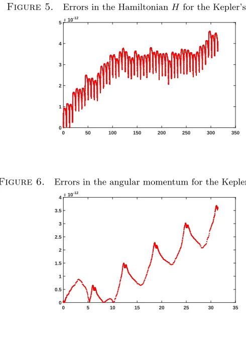
It is known that Kepler’s problem is a Hamiltonian problem and by Figures1and

2, we can see that the method does not preserve the structure for the tolerance equals to tol = 10−4. While by decreasing the tolerance to tol = 10−14, Figures 3 and 4

(10)

Figure 1. Solution of Kepler’s problem withe= 0.5,tol= 10−4_{, and} xmax= 50π.

y1

-2 -1.5 -1 -0.5 0 0.5

y2

-1 -0.5 0 0.5 1

y1

-2 -1.5 -1 -0.5 0 0.5

y2

-0.8 -0.6 -0.4 -0.2 0 0.2 0.4 0.6 0.8

Figure 3. Solution of Kepler’s problem withe = 0.5,tol= 10−14, and

xmax= 10π.

y1

-1.5 -1 -0.5 0 0.5

y2

-1 -0.5 0 0.5 1

quantities

H(y) =1 2(y

2 3+y

2 4)−(y

2 1+y

2 2)−

1/2_,

as the “Hamiltonian” of system and

(11)

y1

-2 -1.5 -1 -0.5 0 0.5

y2

-0.8 -0.6 -0.4 -0.2 0 0.2 0.4 0.6 0.8

as the “angular momentum” of system which are constant over the integration, have been plotted. This ﬁgures conﬁrm that the method is capable to conserve these quantities of the system.

Figure 5. Errors in the HamiltonianH for the Kepler’s problem.

0 50 100 150 200 250 300 350

#10-12

0 1 2 3 4 5

Figure 6. Errors in the angular momentum for the Kepler’s problem.

0 5 10 15 20 25 30 35

#10-12

(12)

5. Conclusion

A predictor-corrector method of order six based on the three-step second deriva-tive Adams-Bashforth and two-step second derivaderiva-tive Adams-Moulton was analyzed. Using Nordsieck technique, variable stepsize mode of the method was introduced and its practical implementation was discussed by preparing a starting procedure, an es-timation for the local truncation error, and changing stepsize strategy. Some system of diﬀerential equations were successfully tested.

References

[1] A. Abdi,Construction of high-order quadratically stable second-derivative general linear meth-ods for the numerical integration of stiﬀ ODEs, J. Comput. Appl. Math.,303(2016), 218–228. [2] A. Abdi, M. Bra´s, and G. Hojjati,On the construction of second derivative diagonally implicit

multistage integration methods, Appl. Numer. Math.,76(2014), 1–18.

[3] A. Abdi and G. Hojjati, An extension of general linear methods, Numer. Algor., 57 (2011), 149–167.

[4] A. Abdi and G. Hojjati,Implementation of Nordsieck second derivative methods for stiﬀ ODEs, Appl. Numer. Math.,94(2015), 241–253.

[5] A. Abdi and G. Hojjati, Maximal order for second derivative general linear methods with Runge– Kutta stability, Appl. Numer. Math.,61(2011), 1046–1058.

[6] J. C. Butcher,A modiﬁed multistep method for the numerical integration of ordinary diﬀerential equations, J. Assoc. Comput. Mach.,12(1965), 124–135.

[7] J. C. Butcher.Numerical methods for ordinary diﬀerential equations, Wiley, New York, 2008. [8] J. C. Butcher and G. Hojjati,Second derivative methods with RK stability, Numer. Algor.,40

(2005), 415–429.

[9] J. R. Cash,On the integration of stiﬀ systems of O.D.E.s using extended backward diﬀerentia-tion formulae, Numer. Math.,34(1980), 235–246.

[10] J. R. Cash,Second derivative extended backward diﬀerentiation formula for the numerical in-tegration of stiﬀ systems, SIAM J. Numer. Anal.,18(1981), 21–36.

[11] W. H. Enright, Second derivative multistep methods for stiﬀ ordinary diﬀerential equations, SIAM J. Numer. Anal.,11(1974), 321–331.

[12] A. K. Ezzeddine, G. Hojjati, and A. Abdi, Sequential second derivative general linear methods for stiﬀ systems, Bull. Iranian Math. Soc.,40(2014), 83–100.

[13] A. K. Ezzeddine, G. Hojjati, and A. Abdi,Perturbed second derivative multistep methods, J. Numer. Math.,23(2015), 235–245.

[14] E. Hairer, S. P. Nørsett, and G. Wanner, Solving ordinary diﬀerential equations I. Nonstiﬀ problems, Springer-Verlag, Berlin, 1993.

[15] S. M. Hosseini and G. Hojjati,Matrix free MEBDF method for the solution of stiﬀ systems of ODEs, Math. Comput. Model.,29(1999), 67–77.

[16] M. Hosseini Nasab, G. Hojjati, and A. Abdi, G-symplectic second derivative general linear methods for Hamiltonian problems, J. Comput. Appl. Math.,313(2017), 486–498.