Adaptive Control for Nonlinear Singular Systems
Azita Azarfar
Shahrood University of technology, Department of Electrical Engineering and Robotics, Haft Tir Sq. Shahrood, Iran
e-mail: [email protected]
Heydar Toossian Shandiz
Shahrood University of technology, Department of Electrical Engineering and Robotics, Haft Tir Sq. Shahrood, Iran
e-mail: [email protected]
Masoud Shafiee
Amirkabir University of technology, Department of Electrical Engineering Hafez Ave. Tehran, Iran
http://dx.doi.org/10.5755/j01.itc.43.2.4958
Abstract. Nonlinear singular systems present a general mathematical framework for the modeling and controlling of complicated systems, however the complex nature of this type of systems causes many difficulties in control strategy. In this paper, a model reference control approach is addressed for nonlinear affine singular systems. First, a basic control system is proposed based on the Lyapunov stability theorem so that nonlinear singular system can asymptotically track the desired linear reference model. After that, in the second design, it has been considered that systems’ parameters are unknown and two adaptive approaches are investigated. For better illustration, simulation has been done and the results show the tracking performance for both presented control systems.
Keywords: Adaptive control; affine singular systems; Model Reference control; nonlinear systems; singular control.
1. Introduction
Singular systems, which are also known as descriptor systems, differential-algebraic systems, semi-state systems, degenerate systems, constrained systems, etc. are more convenient and more precise models for realization of real systems. Singular models include both differential and algebraic equations. This class of systems has several applications in robotics, mechanical systems, electrical circuits, economic systems, chemical process systems, power systems, etc.[1-5]. Most of these models are multibody systems in which the singular model describes the dynamic behavior of the single component by differential equations and interconnection between subsystems by algebraic equations [6].
The advantage which singular systems offer in compare with ordinary differential systems is that they are easier to formulate especially in constrained systems. They have also some especial features that cannot be found in an ordinary state-space system such as they may have infinite dynamic modes which model the impulsive behavior in some systems. However, compared with ordinary state space models, they are generally more difficult to deal with.
differential equations system [6]. The systems with index zero are ordinary differential systems. Index one models can transform to ordinary state space model by one differentiation. In the systems with index one, all the constraints are explicit in model algebraic equations, but in higher index systems, there are some hidden constraints which can be observed by differentiating of the algebraic equations as many times as the system index.
Nowadays it can be claimed that most of the real systems have a singular model, and the ordinary state space model is a simplified model of the original singular one [1]. Therefore, in recent years there has been an increasing interest in singular control systems and stability analysis of such systems.
Many control approaches are rapidly extended for singular systems. Optimal control and robust methods have widely used for this class of systems [7-9]. State feedback control [10, 11], intelligent methods [12, 13] and Lyapunov based approaches [14, 15] are also extended for singular systems so far. However, few results have been reported on model reference and adaptive control. An adaptive state feedback controller for linear singular systems is investigated in [16] in which the closed-loop stability has been guaranteed by Lyapunov theory. Some model reference controller for nonlinear singular system is designed in [17, 18]. In [17] a model reference control for singular nonlinear systems with nonlinear parameterization where the nonlinearity in the parameters is convex or concave is investigated. A TS fuzzy model following control strategy is designed in [18]. As the complex nature of this type of systems causes many difficulties in control strategy, most of the control methods which have been designed so far are for linear systems, while the real systems have mostly nonlinear models. Singular nonlinear control systems are still an open research field.
Therefore, the goal of this paper is the model reference control for nonlinear affine singular systems. The objective is that the states of the nonlinear model track the states of a reference linear model. A basic controller is designed based on the Lyapunov stability theorem knowing all system parameters. After that the controller is generalized to an adaptive one. The proposed adaptive control design is divided in two sections. In the first part, it is considered that the coefficients matrix of state’s derivative, which is named E in singular systems, is known and other parameters are unknown. It is assumed that the reference system has also the same E. Then in the second part, an adaptive model reference control is designed assuming E is also unknown. Not knowing the matrix E increases the controller complexity and cost. For better illustration; both of the proposed controllers are then applied to a sample nonlinear singular system.
The paper is organized as follows. In Section 2 the problem statement is provided and the theories and assumptions used for control design are presented. In
Section 3, the basic control approach is designed based on the Lyapunov stability theorem. Adaptive control design is investigated in Section 4. Two adaptive approaches based on knowing or not knowing the matrix E are discussed there. Simulation results are presented in Section 5 and Section 6 concludes the paper.
2.Problem Statement
Consider the following nonlinear affine singular system
t
( )
t
( )
( )
u t
Ex
Ax
f x
g x
(1)where n R
x is the vector of the system’s states and
1
uR is the control input.
1
( )
nand
( )
n nR
R
g x
f x
are nonlinear function vectors. n nA R is the system matrix of linear coefficients and is a scalar. The matrix E can be singular (Rank (E) <n).
If the matrix E is invertible, then by multiplying the inverse of E, one can reach an ordinary nonlinear system which only has differential equations. But when
E
0 ( .
denotes determinant)
, the system (1) introduces a singular or descriptor system which has both differential and algebraic equations. Algebraic equations mostly are resulted from constraints which exist in the system.Now the control objective is that the nonlinear constrained system follows a desired reference linear model which is given by
t
t
t m m m mmEx A x B r (2)
where n
m
R
x
is the vector of the reference states. The matrices 1and
n n n
m
R
mR
B
A
are constant system matrices and rm is the reference model input. The matrix E in the reference model is considered to be the same as the one in the real model. It means that the degree of complexity, the number of algebraic variables and system index is similar.Choosing an appropriate reference model is a very important part of the control design. The desired reference system should be admissible. It means that the system is regular, impulse free and stable. In other words, it can be written as:
1. sEAm is not identically zero. It means
that the reference system is regular and has a unique solution.
2. degsEAm rank E
. This conditionensures that the reference system doesn’t have an impulsive response.
3. The real parts of all roots of sEAm 0
have a negative value that is equal to the stability of the reference system.
Zhang in [15] presented a stability theorem based on Lyapunov function for linear singular systems which is used here for the presented controller design.
Theorem1. The system (2) is regular, impulse free and asymptotically stable if and only if a matrix P exists which satisfies the following equations:
0
T T
m m
T T
P A A P Q E P P E
(3)where the matrix Q is positive definite [15].
Therefore it is assumed that there is a matrix P with which the reference model (
E, A
m ) satisfies (5)in Theorem 1.
To define a linear system as a reference model for the nonlinear one, there are some more conditions that should be satisfied. If the nonlinear singular system (1) is rewritten as
t
A
1( )
( )
u t
Ex
x x g x
(4)then there are some matching (or perfect model following) conditions which guarantee that the equality xxm can be obtained. These conditions were established by several works (for instance, [19-21]) for ordinary differential systems. Because the matrix E in the nonlinear plant and in the reference model is the same, these conditions can also be generalized for singular systems according to the proof in [20, 21]. The matching condition can be expressed as rankrequirements:
1
(R( ) denotes ( ))
( ) ( ),
( ) ( )
m
m a Rang a
R R
R R
g A A
g B (5.a)
or
† †
1
(
I gg B
)
m
0 ;
(
I gg
)(
A
m
A
)
0
(5.b) where † 1( T ) T
g g g g is the pseudo-inverse of g. It is
obvious that the both conditions are equivalent. It is assumed that the proposed reference model satisfies the conditions in (5).
After choosing an appropriate linear reference model, by defining the tracking error vector as
m
e x x
(6)and by subtracting (2) from (1), the closed loop dynamics would be as
t
m
( )
m
( )
u
m mr
Ee
A e Ax
f x
A x g x
B
.(7)For simplifying the equations, the following definition is introduced:
ˆ( )
( )
mf x
Ax
f x
A x
. (8)So, the error dynamic of the closed loop system would be as follows:
t m ˆ( ) ( )u m mrEe A e f x g x B . (9)
Now the control objective is to find 𝑢 such that the tracking error tends to zero as fast as possible.
3. Basic Control Design
In the first step, it is assumed that all parameters of the system are known, and tracking the states in reference model is the objective of the control design. In mathematical view, the error term in (9) tends to zero. The control law is directly extracted from Lyapunov function. The convergence rate depends on the reference model, as the reference model poles define how fast the tracking error tends to zero.
In order to find a control law, which would fulfill our goal and guarantee the stability, the following Lyapunov function is proposed:
T T
Ve E Pe (10)
where P satisfies (3).
Differentiating V results in
T T T T
Ve E Pee P Ee (11)
Using (9), one can get ˆ
( ) 2 [ ( ) ( ) ].
T T T T T
m m m m
Ve A PP A e e P f x g x uB r (12) Now it is clear that if u is chosen in the way that the equation
ˆ
( )x u ( )x m mr
g f B (13)
is satisfied, then the derivative of V would be as follows:
T
V e Qe (14)
Based on the Lyapunov stability theorem, the tracking error tends to zero and the nonlinear system follows the desired reference model. Equation (13) is a non-square matrix equation that can be solved in many ways. If g(x) is a vector, one solution would be as follows:
† ˆ
( ( ) m m)
ug f x B r . (15) When u is eliminated from (15) and (13), the zero error condition can be express as:
† ˆ
Using (8) and (4), the condition in (16) can be rewritten as
† 1
(
I gg
)( (
A
A x B
m)
m mr
)
0
. (17) It can be easily proved, the equation (17) can be obtained from matching conditions (5). In other words, the matching conditions (5) guarantee that (17) will be hold for all values of x andrm. So, as a result, it can be obtained that the proposed control law (15) satisfies (13).So, by choosing the control law (15), the error dynamic would be as
m
Ee A e. (18)
Therefore the poles of the system (E A, m), which are the roots of sEAm 0 , define the error decreasing rate.
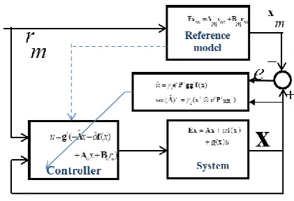
As a conclusion, if all the system parameters are known and the control law is chosen as in (15), then all the states of nonlinear singular system (1) track the states of the linear reference model (2). The control system is summarized in Figure 1. In the second step, as discussed in the following section, some system parameters are considered to be unknown and two adaptive approaches are designed based on known and unknown matrix E.
4. Adaptive Control Design
In the first approach, it is assumed that the matrix A and the scalar are unknown but fixed. It means that the nonlinear dynamics structures are known but system parameters are unknown. For this situation, the following control law is proposed:
(19) where 𝐀̂ and 𝛼̂ stand for estimation of A and , respectively. Multiplying g in both sides of (19) and adding and subtracting some terms, results in
(20) Considering matching condition (5), the equation (20) can be rewritten as
. (21)
Now by substituting (21) in the error dynamic system (7), the closed loop system would be as
. (22) From (22) it is clear that, if 𝐀̂ and 𝛼̂ is equal to 𝐀
and 𝛼respectively, then the error asymptotically tends to zero.
Figure 1. Basic control system structure
Now, to guarantee the stability and to decrease the parametric error, the following Lyapunov function is the candidate:
2
1 2
1 1 ˆ ˆ
ˆ
( ) ( )T ( )
T T
V vec vec
e E Pe AA AA (23) where P satisfies (3) and vec(A) denotes vectorization of A, which is obtained by stacking the columns of the matrix A on top of one another. It is a linear transform which converts the matrix into a column vector. Using vec(A) and Kronecker product makes the computations more simple.
Differentiating the Lyapunov function with respect to t results in
1
2
2
ˆ ˆ
( )
2 ˆ ˆ
( ) ( )
T T T T
T
V
vec vec
e P Ee e E Pe
A A A
. (24)
Considering the system dynamic (22), the Lyapunov derivative can be rewritten as
.(25)
It can be written as:
(26) as the term 𝐞 𝐏 𝐠𝐠 (𝐀 − 𝐀̂)𝐱 is scalar, this term can be written as
(27) and due to the Kronecker product properties, it is equal to
† ˆ ˆ
( ( ) m m m)
ug Axf x A xB r
† ˆ ˆ
( ( ) m m m ( ) ( ) ( ))
u r
g gg Ax f x A x B A A x f x
†
(
( )
)
ˆ
ˆ
((
)
(
) ( ))
m m m
u
r
g
Ax
f x
A x
B
gg
A
A x
f x
†
ˆ
ˆ
((
)
(
) ( ))
m
Ee
A e gg
A A x
f x
†
1 2
ˆ ˆ
( ) 2 (( ) ( ) ( ))
2 2 ˆ ˆ
ˆ ˆ
( ) ( ) ( )
T T T T T
m m
T V
vec vec
e A P P A e e P gg A A x f x
A A A
† 1 1
†
2 2
ˆ ˆ
( )[ ( )]
2
ˆ ˆ ˆ
2 ( ) ( ) ( )
T T T
T T T
V
vec vec
e Qe e P gg f x
e P gg A A x A A A
† ˆ † ˆ
( ) ( ( ) )
T T T T
vec
. (28) So, the derivative of Lyapunov functions (26) would be as
.
(29)
Now by defining the parameters updating law as
(30)
the derivative of Lyapunov function can be written as
. (31)
By the proposed updating mechanism, the stability would thus be guaranteed and the tracking error tends to zero. The adaptive model reference control structure is summarized in Figure 2.
In the second approach, it is considered that matrix E of the system is also unknown and it is different from 𝐸 in the reference model. This assumption makes the control system more complicated.
4.1. Unknown Matrix E
In this part, it is assumed that the parameters E,A and in the nonlinear model (1) are unknown and the objective is tracking a linear singular model with different E like
(32)
where 𝐄 , 𝐀 should satisfy (3). Unknown E increases the complexity of the control design and cost. The matrix E is not just a coefficient, it demonstrates the system index and it is in charge of complexity of the system. In this section, the system may be forced to track a reference model with a different index or even a non-singular system ( ). However to obtain such an advantage, the design difficulty and the cost should be tolerated.
First, the matching conditions (5) must be reviewed. Some conditions on 𝐄 will be added because 𝐄 in the reference model is different from E in the real system. According to the proof in [21], it can easily be resulted that the rang of g must contain the rang of (𝐄 − 𝐄), as
(33.a) Or
(34.b)
Figure 2. Adaptive model reference control system
while the exact value of the system parameters is unknown, but it is assumed that the system matrices satisfy the matching conditions (5) and (33). It is not an unpractical assumption because the matching conditions are originally rank requirements, and it is natural to know about the ranks and degree of the system which is under control. For example, to control a DC motor, the dynamics structures and ranks are known, however the value of parameters, such as armature resistance and coefficients, may not be available. To fulfill the goals, the system (32) is subtracted from (1). Then using (6) results in
(34)
which is the dynamics of tracking error. Now the objective is that the tracking error tends to zero. A control law is proposed as
(35) where 𝐄̂, 𝐀̂ and 𝛼̂ are estimations of E, A and , respectively. As it has been shown, a state derivative feedback term is added to the controller. Using state derivative feedback is very useful and typical in singular systems because it can directly affect the index and regularity of closed-loop systems. However in ordinary differential systems, performance of the state derivative feedback control is not different from usual state feedback. So, it is not usually applied there. Now according to matching conditions (5), (33) and multiplying g in both sides of (19) results in
.(36)
By substituting (20) in system dynamic (34), the closed-loop error dynamic system can be given by
(37) Now, to stabilize the system and decrease the parameter errors, the following Lyapunov function is defined:
† ˆ † ˆ
( T T ( ) ) ( T T T ) ( )
vece P gg AA x x e P gg vecAA
† 1 1
† 2
2
2 ˆ ˆ
( )[ ( )]
2 ˆ ˆ
[ ( ) ( )] ( )
T T T
T T T T
V
vec vec
e Qe e P gg f x
A x e P gg A A
† 1
† 2
ˆ ( )
ˆ
( ) ( )
T T
T T T T
vec
e P gg f x
A x e P gg
T
V
e Qe
t
t
tm m m
m m m
E x A x B r
0
E
( )
(
m)
R
g
R
E
E
†
(
I gg
)(
E
m
E
)
0
(
( )
)
( )
(
)
m m m
m m m
t
u
r
E e
A e
Ax
f x
A x
g x
B
E E x
† ˆ ˆ ˆ
( ( ) m m m ( m) )
ug Axf x A xB r EE x
†
( ( ) ( ) )
ˆ ˆ ˆ
(( ) ( ) ( ) ( ) )
m m m m
u r
g Ax f x A x B E E x
gg A A x f x E E x
† ˆ ˆ ˆ
(( ) ( ) ( ) ( ) )
m m
(38)
The Lyapunov derivative can be written as
.(39)
Similar to (25) – (29), (39) can be rewritten as
.(40)
So, by choosing the adaption law as
(41)
the Lyapunov derivative function will be negative as
(42) and the tracking error tends asymptotically to zero. Adding state derivative feedback to control law makes the controller more complicated. The vector cannot directly be calculated from equations in singular systems, as some state variables appear just algebraically. By differentiating, the vector can be obtained. As we know, differentiating may add some extra noise to the system and increase the computational efforts; however, due to better control performance and the advantages of tracking a reference model with different index, it is acceptable. The structure of adaptive model reference control with unknown E is summarized in Figure 3.
For better illustration, simulation has been done as reported in the following section. It is clear that by using the simple control (15) the reference model’s poles are responsible for convergence rate. Since the reference model 1 has one pole in s= -4, good tracking rate is obtained, which confirms the mentioned claim. In simulation B, following system (27) the reference model 2 is the objective of the adaptive control.
5. Simulation Results
In order to illuminate the two discussed approaches more clearly two simulations have been
Figure 3. Adaptive model reference control system with unknown E
performed. In the first simulation, the controller is applied to a typical numerical system introduced by (43) and in the second one, we use the proposed method for reference model tracking of a nonlinear mass-spring-damper system modeled by singular systems.
5.1. Simulation on numerical system
Consider the nonlinear affine singular system (1) with the following matrices:
.(43)
The control objective is that the system (27) follows two different linear reference systems. The reference models are defined as follows.
Reference model 1 is
(44)
which is singular and introduced for the first approach where E is known and similar to 𝐄 . The reference model 2 is defined as
(45) where 𝑟 = sin(0.5𝜋𝑡).
The reference model 2 is not singular (|𝐸| ≠ 0). It is defined for the second proposed approach. Both of the models satisfy matching conditions. Two simulation scenarios have been considered which are investigated in the following subsections.
5.1.1. Simulation A
In this simulation scenario, the objective is that the nonlinear system (43) follows the reference model 1 2
1 2
3
1 ˆ 1 ˆ ˆ
( ) ( ) ( )
1 ˆ ˆ
( ) ( )
T
m
T
T T
V vec vec
vec vec
e E Pe A A A A
E E E E
†
1
2 3
ˆ
( ) 2 (( )
2 ˆ
ˆ ˆ ˆ
( ) ( ) ( ) ) ( )
2 ˆ ˆ 2 ˆ ˆ
( ) ( ) ( ) ( )
T T T T T
m m
T T
V
vec vec vec vec
e A P P A e e P gg A A x
f x E E x
A A A E E E
† 1 1 † 2 2 † 3 3 2 ˆ ˆ ( )[ ( )]
2 ˆ ˆ
[ ( ) ( )] ( )
2 ˆ ˆ
[ ( ) ( )] ( )
T T T
T T T T
T T T T
V vec vec vec vec
e Qe e P gg f x
A x e P gg A A
E x e P gg E E
† 1 † 2 † 3 ˆ ( ) ˆ ( ) ( ) ˆ ( ) ( ) T T
T T T T
T T T T
vec vec
e P gg f x
A x e P gg
E x e P gg
T
V
e Qe
x
x
1
1
0
1 0 3 2 0
, A , 1 , ,
cos
0 0 0 1 x
x e
E f g
1 1
2 2
1 0 3 2 0
0 0 1 2 1
m m m m m x x r x x
1 1 2 21 0 3 2 0
1 1 1 2 1
Figure 4. State of x1, following the reference model 1 using controller (18). The matrix E is similar
in real and reference systems
Figure 6. Tracking error in simulation A
Figure 5. state of x2, following the reference model 1 using controller (18). The matrix E is similar in real
and reference systems
Figure 7. Control input in simulation A
(44) using the adaptive control (18) and the adaption mechanism (26). The matrix A and are considered to be unknown during the simulation. Their initial values are set to zero.
Simulation results emphasize that good tracking performance has been obtained. Figures 4-7 display the system performance. Tracking the reference model by system states is shown in Figures 4 and 5. The states of x1 and x2 completely track the reference states of xm1 and xm2. Figure 6 shows the tracking error tending to zero; and in Figure 7, the control input is displayed which is smooth and bounded.
Now in simulation B, the objective is that the system (43) follows the reference model 2 (45).
5.1.2. Simulation B
This simulation has been done to discuss the case where the matrix E is also unknown. In this part, the objective is that the nonlinear singular system follows the non-singular reference model 2 using the control law (35) and the adaption rules (41). The matrices E,
A and 𝛼 are considered to be unknown. The derivative array is needed and should be calculated.
The controller is applied to the system and the results are shown in Figures 8-11. Tracking performance is displayed in Figures 8 and 9. It’s clear that the system’s states tend to the reference model. The tracking error is shown in Figure 10. It tends to zero. As it is shown, when the matrix E is also unknown, the convergence takes more time because there are more parameters which should be adjusted. The control input is shown in Figure 11. The results show that the proposed controller has completely coped with tracking a system with a different index even with an unknown E.
From all simulation results on sample system, it is clear that both discussed control systems are well-behaved and have desirable performance. For better illustration of control performance, another simulation is also done on a mechanical system. Simulating the proposed control on a nonlinear mass-spring-damper system is investigated in the following section.
0 5 10 15 20 25 30 -0.3
-0.2 -0.1 0 0.1 0.2 0.3 0.4
Time(s)
x1
x1 xm1
0 5 10 15 20 25 30 -0.2
-0.1 0 0.1 0.2 0.3 0.4 0.5
Time(s)
T
ra
c
ki
n
g
e
rr
o
r
e1 e2
0 5 10 15 20 25 30 -0.6
-0.4 -0.2 0 0.2 0.4 0.6
Time(s)
x2
x2 xm2
0 5 10 15 20 25 30
-1.8 -1.6 -1.4 -1.2 -1 -0.8 -0.6 -0.4 -0.2
Time(s)
C
o
n
tr
o
l
in
p
u
t
Figure 8. Following the non-singular reference model 2 using controller (34), state of x1
Figure 10. Tracking error in simulation B, the error tends
to zero asymptotically
Figure 9. Following the non-singular reference model 2 using controller (34), state of x2
Figure 11. Control input in simulation B, it is smooth and bounded
5.2. Simulation on nonlinear mass-spring-damper system
Consider the mass-spring-damper system with spring hardening and position dependent mass described by:
2 3
0 1
(1
)
m
q q bq k q k q
u
(46)where q is the displacement of position dependent mass m and 𝑘 , 𝑘 are nonlinear spring constants. The parameter b is damping coeficient of the damper. By choosing the state variables as
1 2 3
[
x x x
]
T[
q q q
]
T
x
(47)the system dynamics can be rewritten in singular form similar to (1) using the following matrices:
0
3 2
1 1 1 3
1
0
0
0
1
0
0 1
0
0
0
1
0
0
0
0
0
( )
0
0
1
1
k
b
m
k x
mx x
E
A
f x
g
. (48) It is possible to model this mechanical system using just two differential equations in ordinary state space, but by using the singular model of the mass-spring-damper system we can reach more precise model which can also describe the behavior of accelration of the mass.
Moreover, we can also control the mass accelaration respect to algebraic constraint appeared in the third equation in (48).
Similar to the previouse simulation, two poroposed control strategies are applied to system (48). Two different reference models are also defined as:
0 5 10 15 20 25 30 -0.4
-0.2 0 0.2 0.4 0.6
Time(s)
x1
x1 xm1
0 5 10 15 20 25 30 -0.8
-0.6 -0.4 -0.2 0 0.2 0.4
Time(s)
T
ra
c
ki
n
g
e
rr
o
r
e1 e2
0 5 10 15 20 25 30
-1.5 -1 -0.5 0 0.5 1
Time(s)
x2
xm2 x2
0 5 10 15 20 25 30
-2.5 -2 -1.5 -1 -0.5 0 0.5
Time(s)
C
o
n
tr
o
l
in
p
u
Reference model 3:
1 1
2 2
3 3
1 0 0 0 1 0 0
0 1 0 0 0 1 0
0 0 0 6 5 1 2
m m
m m m
m m
x x
x x r
x x
(49)
which is singular and introduced for the first approach where E is known and is similar to 𝐄 . The reference model 4 is defined as
1 1
2 2
3 3
1 0 0 0 1 0 0
0 1 0 0 0 1 0
0 0 1 6 11 6 2
m m
m m m
m m
x x
x x r
x x
. (50)
The reference model 4 is not singular and is introduced for the second approach.
The selected reference input 𝑟 is shown in Fig. 12. Two different simulations for tracking the two proposed reference models are investigated in the following subsections. The model parameters are set to 𝑚 = 1, 𝑘 = 1, 𝑘 = 1 and 𝑏 = 1.
5.2.1. Simulation C
In this sub-section, the objective of the control is tracking the states of the linear reference model (49) using the adaptive control (18) and the adaption
mechanism (26). The matrix A and 𝛼 are considered to be unknown during the simulation. Control system simulation results are shown in Figures 13-15.
The states’ responses tracking desired states are displayed in Figure 13. As Figure 14 shows the tracking error is acceptable and tends to zero. The control input is displayed in Figure 15. The simulation results emphasize the effectiveness of the proposed controller.
Now in the following subsection, simulation of tracking the reference model 4 is investigated.
5.2.2. Simulation D
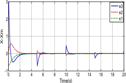
In this part the objective of the control is following the non-singular reference model 4 using the control law (35) and the adaption rules (41). The matrices E, A and 𝛼 are considered to be unknown. The controller is applied to the system and the results are displayed in Figures 16-18. Figure 16 shows the states’ responses. Figure 17 shows the tracking error and the control input is displayed in Figure 18. As the results show, the controller is successfully tracking a non-singular model.
All simulation results emphasize the acceptable performance of both proposed control approaches.
Figure 12. the reference input in simulation C and D
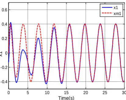
Figure 13. The states’ response tracking reference model (49) in simulation C
Figure 14. Tracking error in simulation C
Figure 15. Control input in simulation C
0 2 4 6 8 10 12 14 16 18 20 0
0.5 1 1.5 2
Time(s)
r(
m
)
Reference Signal
0 2 4 6 8 10 12 14 16 18 20 0
0.5 1
x1
0 2 4 6 8 10 12 14 16 18 20 -1
0 1
x2
0 2 4 6 8 10 12 14 16 18 20 -5
0 5
Time(s)
x3
xm2 x2 xm1 x1
xm3 x3
0 2 4 6 8 10 12 14 16 18 20
-1 0 1 2 3
Time(s)
X
-X
m
e3 e2 e1
0 2 4 6 8 10 12 14 16 18 20
-4 -3 -2 -1 0 1 2 3 4
Time
Figure 16. The states’ response tracking reference model
(50) in simulation D
Figure 17. Tracking error in simulation D
Figure 18. Control input in simulation D
6. Conclusion
In this paper, the model reference control for nonlinear affine singular systems has been investigated. A basic non-adaptive control structure has been proposed and was generalized to two different adaptive control approaches. The stability of all controllers was proved using Lyapunov stability theorem. In the first adaptive control system, it is assumed that some system parameters are unknown but the matrix E which is in charge of the complexity and system index is known. The controller is very simple, practical and shows good performance. In the second adaptive control approach, the matrix E is also considered to be unknown. The control cost and complexity increase, but it has a good performance even in tracking a non-singular system. Simulation results showed a desirable tracking performance for the both proposed control systems.
References
[1] L. Dai. Singular control systems. Springer-Verlag, New York, Inc., 1989.
[2] F. L. Lewis. A survey of linear singular systems.
Circuits, Systems and Signal Processing, 1986, Vol. 5, No. 1, 3-36.
[3] D. G. Luenberger, A. Arbel. Singular dynamic Leontief systems. Econometrica: Journal of the Econometric Society, 1977, Vol. 45, No. 32, 991-995. [4] L.-S. You, B.-S. Chen. Tracking control designs for
both holonomic and non-holonomic constrained mechanical systems: a unified viewpoint. International Journal of Control, 1993, Vol. 58, No. 3, 587-612. [5] R. Gani, I. T. Cameron. Modelling for dynamic
simulation of chemical processes: the index problem.
Chemical Engineering Science, 1992, Vol. 47, No. 5, 1311-1315.
[6] P. Müller. Descriptor systems: pros and cons of system modelling by differential-algebraic equations.
Mathematics and Computers in Simulation, 2000, Vol. 53, No. 4, pp. 273-279.
[7] M. Shafiee, P. Karimaghai, Optimal control for singular systems (Rectangular case). In: Proc. of ICEE'97, 1997, pp. 152-160.
[8] D. Bender, A. Laub. The linear-quadratic optimal regulator for descriptor systems. Automatic Control, IEEE Transactions on, 1987, Vol. 32, 672-688. [9] A. V. A. Kumar, P. Balasubramaniam. Optimal
control for linear singular system using genetic programming. Applied Mathematics and Computation,
2007, Vol. 192, 78-89.
[10] E. Boukas. Static output feedback control for linear descriptor systems: LMI approach. In: Mechatronics and Automation, 2005 IEEE International Conference, 2005, pp. 1230-1234.
[11] M. Dodig, M. Stošić. Singular systems, state feedback problem, Linear Algebra and its Applications, 2009, Vol. 431, No. 18, 1267-1292.
[12] Y. Wang, Z.-Q. Sun, F.-C. Sun. Robust fuzzy control of a class of nonlinear descriptor systems with time-varying delay. International Journal of Control, Automation and Systems, 2004, Vol. 2, No. 1, 76-82. [13] S.-L. Tung, Y.-T. Juang, W.-H. Lee, H.-C. Chiu. An
improved particle swarm optimization for exponential stabilization of a singular linear time-varying system.
Expert Systems with Applications, 2011, Vol. 38, 13425-13431.
[14] K. Takaba, N. Morihira, T. Katayama. A genera-lized Lyapunov theorem for descriptor system. Systems & Control Letters, 1995, Vol. 24, No. 1, 49-51. [15] Q. Zhang, J. Lam, L. Zhang. Generalized Lyapunov
equation for analyzing the stability of descriptor systems. In: Proceedings of the 14th World Congress of IFAC, 1999, pp. 19-24.
[16] A. Azarfar, H. T. Shandiz, M. Shafiee. Adaptive feedback control for linear singular systems. Turkish 0 2 4 6 8 10 12 14 16 18 20
0 0.5 1
x1
0 2 4 6 8 10 12 14 16 18 20 -0.5
0 0.5
x2
0 2 4 6 8 10 12 14 16 18 20 -1
0 1
Time(s)
x3
xm x
0 2 4 6 8 10 12 14 16 18 20 -1
-0.5 0 0.5 1
Time(s)
X
-X
m
e1 e2 e3
0 2 4 6 8 10 12 14 16 18 20
-0.5 0 0.5 1 1.5 2
Time(s)
Journal of Electrical Engineering & Computer Sciences, 2014, Vol. 22, 132-142.
[17] Q. Fang, F. Cao. Adaptive control of singular nonlinear systems with convex/concave parametrization. In: Control Automation Robotics & Vision (ICARCV), 2010 11th International Conference on, 2010, pp. 1680-1683.
[18] D. Wang, S. Wu, S. Okubo, T. Akiyama. TS fuzzy model following control system for descriptor system. In: Computer-Aided Industrial Design & Conceptual
Design, 2009, AID & CD 2009, EEE 10th International Conference on, 2009, pp. 2275-2279. [19] A. Balestrino, G. De Maria, A. Zinober. Nonlinear
adaptive model-following control. Automatica, 1984, Vol. 20, No. 5, 559-568.
[20] Y. T. Chan. Perfect model following with real model. In: Proceedings Joint Autom. Control Conference, 1974, pp. 287-293.
[21] H. Erzberger. Analysis and design of model following control systems by state space techniques. In: Proc. of JACC, pp.572-581, 1968.