BioMedCentral
Page 1 of 15 (page number not for citation purposes)
International Journal of Health
Geographics
Open Access
Research
Developing a spatial-statistical model and map of historical malaria
prevalence in Botswana using a staged variable selection procedure
Marlies H Craig*
1,2, Brian L Sharp
1, Musawenkosi LH Mabaso
1,2and
Immo Kleinschmidt
1,3Address: 1Malaria Research Programme, Medical Research Council, 491 Ridge Road, Overport, Durban, 4091, South Africa, 2Swiss Tropical Institute, 57 Socinstrasse, Basel, BS 4002, Switzerland and 3London School of Hygiene and Tropical Medicine, Keppel Street, London WC1E 7HT, UK
Email: Marlies H Craig* - [email protected]; Musawenkosi LH Mabaso - [email protected]; Immo Kleinschmidt - [email protected]
* Corresponding author
Abstract
Background: Several malaria risk maps have been developed in recent years, many from the prevalence of infection data collated by the MARA (Mapping Malaria Risk in Africa) project, and using various environmental data sets as predictors. Variable selection is a major obstacle due to analytical problems caused by over-fitting, confounding and non-independence in the data. Testing and comparing every combination of explanatory variables in a Bayesian spatial framework remains unfeasible for most researchers. The aim of this study was to develop a malaria risk map using a systematic and practicable variable selection process for spatial analysis and mapping of historical malaria risk in Botswana.
Results: Of 50 potential explanatory variables from eight environmental data themes, 42 were significantly associated with malaria prevalence in univariate logistic regression and were ranked by the Akaike Information Criterion. Those correlated with higher-ranking relatives of the same environmental theme, were temporarily excluded. The remaining 14 candidates were ranked by selection frequency after running automated step-wise selection procedures on 1000 bootstrap samples drawn from the data. A non-spatial multiple-variable model was developed through step-wise inclusion in order of selection frequency. Previously excluded variables were then re-evaluated for inclusion, using further step-wise bootstrap procedures, resulting in the exclusion of another variable. Finally a Bayesian geo-statistical model using Markov Chain Monte Carlo simulation was fitted to the data, resulting in a final model of three predictor variables, namely summer rainfall, mean annual temperature and altitude. Each was independently and significantly associated with malaria prevalence after allowing for spatial correlation. This model was used to predict malaria prevalence at unobserved locations, producing a smooth risk map for the whole country.
Conclusion: We have produced a highly plausible and parsimonious model of historical malaria risk for Botswana from point-referenced data from a 1961/2 prevalence survey of malaria infection in 1–14 year old children. After starting with a list of 50 potential variables we ended with three highly plausible predictors, by applying a systematic and repeatable staged variable selection procedure that included a spatial analysis, which has application for other environmentally determined infectious diseases. All this was accomplished using general-purpose statistical software.
Published: 24 September 2007
International Journal of Health Geographics 2007, 6:44 doi:10.1186/1476-072X-6-44
Received: 25 April 2007 Accepted: 24 September 2007
This article is available from: http://www.ij-healthgeographics.com/content/6/1/44 © 2007 Craig et al; licensee BioMed Central Ltd.
Background
Recent years have seen widespread application of geo-graphic information systems and spatial statistical meth-ods in modelling and mapping the distribution of vector borne diseases, including malaria. In sub-Saharan Africa the Mapping Malaria Risk in Africa (MARA) project has been working towards a malaria risk atlas for rational and targeted control of the disease [1]. To this end historical and current survey data have been collated of the preva-lence of infection with human Plasmodium parasites.
A number of malaria risk maps, at country and regional level, have been produced by analysing geo-referenced prevalence data against environmental data to predict prevalence at localities where it was not recorded [2-6]. Different analytical approaches of varying sophistication have been explored. Multiple variable logistic regression analysis, commonly used to assess the odds of infection against potential risk factors, has been employed, and the spatial dependence in the response data has been mod-elled most successfully using Bayesian spatial modelling. One outstanding issue, which can greatly affect the predic-tions, remains the variable selection procedure, particu-larly when there are a large number of potential risk factors.
In regression analysis and predictive/prognostic statistics, model validity is an important aspect [7], both the inter-nal validity, or accuracy, i.e. the model explains the observed data well, and external validity, or generalizabil-ity, i.e. the model predicts new data well. In this context we furthermore aim for parsimony (model contains a few strong predictors that are easily interpretable) and plausi-bility, both of the co-variates (association with the disease are etiologically explainable) and of the predictions (believable in view of what is generally known). Taking account of the spatial correlation structure in the data is important for "geographic transportability", i.e. when pre-dicting malaria prevalence to unobserved locations [8].
Selecting a few predictors for spatial modelling from among a large number of potential candidates is a major challenge and can easily become arbitrary. Ideally every possible combination of variables would be tested and compared in a Bayesian spatial framework. However, this would be extremely computing-intensive and unfeasible, if not impossible, for most users. The most practical route is to reduce the list of potential explanatory variables using non-spatial selection methods, before moving to a spatial context.
Neither manual nor automated stepwise selection proce-dures are advised, because of frequent over-fitting, and because of the resulting "phantom degrees of freedom" [9] pg 416: testing and rejecting many variables increases
the probability of finding a significant predictor by chance, but since this sifting remains undeclared, stand-ard errors in the final model are underestimated. Babyak [9], citing Harrell [10] and others, recommend shorter lists of candidate predictor variables, which are not strongly correlated, as well as bootstrapping, as a form of simulation. Austin and Tu [11], working on heart attack data, developed their model by running repeated step-wise selection procedures on bootstrap samples of their data, to identify the most consistent predictors.
The aim of this study was to develop a map of historical malaria risk for Botswana by analysing malaria prevalence data against a number of environmental variables from different data themes, using a systematic and repeatable staged process of variable elimination, including the step-wise bootstrap method described by Austin and Tu [11]. The resulting small subset of variables, each independ-ently associated with the response, but possibly spurious because the condition of spatial independence was not satisfied, was tested in a Bayesian geo-statistical model. We used the spatial model derived from the observed locations, to predict prevalence of malaria infection in children 1–14 years old at unobserved map locations across the whole country.
Methods
Study areaBotswana is semi-arid to arid with few permanent water bodies. The country is flat, mostly between 900 and 1200 m altitude. The rainy season is from November to March. Vegetation ranges from desert scrub-land in the South-West, where annual rainfall is <300 mm, through grass-land, to wooded savannah in the North, which receives >500 mm rain annually. Mean annual temperatures are between 18 and 23°C. Botswana today has a total popu-lation of about 1.6 million; popupopu-lation density over two thirds of the country being <1 per square km [12]. The population according to the 1971 census was 630379 with an approximate 3.1% annual increase [13] which if extrapolated back in time translates to around 470000 in 1961/62. In 1975 80% of the population lived in the east-ern part of the country,
International Journal of Health Geographics 2007, 6:44 http://www.ij-healthgeographics.com/content/6/1/44
Page 3 of 15 (page number not for citation purposes) between 1961/62 and 1974, and further thereafter [14].
By 1960 no prevalence above 70% was measured, suggest-ing meso-to hypo-endemic conditions. Further South, transmission is hypo-endemic and epidemic, and over large areas entirely absent. Incidence, like the climate, is strongly seasonal, peaking around March/April [16]. The gradient in malaria broadly follows the environmental gradients described before.
Malaria data
Archived malaria prevalence data were collated within the MARA project, as described by Omumbo et al [17]. In Bot-swana geographical coordinates could be obtained for 613 out of a total of 1063 age-specific prevalence surveys. Of these, 20 did not report sample sizes and were excluded. Here we used only the 1961/62 national survey (figure 1) to develop a historical malaria risk map. For the 1–14 year age group, 122 prevalence results were availa-ble, for 118 unique locations across the country,
progres-sively from August 1961 to May 1962. Surveys in different regions were carried out during different months (figure 2). The total number examined was 17149; the mean sam-ple size was 141 per survey (range 2–831). The design effect was calculated in Stata [18].
Environmental data
Forty-nine variables representing different summaries and transformations of the eight environmental data themes (see table 1), were included in the study: elevation [19], surface water [20], land cover [21], long-term monthly mean rainfall, temperature [22], vapour pressure [23], and normalized difference vegetation index (NDVI) at 8 km [24] and 1 km [25] resolution.
Themes with monthly values (rainfall, temperature, NDVI and vapor pressure) were plotted against logit-trans-formed malaria prevalence, logit(p). Based on observed temporal patterns in the scatter plots, months were
aggre-Malaria prevalence data
Figure 1
gated for "summer" (December to March) and "winter" (April to October). Different annual summary indices were also calculated for each theme. Calculations of some of the variables are shown in the appendix.
Distance from water bodies was calculated by projecting maps of perennial and non-perennial water bodies onto a 200 × 200 m grid and calculating for each grid cell the euc-lidian distance to the nearest water body. Values were transformed by adding a value of 100 m to each pixel and deriving the natural logarithm.
For land cover, the thirteen United States Geological Sur-vey land cover classes occurring in Botswana were re-grouped into two categories, broadly corresponding to drier and moister land cover types. Most data points were found in "grassland" and "savannah" with only isolated surveys in the other land cover types. Prevalence was gen-erally higher in "savannah" than in "grassland" areas. Other obviously drier and lower risk land cover types ("barren or sparsely vegetated", "shrub land", "urban or built-up") were therefore included with "grassland" in a "low risk" category, while other clearly moister classes ("herbaceous wetland", "water bodies", "evergreen broad-leaf forest") were included with the higher-risk "savan-nah" category. Other minor land cover types were included in the category alongside which they mostly
commonly occurred ("grassland/crop land mosaic" was mainly found scattered among "grassland"; "dryland crop land and pasture" and "mixed" among "savannah").
Values were extracted from the data grids for each geo-graphical location where a malaria survey result was avail-able.
Variable selection and model development
We carried out a staged approach during model formula-tion. A flow chart of the variable selection procedure is shown in figure 3.
Stage 1
The malaria prevalence database was split randomly into derivation (n = 81) and validation (n = 41) sub-sets. To identify the best univariate predictors, univariate logistic regression analysis against the derivation data was carried out on all 50 potential predictors. We allowed for cluster-ing by survey location uscluster-ing the Hubert-White sandwich estimator in Stata [18].
Stage 2
To reduce confounding arising from correlated variables, and also to reduce the variables to data ratio, we ranked the variables significant in univariate analysis by the Akaike Information Criterion [26] (AIC), and excluded those that were strongly correlated (Spearman's r > 0.85) with a higher-ranking variable belonging to the same environmental theme. Scatter plots against logit(p) were prepared of the remaining variables (figure 4).
Stage 3
Following the approach of Austin and Tu [11], we drew 1000 bootstrap samples from the derivation data, and ran automated backward exclusion procedures on each sam-ple. Since it was not possible in Stata to allow for cluster-ing within the stepwise procedure, which resulted in the explanatory power of variables being over-estimated, we used stringent entry and removal thresholds (p = 0.02 and 0.05 respectively). We recorded the co-efficients and the number of times each candidate variable was selected in the 1000 models.
Stage 4
A non-spatial multiple-variable model was derived in a manual step-wise fashion, starting with the most fre-quently selected variable, and adding further variables in order of selection frequency, as long as all entered varia-bles remained significant at the 5% probability level. If a previously entered variable became non-significant with the addition of another, we retained the one more fre-quently selected in Stage 3 in favour of the other.
Month of survey during the 1961/62 national malaria survey
Figure 2
International Journal of Health Geographics
2
007
,
6
:44
http://www.ij-h
ealthg
eog
ra
phi
cs.com/content/6/1/4
4
Pa
ge 5 of
1
5
(page number not for citation purposes)
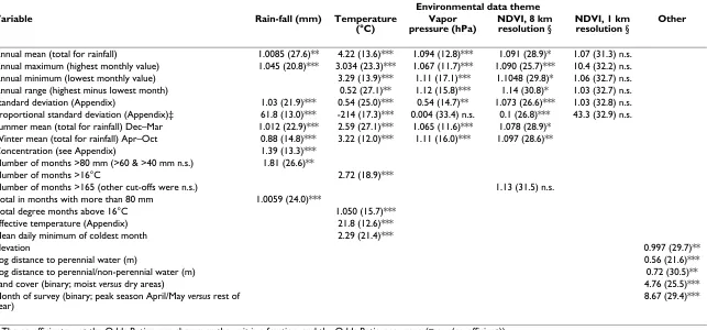
Table 1: Results of uni-variate analysis from Stage 1. Odds Ratios (AIC in parentheses) from univariate logistic regression analysis of 50 different environmental variables from 7 themes, against malaria prevalence. P-values were non-significant (n.s.), <0.05(*), <0.01(**) or <0.0005 (***), n = 122. The equation was logit(prevalence) = coefficient × co-variate + constant. NDVI = normalized difference vegetation index.
Environmental data theme
Variable Rain-fall (mm) Temperature
(°C)
Vapor pressure (hPa)
NDVI, 8 km resolution §
NDVI, 1 km resolution §
Other
Annual mean (total for rainfall) 1.0085 (27.6)** 4.22 (13.6)*** 1.094 (12.8)*** 1.091 (28.9)* 1.07 (31.3) n.s.
Annual maximum (highest monthly value) 1.045 (20.8)*** 3.034 (23.3)*** 1.067 (11.7)*** 1.090 (25.7)*** 10.4 (32.2) n.s.
Annual minimum (lowest monthly value) 3.29 (13.9)*** 1.11 (17.1)*** 1.1048 (29.8)* 1.06 (32.7) n.s.
Annual range (highest minus lowest month) 0.52 (27.1)** 1.12 (15.8)*** 1.14 (30.8)* 1.03 (32.7) n.s.
Standard deviation (Appendix) 1.03 (21.9)*** 0.54 (25.0)*** 0.54 (14.7)** 1.073 (26.6)*** 1.03 (32.8) n.s.
Proportional standard deviation (Appendix)‡ 61.8 (13.0)*** -214 (17.3)*** 0.004 (33.4) n.s. 0.1 (26.8)*** 43.3 (32.9) n.s. Summer mean (total for rainfall) Dec–Mar 1.012 (22.9)*** 2.59 (27.1)*** 1.065 (11.6)*** 1.078 (28.9)*
Winter mean (total for rainfall) Apr–Oct 0.88 (14.8)*** 3.22 (12.0)*** 1.11 (16.0)*** 1.097 (28.6)**
Concentration (see Appendix) 1.39 (13.3)***
Number of months >80 mm (>60 & >40 mm n.s.) 1.81 (26.6)**
Number of months >16°C 2.72 (18.9)***
Number of months >165 (other cut-offs were n.s.) 1.13 (31.5) n.s.
Total in months with more than 80 mm 1.0059 (24.0)***
Total degree months above 16°C 1.050 (15.7)***
Effective temperature (Appendix) 21.8 (12.6)***
Mean daily minimum of coldest month 2.29 (21.4)***
Elevation 0.997 (29.7)**
Log distance to perennial water (m) 0.56 (21.6)***
Log distance to perennial/non-perennial water (m) 0.72 (30.5)**
Land cover (binary; moist versus dry areas) 4.76 (25.5)***
Month of survey (binary; peak season April/May versus rest of year)
8.67 (29.4)***
Stage 5
Back in Stage 2 variables had been excluded based on their univariate predictive power. To identify the best represent-ative(s) of a theme in a multiple variable context, corre-lated variables excluded in Stage 2 were allowed to compete against each other for entry into the model in further stepwise-bootstrap procedures. The variables in the Stage 4 model constituted the basic candidate list. Working theme-by-theme, we re-introduced into the can-didate list also those variables that had been excluded in Stage 2 on account of their high correlation with any var-iable of the same theme that had survived to Stage 4. Each time we ran a stepwise-bootstrap procedure as described above, recording which of the competitors was most fre-quently selected. This variable then replaced the original variable in the model. Details, in the form of an example, are provided in an annotation to table 2. Using the mod-ified model, prevalence was predicted for all 122 observa-tions. The accuracy of the predictions for both derivation and validation data was assessed using the concordance correlation coefficient [27,28].
Stage 6
To account for spatial correlation in the survey data, a gen-eralized geo-statistical spatial model using Markov Chain Monte Carlo (MCMC) simulation was fitted on all 122 observed prevalence data points [29-32]. The co-variates of the Stage 5 model were included as potential explana-tory variables. Spatial modeling was carried out using the package geoRglm in the statistical software system R [30]. Detailed methods are included in the appendix. For each model parameter the median and 2.5 and 97.5 percentiles were calculated from the MCMC simulations. Prevalence and its 95% CI was predicted and mapped for a grid of 2300 locations based on the co-variates and the spatial structure in the data.
Results
The design effect in the data was 52 before adjusting for co-variates. The clustered survey data thus only had the same power as 330 (17149/52) individuals randomly sampled over the entire country.
Flow diagram of staged variable selection procedure
Figure 3
International Journal of Health Geographics 2007, 6:44 http://www.ij-healthgeographics.com/content/6/1/44
Page 7 of 15 (page number not for citation purposes) Of the 50 potential explanatory variables, 42 were
signifi-cantly associated with malaria prevalence in univariate logistic regression in Stage 1 (table 1). Scatter plots of logit(p) against the 14 variables that were selected for fur-ther analysis in Stage 2, are shown in figure 4.
The selection frequency of the 14 candidate variables in the 1000 stepwise-bootstrap models of Stage 3, are shown in table 2. Figure 5 shows the frequency distribution of
coefficients for each variable. Some variables were unsta-ble, having positive coefficients in some models and neg-ative coefficients in others. Five variables were selected into the Stage 4 model, namely annual maximum rainfall, winter mean temperature, proportional SD temperature, elevation and land cover (marked in table 2).
The results of the additional three stepwise-bootstrap pro-cedures of Stage 5 are shown in table 2. In the rainfall
Plots of malaria prevalence against fourteen potential explanatory variables
Figure 4
theme, annual maximum was outperformed and replaced by summer total. For temperature theme, annual mean outperformed winter mean. With annual mean in the
model, standard deviation became non-significant. Since standard deviation ranked lower in Stage 3 than winter mean, it was removed, reducing the number of variables
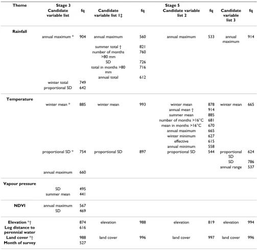
Table 2: Results of bootstrap step-wise procedures. Variables included in the candidate lists of Stage 3 and Stage 5, and their selection frequency (fq), in four separate automated stepwise backward variable exclusion procedures, each time against 1000 bootstrap samples of the malaria prevalence data.
Theme Stage 3 Stage 5
Candidate variable list
fq Candidate
variable list 1‡
fq Candidate variable
list 2
fq Candidate
variable list 3
fq
Rainfall
annual maximum * 904 annual maximum 560 annual maximum 533 annual maximum
914
summer total † 821 number of months
>80 mm
760
SD 726
total in months >80 mm
716
annual total 612 winter total 749
proportional SD 642
Temperature
winter mean * 885 winter mean 993 winter mean 878 winter mean 665 annual mean † 914
summer mean 885 number of months >16°C 681 mean in months >16°C 670 annual maximum 665 winter minimum 627 effective 615 annual minimum 558
proportional SD * 754 proportional SD 897 proportional SD 544 proportional SD
624
SD 786 annual range 537 annual maximum 660
Vapour pressure
SD 495 summer mean 441
NDVI annual maximum 567 SD 469
Elevation *† 874 elevation 988 elevation 819 elevation 994
Log distance to perennial water
616
Land cover *† 988 land cover 996 land cover 997 land cover 996
Month of survey 527
NDVI – normalized difference vegetation index; SD – standard deviation * Variables selected into Stage 4 model
† Variables selected into Stage 5 model
International Journal of Health Geographics 2007, 6:44 http://www.ij-healthgeographics.com/content/6/1/44
Page 9 of 15 (page number not for citation purposes) in the Stage 5 model to four. Results of the Stage 5 model
are shown in table 3.
Figure 6 shows the scatter plot of observed versus predicted logit(p), for the derivation and validation data of the non-spatial Stage 5 model. The concordance correlation coeffi-cient (ρC) [27,28] for the derivation data, weighted by
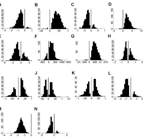
Distribution of coefficients of fourteen candidate variables in 1000 stepwise bootstrap models
Figure 5
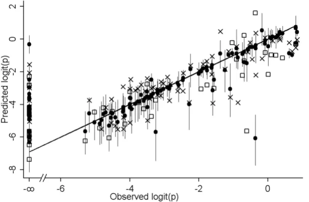
sample size, was 0.851, n (individuals examined) = 11182 in 66 non-zero prevalence surveys, the 95% confidence interval (CI) = 0.846 to 0.856. The unweighted ρC = 0.834, n = 66, CI = 0.760 to 0.908. For the validation data weighted ρC = 0.835, n = 4467, CI = 0.826 to 0.843; unweighted ρC = 0.776, n = 30, CI = 0.635 to 0.917. The difference between observed and predicted logit(p) did not vary with prevalence.
After adjusting for spatial random effects, only three covariates remained significant. Land cover (median = -0.515; 95% CI = -1.099 and 0.059) was removed. The pre-dictions (median and CI) from the spatial Stage 6 model are also shown in figure 6. It contained three co-variates namely summer rainfall, annual mean temperature and elevation, each independently significantly associated with prevalence of infection after allowing for spatial cor-relation in the data (table 4).
Discussion
This study was concerned with finding the best predictors of malaria prevalence in terms of plausibility, parsimony and reliability. One important question was how to sum-marize the environmental data in a meaningful way. We determined to explore a range of alternative summaries of the monthly climate data, believing one appropriate sum-mary indicator to be better for prediction than individual months [5], quarterly aggregates [3], or principal compo-nents [4], the last of which are difficult to interpret. How-ever, as more and more variables are tested against a certain data set, the risk increases that some will explain the data merely by chance, but will fail to explain new data.
In an initial attempt to derive a well-fitting and plausible model through automated step-wise variable selection (results not shown), arbitrary factors such as entry and removal threshold settings, how many variables were
Predicted versus observed prevalence
Figure 6
Predicted versus observed prevalence. Predicted versus observed prevalence, on a logit scale, for the derivation (crosses) and validation (squares) data of the Stage 5 non-spatial model, and for the median (closed circles) and upper/lower confidence interval (spikes) of the Stage 6 spatial model.
Table 3: Results of the Stage 5 non-spatial model. Odds ratios, z-scores, and confidence interval estimated from non-spatial regression against four variables, fitted on derivation data only (n = 81, AIC = 8.06).
Variable Odds Ratio z p(z) 95%confidence interval
lower upper
International Journal of Health Geographics 2007, 6:44 http://www.ij-healthgeographics.com/content/6/1/44
Page 11 of 15 (page number not for citation purposes) included in the list of candidates, and which data-subset
was used for model derivation, affected which variables got selected. The best-fitting models did not produce the most plausible risk maps, and visa versa. The majority of maps resulting from these models strongly contradicted expert opinion. A more systematic selection procedure was called for.
Identification of consistent predictors is compromised by correlation among predictors. A strong, reliable predictor
may ultimately be selected less frequently than a weaker predictor, if several strongly correlated alternatives com-pete for entry into the model so that each has a low selec-tion frequency [11]. For this reason it was important to include in the candidate list only little-correlated varia-bles. This was ensured in Stage 2, where the candidate list was reduced from 42 to 14.
Reliable predictors would not only explain a particular data set, but would be associated consistently with the
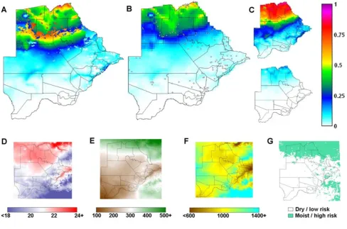
Maps of predicted malaria prevalence and covariates
Figure 7
Maps of predicted malaria prevalence and covariates. Predicted pre-control childhood malaria prevalence maps for Botswana, resulting from (A) the stage 5 non-spatial model and (B) the stage 6 spatial model; 118 survey sites are shown; (C) the upper and lower 95% CI of the spatial model. Co-variates used in the models: (D) annual mean temperature, C; (E) sum-mer total rainfall, mm; (F) elevation, m; (G) land cover categories, high-risk/low-risk. Lines represent district boundaries.
Table 4: Results of the Stage 6 spatial model. Odds ratios and confidence interval estimated from Stage 6 spatial model, fitted on all prevalence data (n = 122).
Variable Odds Ratio 95%confidence interval
lower upper
rainfall summer total (per 100 mm) 2.01 1.49 2.70 temperature annual mean (per °C) 5.75 4.14 8.08
elevation (per 100 m) 1.82 1.49 2.22
response. The bootstrapping of Stage 3 helped identify such predictors, because those that consistently explain different sub-sets of the data, are more likely to explain new data. In the step-wise bootstrap procedures, variables that explained the most observations would be selected most frequently while those that explained only some of the observations, would be selected only when these observations appeared in the bootstrap sample. The effect of individual observations on variable selection, espe-cially of outliers, was thus reduced.
In the process of uni-variate ranking (Stage 1 and 2) we became guilty of "data peeking" [9]. Using our data to assemble a candidate list of predictors set up the analysis for success. Such undeclared testing and discarding of var-iables may lead to illegitimately high model fit. Another problem of Stage 2 was that variables were excluded on the grounds of low uni-variate correlation with the response, while their predictive power may be quite differ-ent once other variables are accounted for. Stage 5 was an attempt to redress both these problems at once, by giving each variable excluded in Stage 2, whose relative had sur-vived up to Stage 4, a fair chance to out-perform and sup-plant its competitors in a multiple-variable context, at the same time, through the bootstrap sub-sampling, to reduce the influence of the data set on this process.
A further benefit of the Stage 3 bootstrap-stepwise proce-dures was the information provided by the frequency dis-tributions of coefficients in the 1000 stepwise models (figure 5). A variable that has a widely varying coefficient, or one that is sometimes positive and sometimes negative, is clearly not reliable and should be considered with sus-picion [33]. An example was summer vapour pressure, the strongest uni-variate predictor, but selected least fre-quently in multiple-variable regression (figure 5J ). Alti-tude on the other hand, a weak uni-variate predictor, became an important predictor in a multiple-variable context, with a stable positive coefficient (figure 5G ). In fact, the most frequently selected variables (table 2) had stable coefficients (figure 5), whereas the most unstable coefficients were found among the least frequently selected variables, confirming the relative importance of predictors.
The strong association found between malaria prevalence and selected environmental data (figure 7) is biologically plausible since high malaria infections have been shown to coincide with conditions that favour vector and para-site development in a given location [3]. However, over small distances environmental conditions vary only slightly due to the relatively simple flat Botswanan topog-raphy, while malaria prevalence showed substantial local variation, for example contemporal measures of 67% (n = 48, Maun) versus 24% (n = 557, Maun suburb), or 3% (n
= 219) versus 17% (n = 116) in Matangwane. Such local variation is perhaps partly caused by the distribution of small breeding sites. Yet in studies where detailed breed-ing site information was available, much of the variation in incidence [34], prevalence and entomologic inocula-tion rate [35] nevertheless remained unexplained. Local-ized factors, such as individual, household and village characteristics, as well as the effect of sampling procedure and size, may further contribute to the unexplained varia-bility in prevalence.
Summer rainfall and annual mean temperature, retained in the final multiple-variable model, were highly plausi-ble predictors. The same variaplausi-bles – summer rain and mean temperature over the preceding year – were also found to explain inter-seasonal variation in malaria inci-dence in KwaZulu-Natal [36]. Summer rainfall also explained much of the variation in inter-annual variation in malaria incidence in Botswana [16]. High rainfall dur-ing the hot summer months allows rapid breeddur-ing and population expansion of the mosquito vectors, while high mean temperatures maximize the maturation rate of the parasite in its exothermic arthropod host [37]. Warmer winters reduce the die-back of mosquitoes and parasites, thereby increasing the reservoir for the following season.
The strong positive association of elevation with malaria prevalence (an increase in logit(p) of 1 every 160 m, table 4) was surprising, as prevalence on its own, as it usually tends to be, was higher in low-lying areas (figure 4G). This positive association was difficult to explain, but may be connected with the malaria control that was ongoing at the time. It appears from early reports [15] that vector control operations were wide-spread and intensive along rivers and the main populated areas.
The non-spatial model of Stage 5 predicted the data fairly well but the predictions achieved by the spatial model of Stage 6 were more accurate (figure 6). The map corre-sponding to the Stage 5 model (figure 7A) had an implau-sible discontinuity, caused by the negative co-efficient of land-cover. Land-cover was the most frequently selected variable in the bootstrap procedures, but was not signifi-cant in the spatial model. This binary variable may simply have approximated the spatial division between high and low prevalence areas, which was ultimately described more correctly through the geo-spatial approach of Stage 6 (figure 7B).
International Journal of Health Geographics 2007, 6:44 http://www.ij-healthgeographics.com/content/6/1/44
Page 13 of 15 (page number not for citation purposes) than the predictions based on environmental factors. By
1961/2 malaria prevalence in the North of Botswana was already much below the level measured in 1944 [14], probably due to the limited use of indoor residual spray-ing which had been ongospray-ing since the 1940's. This high-lights the fact that not only environmental, but also anthropogenic factors, especially malaria control need to be considered. This furthermore highlights the need to monitor control coverage and effectiveness, as well as other potential cofactors, in order to understand the situ-ation more accurately.
Evidence from elsewhere in Africa suggests that prevalence rates in the dry/low transmission season may differ sub-stantially from those in the wet/high transmission season [38,39]. In this study month of survey was a significant predictor of prevalence in a univariate setting only, but not while accounting for other variables. Prevalence by month (figure 4N) was confounded by where surveys were carried out when, and thus did not reflect the season-ality of malaria risk. The highest incidence months for example (March to May) would not be the lowest preva-lence months, as figure 4N suggests. Rather, surveys were carried out during these months in the low-risk South (fig-ure 2). To meas(fig-ure intra-annual variation in prevalence we would have required data from the same localities in different months.
The spatial risk map (figure 7B) presents a smoothed pic-ture of malaria risk in Botswana prior to intensive malaria control, which was highly plausible based on expert opin-ion and the mean incidence at district level [40]. The wide CI (figure 7C) in predicted prevalence highlights the uncertainty remaining after accounting for all explained variation in the data. The confidence level needs to be taken into account when using the map for planning and evaluating control interventions, to avoid over-interpreta-tion of the map.
Conclusion
A continuous map of malaria risk is more useful than point-prevalence rates for several reasons. First, the varia-bility in individual observations may hide underlying pat-terns that have epidemiological importance. Further, it is not possible to deduce from a point-referenced map what prevalence you may expect to see in areas that have not been sampled, whereas a model such as the one devel-oped here gives a likely range of prevalence for the entire region. A continuous prevalence map can also be com-bined with underlying population data to estimate the number of people at risk of – or infected with – malaria. Finally, the spatial statistical methods employed here dis-tinguish between the correlation among observations that can be ascribed to their spatial proximity (neighbouring villages affecting each other), and that which can be
explained by environmental factors (thereby avoiding overestimating the explanatory power of the covariates).
Though malaria risk has been reduced substantially through intense malaria control, a malaria risk map nev-ertheless remains highly useful from the control perspec-tive in knowing historical prevalence levels. We have furthermore demonstrated a systematic procedure for var-iable selection and model formulation in developing a geo-statistical risk model from point-referenced malaria prevalence data, which has relevance to a broad range of environmentally determined infectious diseases. The fail-ure take account of spatial correlations during the entire variable selection procedure remained a major weakness. As computing power increases and statistical software packages are further developed, variable selection within a spatial framework may end up being within the means of the average researcher.
The staged process of variable elimination employed here proved to be practical, though not necessarily the optimal solution. Stepwise variable selection on multiple boot-strap samples drawn from the data allowed us to identify the most consistent and stable explanatory variables. Selection frequency provided an objective rationale for choosing one variable above another, and to choose between similar and strongly correlated indicators. Spatial analysis was the final stage in the variable elimination process, after which we remained with a parsimonious, highly plausible model, which produced a smooth, plau-sible map of malaria risk.
Appendix 1
Standard deviation (SD)
where ym = monthly value and = mean of all ym.
Proportional SD (based on monthly proportions)
where pym = ym/ytot; ytot = ∑ym, and 0.0833 is the mean of all pym (= 1/12)
Effective temperature [41]
Effective temperature = [8 * annual mean + 14 * annual range]/[8 + annual range]
SD= −
=
∑
(y ym)m
2
1 12
ˆy
Proportional SD= −
=
∑
( .0 0833 )21 12
Concentration of rainfall
Monthly rainfall is expressed as a vector (rm, θm), rainfall being the magnitude (r) of the vector and the month its angle (θ) expressed in units of arc:
θm = m2π/12
where m is the month, so that January = 1 and December = 12.
The twelve monthly vectors are added to calculate the total vector (rt, θt):
The concentration index C is calculated as:
C = 100rt/annual total
Concentration is 100% if all the rain falls in one month and 0% if all months have equal amount of rain.
θt is the mean peak month around which rainfall is con-centrated.
Generalized spatial logistic regression analysis
Bayesian geostatistical model formulation has been described by a number of authors [29-32]. Following these authors, the model is specified as follows:
Yji represents the binary response corresponding to the infection status of child j at site i (the survey site) taking value 1 if the child tested positive and 0 otherwise. The Yji
are conditionally independent Bernoulli variables with infection probability pi at location i.
The pi are defined via a generalised linear mixed model, to take account of spatial dependence:
logit(pi) = Xiβ+S(ᐍi)
where βrepresents the regression coefficients for a set of known covariates X at all locations ᐍi of the study area;
S = (S(ᐍ1),...., S(ᐍn))T denotes the values of the
(unob-served) Gaussian spatial process S(·) at sample locations ᐍi;
σ2 = Var{S(ᐍ)}, and Φ is a parameter of the correlation
function ρ(dij, Φ), in our case exp(-dij/Φ), where dij is the distance between locations ᐍi and ᐍj.
For β flat priors were specified respectively (defaults in geoRglm) and for σ2 a Scaled-Inverse chisquare
distribu-tion(χ2
ScI) with five degrees of freedom and a mean of 0.5.
For Φ a discrete exponential prior with mean of 0.04 and 1000 discretisation points in the interval 0.0001 to 2 was specified.
Convergence was assessed by inspecting plots of traces of simulations for individual parameters. The first 50,000 iterations were discarded; thereafter simulations were run for 250,000 iterations. Every 50th sample was retained. For each model parameter the median and 2.5 and 97.5 percentiles were calculated from the 5,000 MCMC simu-lations.
Models were compared by calculating the deviance infor-mation criterion (DIC) for each model [42]. Spatial pre-diction using Bayesian kriging was carried out for a grid of 2300 locations which correspond to the entire surface of Botswana. For each prediction location a posterior sample of MCMC simulations was generated taking account of the estimates of regression coefficients and the spatial effects at each location, and of the uncertainty of each parameter. This process is described in detail elsewhere [29,31,32], and was carried out using geoR [30].
Abbreviations
CI Confidence interval/credible interval
logit(p) Logit-transformed malaria prevalence
MCMC Markov Chain Monte Carlo
NDVI Normalized difference vegetation index
SD Standard deviation
Competing interests
The author(s) declare that they have no competing inter-ests.
Authors' contributions
All authors critically reviewed several versions of the man-uscript. MC carried out the bulk of the analysis and drafted the manuscript. IK participated in its design, car-ried out the spatial analysis and helped draft the manu-script. MM collated the malaria data. MC, IK and MM read and approved the final manuscript. BS recently passed away and we hereby wish to express our deepest appreci-ation of his leadership, his personal and professional
sup-rt rm m r
m
m m
m
=
∑
= cosθ + ∑
= sinθ International Journal of Health Geographics 2007, 6:44 http://www.ij-healthgeographics.com/content/6/1/44
Page 15 of 15 (page number not for citation purposes) port over the years and his tireless efforts towards malaria
control.
Acknowledgements
We thank the Botswana Ministry of Health for contributing their data to the efforts of the MARA project. We acknowledge Tom Smith and Pene-lope Vounatsou of the Swiss Tropical Institute for revising the manuscript critically for important intellectual content and thank them for their valua-ble comments. We thank the South African Medical Research Council and the Rudolf Geigy Stiftung zu Gunsten des Schweizerischen Tropeninstituts for supporting this study, as well as the various funders of the larger MARA project (particularly MIM/TDR and RBM).
References
1. Snow RW, Marsh K, Le Sueur D: The need for maps of transmis-sion intensity to guide malaria control in Africa. Parasitol Today
1996, 12:455-457.
2. Kleinschmidt I, Bagayoko M, Clarke GP, Craig M, Le Sueur D: A spa-tial statistical approach to malaria mapping. Int J Epidemiol
2000, 29:355-361.
3. Kleinschmidt I, Omumbo J, Briet O, Van De GN, Sogoba N, Mensah NK, Windmeijer P, Moussa M, Teuscher T: An empirical malaria distribution map for West Africa. Trop Med Int Health 2001, 6:779-786.
4. Omumbo JA, Hay SI, Snow RW, Tatem AJ, Rogers DJ: Modelling malaria risk in East Africa at high-spatial resolution. Trop Med Int Health 2005, 10:557-566.
5. Snow RW, Gouws E, Omumbo JA, Rapuoda B, Craig MH, Tanser FC, Le Sueur D, Ouma J: Models to predict the intensity of
Plasmo-dium falciparum transmission: applications to the burden of
disease in Kenya. Trans R Soc Trop Med Hyg 1998, 92:601-606. 6. Gemperli A, Vounatsou P, Sogoba N, Smith T: Malaria mapping
using transmission models: application to survey data from Mali. Am J Epidemiol 2006, 163:289-297.
7. Justice AC, Covinsky KE, Berlin JA: Assessing the generalizability of prognostic information. Ann Intern Med 1999, 130:515-524. 8. Diggle P, Moyeed R, Rowlingson B, Thomson M: Childhood
malaria in the Gambia: a case-study in model-based statis-tics. Applied Statistics 2002, 51:493-506.
9. Babyak MA: What you see may not be what you get: a brief, nontechnical introduction to overfitting in regression-type models. Psychosom Med 2004, 66:411-421.
10. Harrell FE Jr: Regression modeling strategies: with applications to linear models, logistic regression and survival analysis New York: Springer; 2001.
11. Austin PC, Tu JV: Bootstrap methods for developing predictive models. Am Stat 2004, 58:131-137.
12. Deichmann U: Population Density for Africa in 1990, 3. Internet
1997 [http://grid.cr.usgs.gov/datasets/mapservices.php]. NCGIA, UCSB, Santa Barbara
13. Chayabejara S, Sobti SK, Payne D, Braga F: Malaria situation in Botswana. In Report AFR/MAL/144 World Health Organization, Regional Office for Africa.
14. Mabaso ML, Sharp B, Lengeler C: Historical review of malarial control in southern African with emphasis on the use of indoor residual house-spraying. Trop Med Int Health 2004, 9:846-856.
15. Freedman ML: Malaria Control. In Report The Botswana National Archives and Records Services, Gaborone.
16. Thomson MC, Mason SJ, Phindela T, Connor SJ: Use of rainfall and sea surface temperature monitoring for malaria early warn-ing in Botswana. Am J Trop Med Hyg 2005, 73:214-221.
17. Omumbo J, Ouma J, Rapuoda B, Craig MH, Le Sueur D, Snow RW: Mapping malaria transmission intensity using geographical information systems (GIS): an example from Kenya. Ann Trop Med Parasitol 1998, 92:7-21.
18. Anon: Stata Statistical Software: Release 7.0. Stata Corpora-tion, College StaCorpora-tion, Texas; 2001.
19. Anon: GTOPO30 global digital elevation model. Internet 1998 [http://edc.usgs.gov/products/elevation/gtopo30/gtopo30.html]. Center for Earth Resources Observation and ScienceUnited States Geological Survey, Sioux Falls, South Dakota
20. Anon: Africa Data Sampler, 1. In CD-ROM World Resources Insti-tute, Washington, DC; 1995.
21. Anderson JR, Hardy EE, Roach JT, Witmer RE: A land use and land cover classification system for use with remote sensor data.
U S Geological Survey Professional Paper 1976, 964:.
22. Hutchinson MF, Nix HA, McMahan JP, Ord KD: Africa – A topo-graphic and climatic database, 1. CD-ROM, Canberra 1995. 23. Mitchell TD, Hulme M, New M: CRU TS 2.0 high-resolution
grid-ded climate data, 1. Internet 2003 [http://www.cru.uea.ac.uk/cru/ data/hrg.htm]. Climate Research Unit, University of East Anglia, Nor-wich.
24. Anon: Pathfinder Advanced Very High Resolution Radiome-ter (AVHRR) data. Internet 2001 [http://daac.gsfc.nasa.gov/data/ dataset/]. National Oceanic and Atmospheric Administration (NOAA), Goddard Distributed Active Archive Center
25. Anon: Global Land 1-KM AVHRR Project. Internet 2007 [http:// edcsns17.cr.usgs.gov/1KM/1kmhomepage.html]. Center for Earth Resources Observation and Science, United States Geologic Survey, Sioux Falls
26. Akaike H: Information theory and an extension of the maxi-mum likelihood principle. In Second international symposium on information theory Edited by: Petrov BN, Csaki F. Budapest: Akademiai Kiado; 1973:267-281.
27. Lin LIK: A concordance correlation coefficient to evaluate reproducibility. Biometrics 1989, 45:255-268.
28. Lin LIK: A note on the concordance correlation coefficient.
Biometrics 2000, 56:324-325.
29. Diggle PJ, Tawn JA, Moyeed R: Model-based geostatistics. J Roy Stat Soc C 1998, 47:299-350.
30. Christensen OF, Ribeiro PJJ: geoRglm – a package for general-ised linear spatial models. R News 2002, 2:26-28.
31. Gemperli A, Vounatsou P: Fitting generalized linear mixed models for point-referenced spatial data. J Modern Appl Stat Meth 2003, 2:497-511.
32. Gemperli A, Vounatsou P, Kleinschmidt I, Bagayoko M, Lengeler C, Smith T: Spatial patterns of infant mortality in Mali: the effect of malaria endemicity. Am J Epidemiol 2004, 159:64-72. 33. Concato J, Feinstein AR, Holford TR: The risk of determining risk
with multivariable models. Ann Intern Med 1993, 118:201-210. 34. Van Der Hoek W, Konradsen F, Amerasinghe PH, Perera D,
Piya-ratne M, Amerasinghe FP: Towards a risk map of malaria for Sri Lanka: the importance of house location relative to vector breeding sites. Int J Epidemiol 2003, 32:280-285.
35. Hightower AW, Ombok M, Otieno R, Odhiambo R, Oloo AJ, Lal AA, Nahlen BL, Hawley WA: A geographic information system applied to a malaria field study in western Kenya. Am J Trop Med Hyg 1998, 58:266-272.
36. Craig MH, Kleinschmidt I, Nawn JB, Le Sueur D, Sharp BL: Exploring 30 years of malaria case data in KwaZulu-Natal, South Africa, Part I: the impact of climatic factors. Trop Med Int Health 2004, 9:1247-1257.
37. Molineaux L: The epidemiology of human malaria as an expla-nation of its distribution, including some implications for its control. In Malaria: Principles and Practice of MalariologyVolume 2. Edited by: Wernsdorfer WH, McGregor I. Edinburgh: Churchill Liv-ingstone; 1988:913-998.
38. Lindsay SW, Wilkins HA, Zieler HA, Daly RJ, Petrarca V, Byass P: Ability of Anopheles gambiae mosquitoes to transmit malaria during the dry and wet seasons in an area of irrigated rice cultivation in The Gambia. J Trop Med Hyg 1991, 94:313-324.
39. Molineaux L, Gramiccia G: The Garki project: research on the epidemiol-ogy and control of malaria in the Sudan savanna of West Africa Geneva: World Health Organization; 1980.
40. Craig MH, Snow RW, Le Sueur D: A climate-based distribution model of malaria transmission in Africa. Parasitol Today 1999, 15:105-111.
41. Stuckenberg BR: Effective temperature as an ecological factor in southern Africa. Zool Afr 1969, 4:145-197.