Learning Multi-modal Similarity

(1)

Learning Multi-modal Similarity

Brian McFee [email protected]

Department of Computer Science and Engineering University of California

San Diego, CA 92093-0404, USA

Gert Lanckriet [email protected]

Department of Electrical and Computer Engineering University of California

San Diego, CA 92093-0407, USA

Editor: Tony Jebara

Abstract

In many applications involving multi-media data, the definition of similarity between items is inte-gral to several key tasks, including nearest-neighbor retrieval, classification, and recommendation. Data in such regimes typically exhibits multiple modalities, such as acoustic and visual content of video. Integrating such heterogeneous data to form a holistic similarity space is therefore a key challenge to be overcome in many real-world applications.

We present a novel multiple kernel learning technique for integrating heterogeneous data into a single, unified similarity space. Our algorithm learns an optimal ensemble of kernel transfor-mations which conform to measurements of human perceptual similarity, as expressed by relative comparisons. To cope with the ubiquitous problems of subjectivity and inconsistency in multi-media similarity, we develop graph-based techniques to filter similarity measurements, resulting in a simplified and robust training procedure.

Keywords: multiple kernel learning, metric learning, similarity

1. Introduction

(2)

Without extra information to guide the construction of a similarity measure, the situation seems hopeless. However, if some side-information is available, for example, as provided by human label-ers, it can be used to formulate a learning algorithm to optimize the similarity measure.

This idea of using side-information to optimize a similarity function has received a great deal of attention in recent years. Typically, the notion of similarity is captured by a distance metric over a vector space (e.g., Euclidean distance inRd), and the problem of optimizing similarity reduces to finding a suitable embedding of the data under a specific choice of the distance metric. Metric

learn-ing methods, as they are known in the machine learnlearn-ing literature, can be informed by various types

of side-information, including class labels (Xing et al., 2003; Goldberger et al., 2005; Globerson and Roweis, 2006; Weinberger et al., 2006), or binary similar/dissimilar pairwise labels (Wagstaff et al., 2001; Shental et al., 2002; Bilenko et al., 2004; Globerson and Roweis, 2007; Davis et al., 2007). Alternatively, multidimensional scaling (MDS) techniques are typically formulated in terms of quantitative (dis)similarity measurements (Torgerson, 1952; Kruskal, 1964; Cox and Cox, 1994; Borg and Groenen, 2005). In these settings, the representation of data is optimized so that distance (typically Euclidean) conforms to side-information. Once a suitable metric has been learned, sim-ilarity to new, unseen data can be computed either directly (if the metric takes a certain parametric form, for example, a linear projection matrix), or via out-of-sample extensions (Bengio et al., 2004). To guide the construction of a similarity space for multi-modal data, we adopt the idea of using similarity measurements, provided by human labelers, as side-information. However, it has to be noted that, especially in heterogeneous, multi-media domains, similarity may itself be a highly subjective concept and vary from one labeler to the next (Ellis et al., 2002). Moreover, a single labeler may not be able to consistently decide if or to what extent two objects are similar, but she may still be able to reliably produce a rank-ordering of similarity over pairs (Kendall and Gibbons, 1990). Thus, rather than rely on quantitative similarity or hard binary labels of pairwise similarity, it is now becoming increasingly common to collect similarity information in the form of triadic or

relative comparisons (Schultz and Joachims, 2004; Agarwal et al., 2007), in which human labelers

answer questions of the form:

“Is x more similar to y or z?”

Although this form of similarity measurement has been observed to be more stable than quantitative similarity (Kendall and Gibbons, 1990), and clearly provides a richer representation than binary pairwise similarities, it is still subject to problems of consistency and inter-labeler agreement. It is therefore imperative that great care be taken to ensure some sense of robustness when working with perceptual similarity measurements.

In the present work, our goal is to develop a framework for integrating multi-modal data so as to optimally conform to perceptual similarity encoded by relative comparisons. In particular, we follow three guiding principles in the development of our framework:

1. The algorithm should be robust against subjectivity and inter-labeler disagreement.

2. The algorithm must be able to integrate multi-modal data in an optimal way, that is, the distances between embedded points should conform to perceptual similarity measurements.

3. It must be possible to compute distances to new, unseen data as it becomes available.

(3)

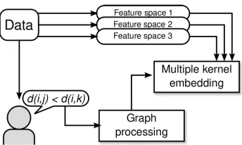
Feature space 1 Feature space 2 Feature space 3

d(i,j) < d(i,k)

Figure 1: An overview of our proposed framework for multi-modal feature integration. Data is represented in multiple feature spaces (each encoded by a kernel function). Humans supply perceptual similarity measurements in the form of relative pairwise comparisons, which are in turn filtered by graph processing algorithms, and then used as constraints to optimize the multiple kernel embedding.

the data that optimally reproduces the similarity measurements. This type of embedding problem has been previously studied by Agarwal et al. (2007) and Schultz and Joachims (2004). However, Agarwal et al. (2007) provide no out-of-sample extension, and neither support heterogeneous feature integration, nor do they address the problem of noisy similarity measurements.

A common approach to optimally integrate heterogeneous data is based on multiple kernel

learning, where each kernel encodes a different modality of the data. Heterogeneous feature

inte-gration via multiple kernel learning has been addressed by previous authors in a variety of contexts, including classification (Lanckriet et al., 2004; Zien and Ong, 2007; Kloft et al., 2009; Jagarlapudi et al., 2009), regression (Sonnenburg et al., 2006; Bach, 2008; Cortes et al., 2009), and dimension-ality reduction (Lin et al., 2009). However, none of these methods specifically address the problem of learning a unified data representation which conforms to perceptual similarity measurements.

1.1 Contributions

Our contributions in this work are two-fold. First, we develop the partial order embedding (POE) framework (McFee and Lanckriet, 2009b), which allows us to use graph-theoretic algorithms to filter a collection of subjective similarity measurements for consistency and redundancy. We then formulate a novel multiple kernel learning (MKL) algorithm which learns an ensemble of feature space projections to produce a unified similarity space. Our method is able to produce non-linear embedding functions which generalize to unseen, out-of-sample data. Figure 1 provides a high-level overview of the proposed methods.

(4)

perception measurements. Finally, we prove hardness of dimensionality reduction in this setting in Section 6, and conclude in Section 7.

1.2 Preliminaries

A (strict) partial order is a binary relation R over a set Z (R_⊆Z2) which satisfies the following properties:1

• Irreflexivity:(a,a)_∈/R,

• Transitivity:(a,b)_∈R_∧(b,c)_∈R_⇒(a,c)_∈R,

• Anti-symmetry:(a,b)_∈R_⇒(b,a)_∈/R.

Every partial order can be equivalently represented as a directed acyclic graph (DAG), where each vertex is an element of Z and an edge is drawn from a to b if(a,b)_∈R. For any partial order, R

may refer to either the set of ordered tuples_{(a,b)_}or the graph (DAG) representation of the partial order; the use will be clear from context.

For a directed graph G, we denote by G∞its transitive closure, that is, G∞contains an edge(i,j)

if and only if there exists a path from i to j in G. Similarly, the transitive reduction (denoted Gmin₎

is the minimal graph with equivalent transitivity to G, that is, the graph with the fewest edges such that Gmin∞=G∞.

Let

X

=_{x1,x2, . . . ,xn}denote the training set of n items. A Euclidean embedding is a function

g :

X

_→_Rd _{which maps}

_X

_{into a d-dimensional space equipped with the Euclidean (}_ℓ

2) metric: kx₋y_k2=

q

(x₋y)T₍_x₋_y₎_.

For any matrix B, let Bi denote its ith column vector. A symmetric matrix A∈Rn×n has a spectral decomposition A=VΛVT, whereΛ=diag(λ1,λ2, . . . ,λn)is a diagonal matrix containing the eigenvalues of A, and V contains the eigenvectors of A. We adopt the convention that eigenvalues (and corresponding eigenvectors) are sorted in descending order. A is positive semi-definite (PSD), denoted by A0, if each eigenvalue is non-negative:λi≥0,i=1, . . . ,n. Finally, a PSD matrix A gives rise to the Mahalanobis distance function

kx₋y_kA=

q

(x₋y)T_A₍_x₋_y₎_.

2. A Graphical View of Similarity

Before we can construct an embedding algorithm for multi-modal data, we must first establish the form of side-information that will drive the algorithm, that is, the similarity measurements that will be collected from human labelers. There is an extensive body of work on the topic of constructing a geometric representation of data to fit perceptual similarity measurements. Primarily, this work falls under the umbrella of multi-dimensional scaling (MDS), in which perceptual similarity is modeled by numerical responses corresponding to the perceived “distance” between a pair of items, for

(5)

example, on a similarity scale of 1–10. (See Cox and Cox 1994 and Borg and Groenen 2005 for comprehensive overviews of MDS techniques.)

Because “distances” supplied by test subjects may not satisfy metric properties—in particular, they may not correspond to Euclidean distances—alternative non-metric MDS (NMDS) techniques have been proposed (Kruskal, 1964). Unlike classical or metric MDS techniques, which seek to preserve quantitative distances, NDMS seeks an embedding in which the rank-ordering of distances is preserved.

Since NMDS only needs the rank-ordering of distances, and not the distances themselves, the task of collecting similarity measurements can be simplified by asking test subjects to order pairs of points by similarity:

“Are i and j more similar than k andℓ?”

or, as a special case, the “triadic comparison”

“Is i more similar to j orℓ?”

Based on this kind of relative comparison data, the embedding problem can be formulated as fol-lows. Given is a set of objects

X

, and a set of similarity measurements

C

=_{(i,j,k, ℓ)_{} ⊆}

X

4_,

where a tuple(i,j,k, ℓ)is interpreted as “i and j are more similar than k andℓ.” (This formulation subsumes the triadic comparisons model when i=k.) The goal is to find an embedding function g :

X

_→_Rd _{such that}

∀(i,j,k, ℓ)_∈

C

: _kg(i)₋g(j)_k2+1<_kg(k)₋g(ℓ)_k2. (1) The unit margin is forced between the constrained distances for numerical stability.

Agarwal et al. (2007) work with this kind of relative comparison data and describe a generalized NMDS algorithm (GNMDS), which formulates the embedding problem as a semi-definite program. Schultz and Joachims (2004) derive a similar algorithm which solves a quadratic program to learn a linear, axis-aligned transformation of data to fit relative comparisons.

Previous work on relative comparison data often treats each measurement(i,j,k, ℓ)_∈

C

as ef-fectively independent (Schultz and Joachims, 2004; Agarwal et al., 2007). However, due to their semantic interpretation as encoding pairwise similarity comparisons, and the fact that a pair(i,j)

may participate in several comparisons with other pairs, there may be some global structure to

C

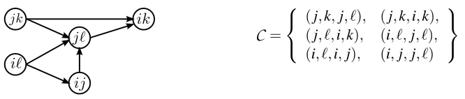
which these previous methods are unable to exploit.

In Section 2.1, we develop a graphical framework to infer and interpret the global structure exhibited by the constraints of the embedding problem. Graph-theoretic algorithms presented in Section 2.2 then exploit this representation to filter this collection of noisy similarity measurements for consistency and redundancy. The final, reduced set of relative comparison constraints defines a partial order, making for a more robust and efficient embedding problem.

2.1 Similarity Graphs

To gain more insight into the underlying structure of a collection of comparisons

C, we can represent

C

as a directed graph over

X

2_{. Each vertex in the graph corresponds to a pair}₍_i,_j₎_∈

_X

2_{, and an edge}

(6)

C

=

  

(j,k,j, ℓ), (j,k,i,k), (j, ℓ,i,k), (i, ℓ,j, ℓ), (i, ℓ,i,j), (i,j,j, ℓ)

  

Figure 2: The graph representation (left) of a set of relative comparisons (right).

1. If

C

contains cycles, then there exists no embedding which can satisfy

C

.

2. If

C

is acyclic, any embedding that satisfies the transitive reduction

C

min_{also satisfies}

_C

_.

The first fact implies that no algorithm can produce an embedding which satisfies all measure-ments if the graph is cyclic. In fact, the converse of this statement is also true: if

C

is acyclic, then an embedding exists in which all similarity measurements are preserved (see Appendix A). If

C

is cyclic, however, by analyzing the graph, it is possible to identify an “unlearnable” subset of

C

which must be violated by any embedding.

Similarly, the second fact exploits the transitive nature of distance comparisons. In the example depicted in Figure 2, any g that satisfies(j,k,j, ℓ)and(j, ℓ,i,k)must also satisfy(j,k,i,k). In effect, the constraint(j,k,i,k)is redundant, and may also be safely omitted from

C

.

These two observations allude to two desirable properties in

C

for embedding methods:

tran-sitivity and anti-symmetry. Together with irreflexivity, these fit the defining characteristics of a partial order. Due to subjectivity and inter-labeler disagreement, however, most collections of

rel-ative comparisons will not define a partial order. Some graph processing, presented next, based on an approximate maximum acyclic subgraph algorithm, can reduce them to a partial order.

2.2 Graph Simplification

Because a set of similarity measurements

C

containing cycles cannot be embedded in any Euclidean space,

C

is inherently inconsistent. Cycles in

C

therefore constitute a form of label noise. As noted by Angelova (2004), label noise can have adverse effects on both model complexity and general-ization. This problem can be mitigated by detecting and pruning noisy (confusing) examples, and training on a reduced, but certifiably “clean” set (Angelova et al., 2005; Vezhnevets and Barinova, 2007).

Unlike most settings, where the noise process affects each label independently—for example, random classification noise (Angluin and Laird, 1988)—the graphical structure of interrelated rel-ative comparisons can be exploited to detect and prune inconsistent measurements. By eliminating similarity measurements which cannot be realized by any embedding, the optimization procedure can be carried out more efficiently and reliably on a reduced constraint set.

Ideally, when eliminating edges from the graph, we would like to retain as much information as possible. Unfortunately, this is equivalent to the maximum acyclic subgraph problem, which is NP-Complete (Garey and Johnson, 1979). A1_/2_{-approximate solution can be achieved by a simple}

greedy algorithm (Algorithm 1) (Berger and Shor, 1990).

(7)

Algorithm 1 Approximate maximum acyclic subgraph (Aho et al., 1972) Input: Directed graph G= (V,E)

Output: Acyclic graph G′ E′_← /0

for each(u,v)_∈E in random order do if E′_{∪ {}(u,v)_}is acyclic then

E′←E′∪ {(u,v)_} end if

end for G′←(V,E′)

By filtering the constraint set for consistency, we ensure that embedding algorithms are not learning from spurious information. Additionally, pruning the constraint set by transitive reduc-tion focuses embedding algorithms on the most important core set of constraints while reducing overhead due to redundant information.

3. Partial Order Embedding

Now that we have developed a language for expressing similarity between items, we are ready to formulate the embedding problem. In this section, we develop an algorithm that learns a represen-tation of data consistent with a collection of relative similarity measurements, and allows to map unseen data into the learned similarity space after learning. In order to accomplish this, we will assume a feature representation for

X

. By parameterizing the embedding function g in terms of the feature representation, we will be able to apply g to any point in the feature space, thereby generalizing to data outside of the training set.

3.1 Linear Projection

To start, we assume that the data originally lies in some Euclidean space, that is,

X

_⊂_RD_{. There are} of course many ways to define an embedding function g :RD_→_Rd_{. Here, we will restrict attention} to embeddings parameterized by a linear projection matrix M, so that for a vector x_∈RD,

g(x)=. Mx.

Collecting the vector representations of the training set as columns of a matrix X_∈RD×n, the inner product matrix of the embedded points can be characterized as

A=XTMTMX.

Now, for a relative comparison (i,j,k, ℓ), we can express the distance constraint (1) between embedded points as follows:

(Xi−Xj)TMTM(Xi−Xj) +1≤(Xk−Xℓ)TMTM(Xk−Xℓ).

(8)

constraints by introducing a slack variableξi jkℓ≥0 for each constraint, and minimize the empirical

hinge loss over constraint violations1_/_|C_|∑_Cξ_{i jk}_ℓ. This choice of loss function can be interpreted as a convex approximation to a generalization of the area under an ROC curve (see Appendix C).

To avoid over-fitting, we introduce a regularization term tr(MTM), and a trade-off parameterβ>

0 to control the balance between regularization and loss minimization. This leads to a regularized risk minimization objective:

min

M,ξ≥0 tr(M

T_M_{) +} β

|

C

_|

∑

_C ξi jkℓ (2)

s.t. (Xi−Xj)TMTM(Xi−Xj) +1≤(Xk−Xℓ)TMTM(Xk−Xℓ) +ξi jkℓ,

∀(i,j,k, ℓ)_∈

C

.

After learning M by solving this optimization problem, the embedding can be extended to out-of-sample points x′by applying the projection: x′_7→Mx′.

Note that the distance constraints in (2) involve differences of quadratic terms, and are therefore not convex. However, since M only appears in the form MTM in (2), the optimization problem can

be expressed in terms of a positive semi-definite matrix W=. MTM. This change of variables results

in Algorithm 2, a (convex) semi-definite programming (SDP) problem (Boyd and Vandenberghe, 2004), since objective and constraints are linear in W , including the linear matrix inequality W 0. The corresponding inner product matrix is

A=XTW X.

Finally, after the optimal W is found, the embedding function g :RD_→_RD _{can be recovered} from the spectral decomposition of W :

W=VΛVT _⇒ g(x) =Λ1/2VTx,

and a d-dimensional approximation can be recovered by taking the leading d eigenvectors of W .

Algorithm 2 Linear partial order embedding (LPOE) Input: n objects

X

,

partial order

C,

data matrix X ∈RD×n,

β>0

Output: mapping g :

X

_→_Rd

min

W,ξ tr(W) +

β

|

C

_|

∑

_C ξi jkℓ

d(xi,xj)= (. Xi−Xj)TW(Xi−Xj)

d(xi,xj) +1≤d(xk,xℓ) +ξi jkℓ

ξi jkℓ≥0 ∀(i,j,k, ℓ)∈

C

(9)

3.2 Non-linear Projection via Kernels

The formulation in Algorithm 2 can be generalized to support non-linear embeddings by the use of kernels, following the method of Globerson and Roweis (2007): we first map the data into a reproducing kernel Hilbert space (RKHS)

H

via a feature mapφwith corresponding kernel function

k(x,y) =_hφ(x),φ(y)_iH; then, the data is mapped to Rd by a linear projection M :

H

→Rd. The

embedding function g :

X

_→_Rd_{is the therefore the composition of the projection M with}_φ_:

g(x) =M(φ(x)).

Becauseφmay be non-linear, this allows us to learn a non-linear embedding g.

More precisely, we consider M as being comprised of d elements of

H

, that is,_{ω1,ω2, . . . ,ωd} ⊆

H

. The embedding g can thus be expressed as

g(x) = (_hωp,φ(x)iH)d_p₌₁,

where(_·)d

p=1denotes concatenation.

Note that in general,

H

may be infinite-dimensional, so directly optimizing M may not be feasible. However, by appropriately regularizing M, we may invoke the generalized representer theorem (Schölkopf et al., 2001). Our choice of regularization is the Hilbert-Schmidt norm of M, which, in this case, reduces to

kM_k2_HS=

d

∑

p=1

hωp,ωpiH.

With this choice of regularization, it follows from the generalized representer theorem that at an optimum, eachωpmust lie in the span of the training data, that is,

ωp= n

∑

i=1

Npiφ(xi), p=1, . . . ,d,

for some real-valued matrix N_∈Rd×n. IfΦis a matrix representation of

X

in

H

(i.e.,Φi=φ(xi) for xi∈

X

), then the projection operator M can be expressed as

M=NΦT. (3)

We can now reformulate the embedding problem as an optimization over N rather than M. Using (3), the regularization term can be expressed as

kM_k2_HS=tr(ΦNTNΦT) =tr(NTNΦTΦ) =tr(NTNK),

where K is the kernel matrix over

X

:

K=ΦT_Φ_, _{with K}

i j=hφ(xi),φ(xj)iH =k(xi,xj).

To formulate the distance constraints in terms of N, we first express the embedding g in terms of N and the kernel function:

(10)

where Kx is the column vector formed by evaluating the kernel function k at x against the training set. The inner product matrix of embedded points can therefore be expressed as

A=KNTNK,

which allows to express the distance constraints in terms of N and the kernel matrix K:

(Ki−Kj)TNTN(Ki−Kj) +1≤(Kk−Kℓ)TNTN(Kk−Kℓ).

The embedding problem thus amounts to solving the following optimization problem in N andξ:

min

N,ξ≥0 tr(N

T_NK_{) +} β

|

C

_|

∑

_C ξi jkℓ (4)

s.t. (Ki−Kj)TNTN(Ki−Kj) +1≤(Kk−Kℓ)TNTN(Kk−Kℓ) +ξi jkℓ,

∀(i,j,k, ℓ)_∈

C

.

Again, the distance constraints in (4) are non-convex due to the differences of quadratic terms. And, as in the previous section, N only appears in the form of inner products NTN in (4)—both

in the constraints, and in the regularization term—so we can again derive a convex optimization problem by changing variables to W =. NTN 0. The resulting embedding problem is listed as Algorithm 3, again a semi-definite programming problem (SDP), with an objective function and constraints that are linear in W .

After solving for W , the matrix N can be recovered by computing the spectral decomposition

W=VΛVT, and defining N=Λ1/2_VT_{. The resulting embedding function takes the form:}

g(x) =Λ1/2_VT_K

x.

As in Schultz and Joachims (2004), this formulation can be interpreted as learning a Maha-lanobis distance metric ΦWΦT over

H

. More generally, we can view this as a form of kernel learning, where the kernel matrix A is restricted to the set

A∈ {KW K : W 0}. (5)

3.3 Connection to GNMDS

We conclude this section by drawing a connection between Algorithm 3 and the generalized non-metric MDS (GNMDS) algorithm of Agarwal et al. (2007).

First, we observe that the i-th column, Ki, of the kernel matrix K can be expressed in terms of K and the ithstandard basis vector ei:

Ki=Kei.

From this, it follows that distance computations in Algorithm 3 can be equivalently expressed as

d(xi,xj) = (Ki−Kj)TW(Ki−Kj)

= (K(ei−ej))TW(K(ei−ej))

(11)

Algorithm 3 Kernel partial order embedding (KPOE) Input: n objects

X

,

partial order

C,

kernel matrix K,

β>0

X

_→_Rn

min

W,ξ tr(W K) +

β

|

C

_|

∑

_C ξi jkℓ

d(xi,xj)= (. Ki−Kj)TW(Ki−Kj)

ξi jkℓ≥0 ∀(i,j,k, ℓ)∈

C

W 0

If we consider the extremal case where K=I, that is, we have no prior feature-based knowledge of

similarity between points, then Equation 6 simplifies to

d(xi,xj) = (ei−ej)TIW I(ei−ej) =Wii+Wj j−Wi j−Wji.

Therefore, in this setting, rather than defining a feature transformation, W directly encodes the inner products between embedded training points. Similarly, the regularization term becomes

tr(W K) =tr(W I) =tr(W).

Minimizing the regularization term can be interpreted as minimizing a convex upper bound on the rank of W (Boyd and Vandenberghe, 2004), which expresses a preference for low-dimensional embeddings. Thus, by setting K=I in Algorithm 3, we directly recover the GNMDS algorithm.

Note that directly learning inner products between embedded training data points rather than a feature transformation does not allow a meaningful out-of-sample extension, to embed unseen data points. On the other hand, by Equation 5, it is clear that the algorithm optimizes over the entire cone of PSD matrices. Thus, if

C

defines a DAG, we could exploit the fact that a partial order over distances always allows an embedding which satisfies all constraints in

C

(see Appendix A) to eliminate the slack variables from the program entirely.

4. Multiple Kernel Embedding

(12)

However, by encoding each source of information independently by separate feature spaces

H

1_,

_H

2_{, . . .}_{—equivalently, kernel matrices K}1_,_K2_{, . . .}_{—we can formulate a multiple kernel}

learn-ing algorithm to optimally combine all feature spaces into a slearn-ingle, unified embeddlearn-ing space. In this section, we will derive a novel, projection-based approach to multiple-kernel learning and extend Algorithm 3 to support heterogeneous data in a principled way.

4.1 Unweighted Combination

Let K1,K2_{, . . . ,}_Km_{be a set of kernel matrices, each with a corresponding feature map}φp_{and RKHS}

H

p_{, for p}_∈₁_{, . . . ,}_{m. One natural way to combine the kernels is to look at the product space, which} is formed by concatenating the feature maps:

φ(xi) = (φ1(xi),φ2(xi), . . . ,φm(xi)) = (φp(xi))mp=1.

Inner products can be computed in this space by summing across each feature map:

hφ(xi),φ(xj)i= m

∑

p=1

_φ_p

(xi),φp(xj)

Hp.

resulting in the sum-kernel—also known as the average kernel or product space kernel. The corre-sponding kernel matrix can be conveniently represented as the unweighted sum of the base kernel matrices:

b

K=

m

∑

p=1

Kp. (7)

SinceK is a valid kernel matrix itself, we could useb K as input for Algorithm 3. As a result, theb

algorithm would learn a kernel from the family

K

₁=

(

m

∑

p=1 Kp

!

W

m

∑

p=1 Kp

!

: W 0

)

=

( _m

∑

p,q=1

KpW Kq : W 0 )

.

4.2 Weighted Combination

Note that

K

1treats each kernel equally; it is therefore impossible to distinguish good features (i.e.,

those which can be transformed to best fit

C) from bad features, and as a result, the quality of

the resulting embedding may be degraded. To combat this phenomenon, it is common to learn a scheme for weighting the kernels in a way which is optimal for a particular task. The most common approach to combining the base kernels is to take a positive-weighted sum

m

∑

p=1

µpKp (µp≥0),

where the weights µpare learned in conjunction with a predictor (Lanckriet et al., 2004; Sonnenburg et al., 2006; Bach, 2008; Cortes et al., 2009). Equivalently, this can be viewed as learning a feature map

φ(xi) = √µpφp(xi)

(13)

where each base feature map has been scaled by the corresponding weight√µp.

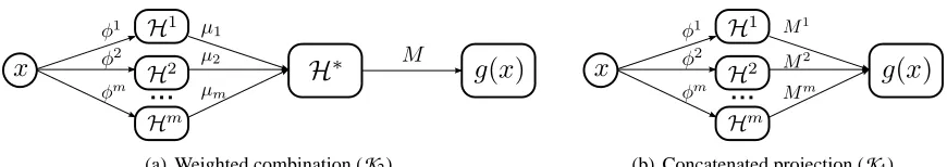
Applying this reasoning to learning an embedding that conforms to perceptual similarity, one might consider a two-stage approach to parameterizing the embedding (Figure 3(a)): first construct a weighted kernel combination, and then project from the combined kernel space. Lin et al. (2009) formulate a dimensionality reduction algorithm in this way. In the present setting, this would be achieved by simultaneously optimizing W and µpto choose an inner product matrix A from the set

K

₂=

( _m

∑

p=1 µpKp

!

W

m

∑

p=1 µpKp

!

: W 0,_∀p, µp≥0

)

=

(

m

∑

p,q=1

µpKpW µqKq : W0,∀p,µp≥0

)

.

The corresponding distance constraints, however, contain differences of terms cubic in the opti-mization variables W and µp:

∑

p,q

K_ip₋K_jpTµpW µq

K_iq₋Kq_j+1_≤

∑

p,q

K_kp₋K_ℓpTµpW µq Kkq−K q

ℓ

,

and are therefore non-convex and difficult to optimize. Even simplifying the class by removing cross-terms, that is, restricting A to the form

K

₃=

( _m

∑

p=1

µ2_pKpW Kp : W0,_∀p,µp≥0

)

,

still leads to a non-convex problem, due to the difference of positive quadratic terms introduced by distance calculations:

m

∑

p=1

K_ip−Kp_j

T

µ2_pW

µpKip−K p j

+1≤

m

∑

p=1

K_kp−K_ℓpTµ2_pW µpK_kp−K_ℓp

.

However, a more subtle problem with this formulation lies in the assumption that a single weight can characterize the contribution of a kernel to the optimal embedding. In general, different kernels may be more or less informative on different subsets of

X

or different regions of the corresponding feature space. Constraining the embedding to a single metric W with a single weight µp for each kernel may be too restrictive to take advantage of this phenomenon.

4.3 Concatenated Projection

We now return to the original intuition behind Equation 7. The sum-kernel represents the inner product between points in the space formed by concatenating the base feature mapsφp. The sets

K

₂ and

K

₃characterize projections of the weighted combination space, and turn out to not be amenable to efficient optimization (Figure 3(a)). This can be seen as a consequence of prematurely combining kernels prior to projection.

(14)

projections, each tailored to its corresponding domain space and jointly optimized to produce an optimal space. By contrast, the previously discussed formulations apply essentially the same pro-jection to each (weighted) feature space, and are thus much less flexible than our proposed approach. Mathematically, an embedding function of this form can be expressed as the concatenation

g(x) = (Mp(φp(x)))m_p₌₁.

Now, given this characterization of the embedding function, we can adapt Algorithm 3 to opti-mize over multiple kernels. As in the single-kernel case, we introduce regularization terms for each projection operator Mp

m

∑

p=1

kMp_k2_HS

to the objective function. Again, by invoking the representer theorem for each Mp, it follows that

Mp=Np(Φp)T,

for some matrix Np_{, which allows to reformulate the embedding problem as a joint optimization over}

Np, p=1, . . . ,m rather than Mp_, _p₌₁_{, . . . ,}_{m. Indeed, the regularization terms can be expressed as}

m

∑

p=1

kMp_k2_HS=

m

∑

p=1

tr(Np)T₍_Np₎_Kp_. ₍₈₎

The embedding function can now be rewritten as

g(x) = (Mp(φp(x)))m_p₌₁= (NpK_xp)m_p₌₁, (9) and the inner products between embedded points take the form:

Ai j =hg(xi),g(xj)i= m

∑

p=1

NpK_ipTNpK_jp

=

m

∑

p=1

(K_ip)T(Np)T(Np)(Kp_j).

Similarly, squared Euclidean distance also decomposes by kernel:

kg(xi)−g(xj)k2= m

∑

p=1

K_ip₋Kp_jT(Np)T(Np)K_ip₋K_jp. (10)

Finally, since the matrices Np, p=1, . . . ,m only appear in the form of inner products in (8) and

(10), we may instead optimize over PSD matrices Wp= (Np)T₍_Np₎_{. This renders the regularization} terms (8) and distances (10) linear in the optimization variables Wp. Extending Algorithm 3 to this parameterization of g(_·)therefore results in an SDP, which is listed as Algorithm 4. To solve the SDP, we implemented a gradient descent solver, which is described in Appendix B.

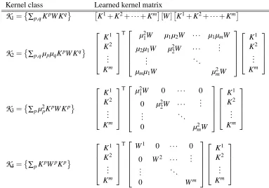
The class of kernels over which Algorithm 4 optimizes can be expressed simply as the set

K

₄=

( _m

∑

p=1

(15)

Kernel class Learned kernel matrix

K

₁=∑_p_,_qKpW Kq K1+K2+_···+Km[W]K1+K2+_···+Km

K

2=∑p,qµpµqKpW Kq

     K1 K2 .. . Km      T     

µ2₁W µ1µ2W _··· µ1µmW

µ2µ1W µ2₂W _··· ... ..

. . ..

µmµ1W µ2mW

           K1 K2 .. . Km     

K

₃=∑_pµ2_pKpW Kp

     K1 K2 .. . Km      T      µ2

1W 0 ··· 0

0 µ2₂W _··· ... ..

. . ..

0 µ2_mW

           K1 K2 .. . Km     

K

₄=∑pKpWpKp

     K1 K2 .. . Km      T     

W1 0 _··· 0

0 W2 ··· ...

..

. . ..

0 Wm

           K1 K2 .. . Km     

Table 1: Block-matrix formulations of metric learning for multiple-kernel formulations (

K

₁–

K

₄). Each Wpis taken to be positive semi-definite. Note that all sets are equal when there is only one base kernel.

Note that

K

₄contains

K

₃ as a special case when all Wpare positive scalar multiples of each-other. However,

K

4leads to a convex optimization problem, where

K

3does not.

Table 1 lists the block-matrix formulations of each of the kernel combination rules described in this section. It is worth noting that it is certainly valid to first form the unweighted combination ker-nelK and then useb

K

₁(Algorithm 3) to learn an optimal projection of the product space. However, as we will demonstrate in Section 5, our proposed multiple-kernel formulation (K₄) outperforms the simple unweighted combination rule in practice.

4.4 Diagonal Learning

The MKPOE optimization is formulated as a semi-definite program over m different n_×n matrices Wp—or, as shown in Table 1, a single mn_×mn PSD matrix with a block-diagonal sparsity structure.

Scaling this approach to large data sets can become problematic, as they require optimizing over multiple high-dimensional PSD matrices.

To cope with larger problems, the optimization problem can be refined to constrain each Wp to the set of diagonal matrices. If Wp are all diagonal, positive semi-definiteness is equivalent to non-negativity of the diagonal values (since they are also the eigenvalues of the matrix). This allows the constraints Wp_{0 to be replaced by linear constraints W}p

(16)

...

(a) Weighted combination (K2)

...

(b) Concatenated projection (K4)

Figure 3: Two variants of multiple-kernel embedding. (a) A data point x_∈

X

is mapped into m fea-ture spaces viaφ1,φ2_{, . . . ,}_φm_{, which are then scaled by µ}_{1,µ2, . . . ,}_µ

mto form a weighted feature space

H

∗_{, which is subsequently projected to the embedding space via M. (b) x is}

first mapped into each kernel’s feature space and then its image in each space is directly projected into a Euclidean space via the corresponding projections Mp. The projections are jointly optimized to produce the embedding space.

Algorithm 4 Multiple kernel partial order embedding (MKPOE) Input: n objects

X

,

partial order

C

,

m kernel matrices K1,K2, . . . ,Km,

β>0

X

_→_Rmn

min Wp_,ξ

m

∑

p=1

tr(WpKp) + β

|

C

_|

∑

_C ξi jkℓ

d(xi,xj)=. m

∑

p=1

K_ip−Kp_j

T

Wp

K_ip−Kp_j

ξi jkℓ≥0 ∀(i,j,k, ℓ)∈

C

Wp0 p=1,2, . . . ,m

More specifically, our implementation of Algorithm 4 operates by alternating sub-gradient de-scent on Wp and projection onto the feasible set Wp0 (see Appendix B for details). For full matrices, this projection is accomplished by computing the spectral decomposition of each Wp, and thresholding the eigenvalues at 0. For diagonal matrices, this projection is accomplished simply by

W_iip_7→max0,W_iip ,

which can be computed in O(mn)time, compared to the O(mn3)time required to compute m spectral decompositions.

(17)

Sneaker Hat White shoe

X-mas teddy Pink animal Ball Big smurf

Lemon Pear Orange

Clothing

Toys

Fruit

All

Figure 4: The label taxonomy for the experiment in Section 5.1.

features encoded in Kp. Note that each of the formulations listed in Table 1 has a corresponding diagonal variant, however, as in the full matrix case, only

K

₁ and

K

₄ lead to convex optimization problems.

5. Experiments

To evaluate our framework for learning multi-modal similarity, we first test the multiple kernel learning formulation on a simple toy taxonomy data set, and then on a real-world data set of musical perceptual similarity measurements.

5.1 Toy Experiment: Taxonomy Embedding

For our first experiment, we generated a toy data set from the Amsterdam Library of Object Images (ALOI) data set (Geusebroek et al., 2005). ALOI consists of RGB images of 1000 classes of objects against a black background. Each class corresponds to a single object, and examples are provided of the object under varying degrees of out-of-plane rotation.

In our experiment, we first selected 10 object classes, and from each class, sampled 20 examples. We then constructed an artificial taxonomy over the label set, as depicted in Figure 4. Using the taxonomy, we synthesized relative comparisons to span subtrees via their least common ancestor. For example,

(Lemon #1,Lemon #2,Lemon #1,Pear#1), (Lemon #1,Pear#,1,Lemon #1,Sneaker#1),

and so on. These comparisons are consistent and therefore can be represented as a directed acyclic graph. They are generated so as to avoid redundant, transitive edges in the graph.

For features, we generated five kernel matrices. The first is a simple linear kernel over the grayscale intensity values of the images, which, roughly speaking, compares objects by shape. The other four are Gaussian kernels over histograms in the (background-subtracted) red, green, blue, and intensity channels, and these kernels compare objects based on their color or intensity distributions. We augment this set of kernels with five “noise” kernels, each of which was generated by sam-pling random points from the unit sphere inR3_{and applying the linear kernel.}

(18)

each fold, we learned a diagonally-constrained embedding with Algorithm 4, using the subset of relative comparisons (i,j,k, ℓ) with i,j,k and ℓ restricted to the training set. After learning the embedding, the held out data (validation or test) was mapped into the space, and the accuracy of the embedding was determined by counting the fraction of correctly predicted relative comparisons. In the validation and test sets, comparisons were processed to only include comparisons of the form

(i,j,i,k)where i belongs to the validation (or test) set, and j and k belong to the training set. We repeat this experiment for each base kernel individually (that is, optimizing over

K

₁ with a single base kernel), as well as the unweighted sum kernel (

K

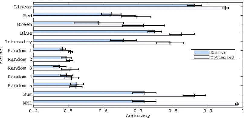
₁with all base kernels), and finally MKPOE (K4 with all base kernels). The results are averaged over all training/test splits, and

col-lected in Figure 5. For comparison purposes, we include the prediction accuracy achieved by com-puting distances in each kernel’s native space before learning. In each case, the optimized space indeed achieves higher accuracy than the corresponding native space. (Of course, the random noise kernels still predict randomly after optimization.)

As illustrated in Figure 5, taking the unweighted combination of kernels significantly degrades performance (relative to the best kernel) both in the native space (0.718 accuracy versus 0.862 for the linear kernel) and the optimized sum-kernel space (0.861 accuracy for the sum versus 0.951 for the linear kernel), that is, the unweighted sum kernel optimized by Algorithm 3. However, MKPOE (

K

₄) correctly identifies and omits the random noise kernels by assigning them negligible weight, and achieves higher accuracy (0.984) than any of the single kernels (0.951 for the linear kernel, after learning).

5.2 Musical Artist Similarity

To test our framework on a real data set, we applied the MKPOE algorithm to the task of learning a similarity function between musical artists. The artist similarity problem is motivated by several real-world applications, including recommendation and playlist-generation for online radio. Be-cause artists may be represented by a wide variety of different features (e.g., tags, acoustic features, social data), such applications can benefit greatly from an optimally integrated similarity metric.

The training data is derived from the aset400 corpus of Ellis et al. (2002), which consists of 412 popular musicians, and 16385 relative comparisons of the form(i,j,i,k). Relative comparisons were acquired from human test subjects through a web survey; subjects were presented with a query artist (i), and asked to choose what they believe to be the most similar artist ( j) from a list of 10 candidates. From each single response, 9 relative comparisons are synthesized, indicating that j is more similar to i than the remaining 9 artists (k) which were not chosen.

Our experiments here replicate and extend previous work on this data set (McFee and Lanck-riet, 2009a). In the remainder of this section, we will first give an overview of the various types of features used to characterize each artist in Section 5.2.1. We will then discuss the experimental pro-cedure in more detail in Section 5.2.2. The MKL embedding results are presented in Section 5.2.3, and are followed by an experiment detailing the efficacy of our constraint graph processing approach in Section 5.2.4.

5.2.1 FEATURES

(19)

Linear

Red

Green

Blue

Intensity

Random 1

Random 2

Random 3

Random 4

Random 5

Sum

MKL

0.4 0.5 0.6 0.7 0.8 0.9 1

Kernel

Accuracy

Native Optimized

Figure 5: Mean test set accuracy for the experiment of Section 5.1. Error bars correspond to one standard deviation across folds. Accuracy is computed by counting the fraction of cor-rectly predicted relative comparisons in the native space of each base kernel, and then in the optimized space produced by KPOE (

K

₁with a single base kernel). The unweighted combination of kernels (Sum) significantly degrades performance in both the native and optimized spaces. MKPOE (MKL,

K

₄) correctly rejects the random kernels, and signifi-cantly outperforms the unweighted combination and the single best kernel.

• MFCC: for each artist, we collected between 1 and 10 songs (mean 4). For each song,

we extracted a short clip consisting of 10000 half-overlapping 23ms windows. For each window, we computed the first 13 Mel Frequency Cepstral Coefficients (MFCCs) (Davis and Mermelstein, 1990), as well as their first and second instantaneous derivatives. This results in a sequence of 39-dimensional vectors (delta-MFCCs) for each song. Each artist i was then summarized by a Gaussian mixture model (GMM) pi over delta-MFCCs extracted from the corresponding songs. Each GMM has 8 components and diagonal covariance matrices. Finally, the kernel between artists i and j is the probability product kernel (Jebara et al., 2004) between their corresponding delta-MFCC distributions pi,pj:

K_{i j}mfcc=

Z q

pi(x)pj(x)dx.

• Auto-tags (AT): Using the MFCC features described above, we applied the automatic tagging

algorithm of Turnbull et al. (2008), which for each song yields a multinomial distribution over a set T of 149 musically-relevant tag words (auto-tags). Artist-level tag distributions qiwere formed by averaging model parameters (i.e., tag probabilities) across all of the songs of artist

(20)

χ2_{-distance between the multinomial distributions q}

i and qj:

K_{i j}at=exp ₋σ

∑

t∈T

(qi(t)−qj(t))2

qi(t) +qj(t)

!

.

In these experiments, we fixedσ=256.

• Social tags (ST): For each artist, we collected the top 100 most frequently used tag words

from Last.fm,2 a social music website which allows users to label songs or artists with ar-bitrary tag words or social tags. After stemming and stop-word removal, this results in a vocabulary of 7737 tag words. Each artist is then represented by a bag-of-words vector in

R7737, and processed by TF-IDF. The kernel between artists for social tags is the cosine sim-ilarity (linear kernel) between TF-IDF vectors.

• Biography (Bio): Last.fm also provides textual descriptions of artists in the form of

user-contributed biographies. We collected biographies for each artist in the aset400 data set, and after stemming and stop-word removal, we arrived at a vocabulary of 16753 biography words. As with social tags, the kernel between artists is the cosine similarity between TF-IDF bag-of-words vectors.

• Collaborative filtering (CF): Celma (2008) collected collaborative filtering data from Last.fm

in the form of a bipartite graph over users and artists, where each user is associated with the artists in her listening history. We filtered this data down to include only the aset400 artists, of which all but 5 were found in the collaborative filtering graph. The resulting graph has 336527 users and 407 artists, and is equivalently represented by a binary matrix where each row i corresponds to an artist, and each column j corresponds to a user. The i j entry of this matrix is 1 if we observe a user-artist association, and 0 otherwise. The kernel between artists in this view is the cosine of the angle between corresponding rows in the matrix, which can be interpreted as counting the amount of overlap between the sets of users listening to each artist and normalizing for overall artist popularity. For the 5 artists not found in the graph, we fill in the corresponding rows and columns of the kernel matrix with the identity matrix.

5.2.2 EXPERIMENTALPROCEDURE

The data was randomly partitioned into ten 90/10 training/test splits. Given the inherent ambiguity in the task, and format of the survey, there is a great deal of conflicting information in the survey responses. To obtain a more accurate and internally consistent set of training comparisons, directly contradictory comparisons (e.g.,(i,j,i,k)and(i,k,i,j)) were removed from both the training and test sets. Each training set was further cleaned by finding an acyclic subset of comparisons and taking its transitive reduction, resulting in a minimal partial order. (No further processing was performed on test comparisons.)

After training, test artists were mapped into the learned space (by Equation 9), and accuracy was measured by counting the number of measurements(i,j,i,k)correctly predicted by distance in the learned space, where i belongs to the test set, and j,k belong to the training set.

For each experiment,βis chosen from_{10−2,10−1, . . . ,107_}by holding out 30% of the training constraints for validation. (Validation splits are generated from the unprocessed training set, and the

(21)

MFCC

Auto−tags

Social tags

Biography

Collab. Filter

0 0.1 0.2 0.3 0.4 0.5 0.6 0.7 0.8 0.9 1

Accuracy

Native Diagonal Full

Figure 6: aset400 embedding results for each of the base kernels. Accuracy is computed in each kernel’s native feature space, as well as the space produced by applying Algorithm 3 (i.e., optimizing over

K

₁ with a single kernel) with either the diagonal or full-matrix formulation. Error bars correspond to one standard deviation across training/test splits.

remaining training constraints are processed as described above.) After finding the best-performing

β, the embedding is trained on the full (processed) training set.

5.2.3 EMBEDDINGRESULTS

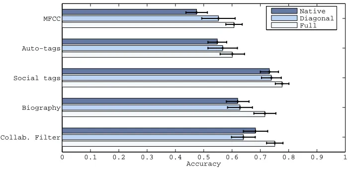
For each base kernel, we evaluate the test-set performance in the native space (i.e., by distances calculated directly from the entries of the kernel matrix), and by learned metrics, both diagonal and full (optimizing over

K

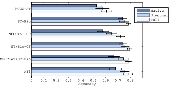
₁with a single base kernel). Figure 6 illustrates the results.

We then repeated the experiment by examining different groupings of base kernels: acoustic (MFCC and Auto-tags), semantic (Social tags and Bio), social (Collaborative filter), and combina-tions of the groups. The different sets of kernels were combined by Algorithm 4 (optimizing over

K

4). The results are listed in Figure 7.

In all cases, MKPOE improves over the unweighted combination of base kernels. Moreover, many combinations outperform the single best kernel (ST, 0.777±0.02 after optimization), and the algorithm is generally robust in the presence of poorly-performing kernels (MFCC and AT). Note that the poor performance of MFCC and AT kernels may be expected, as they derive from song-level rather than artist-level features, whereas ST provides high-level semantic descriptions which are generally more homogeneous across the songs of an artist, and Bio and CF are directly constructed at the artist level. For comparison purposes, we trained metrics on the sum kernel with

K

₁ (Algorithm 3), resulting in accuracies of 0.676_±0.05 (diagonal) and 0.765_±0.03 (full). The proposed approach (Algorithm 4) applied to all kernels results in 0.754_±0.03 (diagonal), and 0.795_±0.02 (full).

(22)

MFCC+AT

ST+Bio

MFCC+AT+CF

ST+Bio+CF

MFCC+AT+ST+Bio

All

0 0.1 0.2 0.3 0.4 0.5 0.6 0.7 0.8

Accuracy

Native Diagonal Full

Figure 7: aset400 embedding results with multiple kernel learning: the learned metrics are opti-mized over

K

₄by Algorithm 4. Native corresponds to distances calculated according to the unweighted sum of base kernels.

by the algorithm, and the majority of the weight is assigned to the (highest-performing) social tag (ST) kernel.

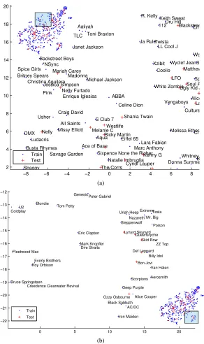
A t-SNE (van der Maaten and Hinton, 2008) visualization of the space produced by MKPOE is illustrated in Figure 9. The embedding captures a great deal of high-level genre structure: for example, the classic rock and metal genres lie at the opposite end of the space from pop and

hip-hop.

5.2.4 GRAPHPROCESSINGRESULTS

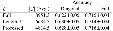
To evaluate the effects of processing the constraint set for consistency and redundancy, we repeat the experiment of the previous section with different levels of processing applied to

C. Here, we

focus on the Biography kernel, since it exhibits the largest gap in performance between the native and learned spaces.

As a baseline, we first consider the full set of similarity measurements as provided by human judgements, including all inconsistencies. To first deal with what appear to be the most egregious inconsistencies, we prune all directly inconsistent training measurements; that is, whenever(i,j,i,k)

and (i,k,i,j) both appear, both are removed.3 Finally, we consider the fully processed case by finding a maximal consistent subset (partial order) of

C

and removing all redundancies. Table 2 lists the number of training constraints retained by each step of processing (averaged over the random splits).

Using each of these variants of the training set, we test the embedding algorithm with both diagonal and full-matrix formulations. The results are presented in Table 2. Each level of graph processing results in a significant reduction in the number of training comparisons (and, therefore,

(23)

0 0.5 1

MFCC

0 0.5

AT

0 0.5

ST

0 0.5

Bio

0 50 100 150 200 250 300

0 0.5

CF

Figure 8: The weighting learned by Algorithm 4 using all five kernels and diagonal Wp. Each bar plot contains the diagonal of the corresponding kernel’s learned metric. The horizontal axis corresponds to the index in the training set, and the vertical axis corresponds to the learned weight in each kernel space.

Accuracy

C

_|

C

_|(Avg.) Diagonal Full

Full 8951.3 0.622_±0.05 0.715_±0.04

Length-2 6684.5 0.630_±0.05 0.714_±0.04

Processed 4814.5 0.628_±0.05 0.716_±0.04

Table 2: aset400 embedding results (Biography kernel) for three possible refinements of the con-straint set. Full includes all similarity measurements, with no pruning for consistency or redundancy. Length-2 removes all length-2 cycles (i.e.,(i,j,k, ℓ)and(k, ℓ,i,j)). Processed finds an approximate maximal consistent subset, and removes redundant constraints.

computational overhead of Algorithm 3), while not degrading the quality of the resulting embed-ding.

(24)

−8 −6 −4 −2 0 2 4 6 8 2 4 6 8 10 12 14 16 18 20 Lara Fabian Bette Sixpence None the Richer

Michael Jackson Suga Spice Girls Twista Eiffel 65 R. Kelly ABBA Usher Keith Sweat *NSync Dru Hill Janet Jackson Xzibit Melissa Etheridg Shaggy

LL Cool J

Craig David Culture Be

Britney Spears Spin Pink Jessica Simpson Vengaboys DMX Wyclef Jean White Zombie Enrique Iglesias 112 Coolio Alice D Missy Elliott Natalie Imbruglia All Saints Aaliyah Toni Braxton Marc Anthony Christina Aguilera Donna Summer Ludacris En Vo Backstreet Boys Aqua Celine Dion Busta Rhymes Whitney Ho Chic S Club 7

War TLC Savage Garden Ja Rule Ric Madonna

Ace of Base

Blackstreet LFO Ricky Martin The Corrs Melanie C Kenny G Nelly Matthew S Nelly Furtado La B Shania Twain Mariah Carey Cyndi Lauper

Ugly Kid Joe

Westlife Soul Asy Red Train Test (a)

0 5 10 15 20

−22 −21 −20 −19 −18 −17 −16 −15 −14 −13 −12 Mark Knopfler

Dire Straits ZZ Top

U2 Steppenwolf Bruce Springsteen Tom Petty Peter Gabriel Mr. Big Roy Orbison Everly Brothers Tesla Black Sabbath Eric Clapton Coldplay Aerosmith Fleetwood Mac Billy Idol Deep Purple Alice Cooper Nazareth

Creedence Clearwater Revival

Scorpions

Iron Maiden AC/DC

Poison Uriah HeepExtreme Blondie Van Halen Genesis Lynyrd Skynyrd Skid Row Queensryche Bon Jovi Ozzy Osbourne Def Leppard Train Test (b)

(25)

1 2 3 4 5 6 7 8 9 10

0 0.1 0.2 0.3 0.4 0.5 0.6 0.7 0.8 0.9 1

Split #

Accuracy

Figure 10: Accuracy of the learned embedding for each training/test split, averaged over ten tri-als with random maximal acyclic constraint subgraphs. Error bars correspond to one standard deviation.

6. Hardness of Dimensionality Reduction

The algorithms given in Sections 3 and 4 attempt to produce low-dimensional solutions by regular-izing W , which can be seen as a convex approximation to the rank of the embedding. In general, because rank constraints are not convex, convex optimization techniques cannot efficiently mini-mize dimensionality. This does not necessarily imply other techniques could not work. So, it is natural to ask if exact solutions of minimal dimensionality can be found efficiently, particularly in the multidimensional scaling scenario, that is, when K=I (Section 3.3).

As a special case, one may wonder if any instance(

X

,

C

)can be satisfied inR1. As Figure 11 demonstrates, not all instances can be realized in one dimension. Even more, we show that it is NP-Complete to decide if a given

C

can be satisfied inR1. Given an embedding, it can be verified in polynomial time whether

C

is satisfied or not by simply computing the distances between all pairs and checking each comparison in

C

, so the decision problem is in NP. It remains to show that the

R1partial order embedding problem (hereafter referred to as 1-POE) is NP-Hard. We reduce from the Betweenness problem (Opatrny, 1979), which is known to be NP-complete.

Definition 1 (Betweenness) Given a finite set Z and a collection T of ordered triples (a,b,c) of distinct elements from Z, is there a one-to-one function f : Z→Rsuch that for each(a,b,c)_∈ T , either f(a)< f(b)< f(c)or f(c)< f(b)< f(a)?

Theorem 1 1-POE is NP-Hard.

Proof Let (Z,T) be an instance of Betweenness. Let

X

=Z, and for each (a,b,c)_∈ T ,

intro-duce constraints(a,b,a,c)and(b,c,a,c)to

C

. Since Euclidean distance inR1 is simply line dis-tance, these constraints force g(b)to lie between g(a) and g(c). Therefore, the original instance

(Z,T)_∈Betweenness if and only if the new instance(

X

,

C

)_∈1-POE. Since Betweenness is NP-Hard, 1-POE is NP-Hard as well.

(26)

A

B

C

D

(a)

AD

BC

CD AC BD

AB

(b)

Figure 11: (a) The vertices of a square inR2_{. (b) The partial order over distances induced by the}

square: each side is less than each diagonal. This constraint set cannot be satisfied in

R1.

7. Conclusion

We have demonstrated a novel method for optimally integrating heterogeneous data to conform to measurements of perceptual similarity. By interpreting a collection of relative similarity compar-isons as a directed graph over pairs, we are able to apply graph-theoretic techniques to isolate and prune inconsistencies in the training set and reduce computational overhead by eliminating redun-dant constraints in the optimization procedure.

Our multiple-kernel formulation offers a principled way to integrate multiple feature modalities into a unified similarity space. Our formulation carries the intuitive geometric interpretation of con-catenated projections, and results in a semidefinite program. By incorporating diagonal constraints as well, we are able to reduce the computational complexity of the algorithm, and learn a model which is both flexible—only using kernels in the portions of the space where they are informative— and interpretable—each diagonal weight corresponds to the contribution to the optimized space due to a single point within a single feature space. Table 1 provides a unified perspective of multiple kernel learning formulations for embedding problems, but it is clearly not complete. It will be the subject of future work to explore and compare alternative generalizations and restrictions of the formulations presented here.

Acknowledgments

The authors acknowledge support from NSF Grant DMS-MSPA 0625409 and eHarmony, Inc.

Appendix A. Embedding Partial Orders

In this appendix, we prove that any set

X

with a partial order over distances

C

can be embedded intoRnwhile satisfying all distance comparisons.

(27)

Algorithm 5 Naïve total order construction Input: objects

X

, partial order

C

Output: symmetric dissimilarity matrix∆_∈Rn×n

for each i in 1. . .n do ∆ii←0

end for

for each(k, ℓ)in topological order do

if in-degree(k, ℓ) =0 then

∆kℓ,∆ℓk←1

else

∆kℓ,∆ℓk← max

(i,j,k,ℓ)∈C∆i j+1 end if

end for

general,

C

is not a total order, but a

C

-respecting embedding can always be produced by reducing the partial order to a (weak) total order by topologically sorting the graph (see Algorithm 5).

Let∆be the dissimilarity matrix produced by Algorithm 5 on an instance(