A NUMERICAL STUDY OF FLOW AND HEAT TRANSFER
BETWEEN TWO ROTATING VERTICALLY ECCENTRIC
SPHERES WITH TIME- DEPENDENT
ANGULAR VELOCITIES
A. Jabari Moghadam and A. Baradaran Rahimi*
Faculty of Engineering, Ferdowsi University of Mashhad P.O. Box 91775-1111, Mashhad, Iran
*Corresponding Author
(Received: March 2, 2007 – Accepted in Revised Form: May 9, 2008)
Abstract The transient motion and the heat transfer of a viscous incompressible flow contained between two vertically eccentric spheres maintained at different temperatures and rotating about a common axis with different angular velocities is numerically considered when the angular velocities are an arbitrary functions of time. The resulting flow pattern, temperature distribution, and heat transfer characteristics are presented for the various cases including exponential and sinusoidal angular velocities. Interesting effect of long delays in heat transfer of large portions of the fluid in the annulus is observed because of the angular velocities of the corresponding spheres. As the eccentricity increases and the gap between the spheres decreases, the coriolis forces and convection heat transfer effect in the narrower portion increase.
Keywords Flow And Heat Transfer, Vertically Eccentric Rotating Spheres, Time-Dependent Angular Velocities, Numerical Solution
ﻩﺪﻴﻜﭼ
ﯼﺎﻣﺮﮔ ﻝﺎﻘﺘﻧﺍﻭﻥﺎﻳﺮﺟﯼﺎﻫﺎﻣﺩﺭﺩﻪﮐﺰﮐﺮﻣﺯﺍﺝﺭﺎﺧﻩﺮﮐﻭﺩﻦﻴﺑﺮﻳﺬﭘﺎﻧ ﻢﮐﺍﺮﺗﺝﺰﻟﻝﺎﻴﺳﮏﻳﯼﺍﺭﺬﮔ
ﯽﻣﺕﻭﺎﻔﺘﻣﯼﺍ ﻪﻳﻭﺍﺯﯼﺎﻫ ﺖﻋﺮﺳﺎﺑﮎﺮﺘﺸﻣﺭﻮﺤﻣﮏﻳﻝﻮﺣ ﺭﺩﺶﺧﺮﭼﻝﺎﺣﺭﺩﻭﻩﺩﻮﺑ ﺕﻭﺎﻔﺘﻣ ﻪﺑﺍﺭﺪﻨﺷﺎﺑ
ﯽﻣﺭﺍﺮﻗﻪﻌﻟﺎﻄﻣﺩﺭﻮﻣﯼﺩﺪﻋﺕﺭﻮﺻ ﻢﻴﻫﺩ
. ﻣﻥﺎﻣﺯﻊﺑﺎﺗﯼﺍﻪﻳﻭﺍﺯﯼﺎﻫﺖﻋﺮﺳ ﯽ
ﺪﻨﺷﺎﺑ . ﺎﻣﺩﻊﻳﺯﻮﺗﻭﻥﺎﻳﺮﺟﯼﻮﮕﻟﺍ
ﻪﻳﺍﺭﺍ ﯽﺳﻮﻨﻴﺳﻭﯽﻳﺎﻤﻧﯼﺍ ﻪﻳﻭﺍﺯﯼﺎﻫﺖﻋﺮﺳﻞﻴﺒﻗﺯﺍﯽﺗﻭﺎﻔﺘﻣﯼﺎﻫﺖﻴﻌﺿﻭ ﯼﺍﺮﺑﺎﻣﺮﮔﻝﺎﻘﺘﻧﺍﯼﺎﻫﻪﺼﺨﺸﻣﻭ ﺪﻧﺍ ﻩﺪﺷ . ﯼﺍ ﻪﻳﻭﺍﺯ ﯼﺎﻫ ﺖﻋﺮﺳ ﻦﻳﺍ ﺮﻃﺎﺧ ﻪﺑ ﻩﺮﮐ ﻭﺩ ﻦﻴﺑ ﻪﻴﺣﺎﻧ ﺯﺍ ﯽﮔﺭﺰﺑ ﺖﻤﺴﻗ ﺭﺩ ﺎﻣﺮﮔ ﻝﺎﻘﺘﻧﺍﺭﺩ ﺮﻴﺧﺎﺗ
ﯽﻣﻩﺪﻫﺎﺸﻣ ﺩﻮﺷ
. ﺎﺧﺶﻳﺍﺰﻓﺍﻦﻤﺿﻦﻴﻨﭽﻤﻫ ﻪﺑﺏﺬﺟﯼﺎﻫﻭﺮﻴﻧﻩﺮﮐﻭﺩﻦﻴﺑﻪﻠﺻﺎﻓﺶﻫﺎﮐﻭﻩﺮﮐﻭﺩﯼﺰﮐﺮﻣﺯﺍﺝﺭ
ﯽﻣﺶﻳﺍﺰﻓﺍﺮﺘﮑﻳﺭﺎﺑﺖﻤﺴﻗﺭﺩﯽﻳﺎﺠﺑﺎﺟﯼﺎﻣﺮﮔﻝﺎﻘﺘﻧﺍﺮﺛﺍﻭﺰﮐﺮﻣ ﺪﺑﺎﻳ
.
1. INTRODUCTION
The transient motion of an incompressible viscous flow and its heat transfer in a rotating spherical annuli is considered numerically when the spheres are vertically eccentric and their angular velocities about a common axis of rotation may be arbitrarily-prescribed as functions of time. Such motions may be described in terms of a pair of coupled non-linear partial differential equations in three independent variables and the energy equation is linear when velocity field is known. Available theoretical work concerning such problems is primarily of a boundary-layer or
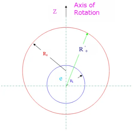
Figure 1. Geometry of eccentric rotating spheres. Reynolds numbers. Thermal convection in rotating
spherical annuli has been considered by Douglass, et al [10] in which the steady forced convection of a viscous fluid contained between two concentric spheres which are maintained at different temperatures and rotate about a common axis with different angular velocities is studied. Approximate solutions to the governing equations are obtained in terms of a regular perturbation solution valid for small Reynolds number and a modified Galerkian solution for moderate Reynolds numbers. Viscous dissipation is neglected in their study and all fluid properties are assumed constant. A study of viscous flow in oscillatory spherical annuli has been done by Munson, et al [11] in which a perturbation solution valid for slow oscillation rates is presented and compared with experimental results. Another interesting work is the study of the axially symmetric motion of an incompressible viscous fluid between two concentric rotating spheres done by Gagliardi, et al [12]. This work involves study of the steady state and transient motion of a system consisting of an incompressible, Newtonian fluid in an annulus between two concentric, rotating, rigid spheres. The primary purpose of their research is to study the use of an approximate analytical method for analyzing the transient motion of the fluid in the annulus and spheres which started suddenly due to the action of prescribed torques and also the study by Yang, et al [13] and the finite element study by Ni, et al [14]. These problems include the case where one or both spheres rotate with prescribed constant angular velocities and the case in which one sphere rotates due to the action of an applied constant or impulsive torque. The most recent undertakings regarding spherical annuli are similarity solution in the study of flow and heat transfer between two rotating spheres with constant angular velocities by Jabari Moghadam, et al [15] and numerical study of flow and heat transfer between two rotating spheres by Jabari Moghadam, et al [16] which considers the time-dependency of the angular velocities.
The study of transient motion and heat transfer of an incompressible viscous fluid filling the annuli of two vertically eccentric spheres rotating with any prescribed function of time angular velocity has not been considered in the literature. In the present study a numerical solution of
unsteady momentum and energy equations is presented for viscous flow between two vertically eccentric rotating spheres maintained at different temperatures which are rotating with time-dependent angular velocities. Results for some time-dependent rotation functions including exponential and sinusoidal angular velocities are presented when the outer sphere initially starts rotating with a constant angular velocity and the inner sphere starts rotating with a prescribed time-dependent function. Such a rotating containers are used in engineering designs like centrifuges and fluid gyroscopes and also are important in geophysics.
2. PROBLEM FORMULATION
is a function of θ. A Newtonian, viscous, incompressible fluid fills the gap between the inner and outer spheres which are of radii Ri and Ro and with constant surface temperatures Ti and To and rotate about a common axis with angular velocities Ωi a n d Ωo, res p ectively . The components of velocity in directions r, θ, and φ are vr, vθ, and vφ, respectively. These velocity components for incompressible flow and in meridian plane satisfy the continuity equation and are related to stream function ψ and angular momentum function Ω in the following manner:
θ θ ψ = sin 2 r r v , θ ψ − = θ sin r r v , θ Ω = φ sin r
v (1)
Since the flow is assumed to be independent of the longitude, φ, the non-dimensional Navier-Stokes equations and energy equation can be written in terms of the stream function and the angular velocity function as follows:
Ω = θ θ Ω ψ − Ω θ ψ + ∂ Ω ∂ 2 D (Re) 1 sin 2 r r r
t (2)
ψ = θ θ ψ − θ ψ θ ψ + ψ θ ψ − θ ψ ψ θ − θ θ Ω − θ Ω θ Ω + ψ ∂ ∂ 4 D (Re) 1 ] sin cos r r [ 2 sin 3 r 2 D 2 ] r ) 2 D ( ) 2 D ( r [ sin 2 r 1 ] sin cos r r [ 2 sin 3 r 2 ) 2 D ( t (3) } 2 )] r v ( r r [ 2 )] sin v ( r sin [ 2 ] r v r 1 ) r v ( r r [ ] 2 ) cot r v r r v ( 2 ) rr v v r 1 ( 2 ) rr v [( 2 ){ Ek ( ] T 2 r cot 2 T 2 2 r 1 r T r 2 2 r T 2 [ ) Pe ( 1 T r v r T r v t T φ ∂ ∂ + θ φ θ ∂ ∂ θ + θ ∂ ∂ + θ ∂ ∂ + θ θ + + + θ ∂θ ∂ + ∂ ∂ + θ ∂ ∂ θ + θ ∂ ∂ + ∂ ∂ + ∂ ∂ = θ ∂ ∂ θ + ∂ ∂ + ∂ ∂ (4) In which the non-dimensional quantities Reynolds
number (Re), Prandtl number (Pr), Peclet number (Pe), and Eckert number (Ek) are defined as:
ν ω = 2 o r o
Re , Pr=ν/α,
α ω = = 2 o r o Pr . Re Pe , ) i T o T ( P c o Ek − νω
= (5)
The following non-dimensional parameters have been used in the above equations and then the asterisks have been omitted:
o t t∗= ω ,
o r
r r∗= ,
o 3 o r ω ψ = ∗ ψ , o 2 o r ω Ω = ∗ Ω , i T o T i T T T − − =
∗ (6)
In which ro and ωo are reference values. The non-dimensional boundary and initial conditions for the above governing equations are:
For tp0:
⎪ ⎩ ⎪ ⎨ ⎧ = = Ω = ψ 0 T 0 0
, every where
For t≥0:
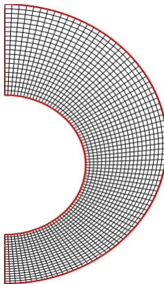
Figure 2. A typical mesh grid. Where,
θ
2 r
θ
cot 2
θ
2 2 r
1 2 r
2 2 D
∂ ∂ − ∂
∂ + ∂
∂
≡ . (8)
These governing equations along with the related boundary and initial conditions are solved numerically in the next section.
3. COMPUTATIONAL PROCEDURE
The two equations governing the fluid motion show that each is describing the behavior of one of the dependent variables Ω and ψ. On the other hand, these two equations are coupled only through nonlinear terms. To solve the problem, the momentum equations were discretized by the finite-difference method and implicit-explicit schemes. Because of the known velocity field, the energy equation is linear and is solved keeping all its terms. In each time step (n + 1), the value of the dependent variables are guessed from their values at previous time steps (n), (n-1), and (n-2) and after using them in difference equations and repeating this, until obtaining the desired convergence, will lead to the corrected values at this time step. This procedure is applied for the next time step.
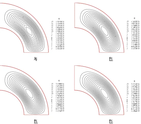
The flow field considered is covered with a regular mesh, see Figure 2. To solve the system of linear difference equations, a tri-diagonal method algorithm is used in both directions r and θ, Press, et al [17]. Direct substitution of previous values of dependent variables by new calculated values can cause calculation un-stability in general. To overcome this problem, a weighting procedure is used in which the optimum weighting factor depends on Reynolds number. The mesh size used in numerical solution for equator of the circle is 40 x 20 or 50 x 25. A mesh independence study has been demonstrated in Figures 3 and 4. In this mesh-study, the conditions of flow and heat transfer fields are: Re = 10, Pr = 10, Ek = 0, and
io
Ω = 0. As it can be seen, the difference between the contours of ψ function for the coarse grid (case (a), with mesh size 25*12) and the fine grid (case (b) with mesh size 40*20) is almost large (about 12 %), but the difference between case (c)
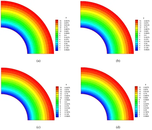
(with grid size 45*25) and case (d) (with grid size 50*25) is really negligible (less than 0.03 %). Hence the numerical solution is mesh-independent for cases c or d and even b. For the results presented in our solution, a 50*25 mesh grid has been selected though a 40*20 mesh would have been fine. The mesh sizes mentioned above are in θ x r directions. The contours of temperature has also been drawn for mesh sizes from case (a), 25*12 to case (d), 50*25 in Figure 4. In this case no significant differences between these cases can be seen and that is because the energy equation is linear and its solution has much less complexities compared with momentum equation.
1
1 2
2
3
3 4
4 5
5 6
6 7
7
8
8
9
1
0
11
12 15
15 4.5095E-04
14 4.2088E-04
13 3.9082E-04
12 3.6075E-04
11 3.3068E-04
10 3.0062E-04
9 2.7055E-04
8 2.4048E-04
7 2.1041E-04
6 1.8035E-04
5 1.5028E-04
4 1.2021E-04
3 9.0147E-05
2 6.0080E-05
1 3.0013E-05
ψ
1
1
2
2
3 3
4
4 5
5
6 7
7 8
9
9
10 11
12 13
15
15 4.9703E-04
14 4.6389E-04
13 4.3076E-04
12 3.9762E-04
11 3.6449E-04
10 3.3135E-04
9 2.9822E-04
8 2.6508E-04
7 2.3195E-04
6 1.9881E-04
5 1.6568E-04
4 1.3254E-04
3 9.9406E-05
2 6.6270E-05
1 3.3135E-05
ψ
(a) (b)
1
1
1 2
2 3
3
4
4 5
5 6 7
7 8
8
9
10 11
12
13
15 5.1266E-04
14 4.7848E-04
13 4.4430E-04
12 4.1012E-04
11 3.7593E-04
10 3.4175E-04
9 3.0757E-04
8 2.7339E-04
7 2.3921E-04
6 2.0503E-04
5 1.7084E-04
4 1.3666E-04
3 1.0248E-04
2 6.8299E-05
1 3.4117E-05
ψ
1
1
2
2 2
3
3 45
6 7
7 8
8 9
10 1211
15
15 5.1254E-04
14 4.7837E-04
13 4.4419E-04
12 4.1001E-04
11 3.7584E-04
10 3.4166E-04
9 3.0748E-04
8 2.7331E-04
7 2.3913E-04
6 2.0495E-04
5 1.7077E-04
4 1.3660E-04
3 1.0242E-04
2 6.8244E-05
1 3.4067E-05
ψ
(c) (d)
Figure 3. Contours of stream function for various mesh-size grid.
4. PRESENTATION OF RESULTS
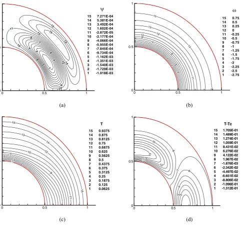
If the bounding spherical surfaces were stationary, there would be no fluid motion and the temperature distribution would simply be conduction distribution. Any rotation of the bounding spheres sets up a primary flow (ω) around the axis of rotation. This relative motion induces an unbalanced centrifugal force field which drives the secondary flows (ψ) in the meridian plane. Thus, if the bounding spheres are of unequal temperatures, this secondary flow produces forced convection within the annulus, resulting in a temperature
distribution which is different from the pure conduction distribution. The relative magnitudes of the secondary flow and forced convection effects depend upon the parameters involved, including those concerning the geometry and dynamics of the flow such as Ωio = Ωi/Ωo, Rio = Ri/Ro,
15 0.9375
14 0.875
13 0.8125
12 0.75
11 0.6875
10 0.625
9 0.5625
8 0.5
7 0.4375
6 0.375
5 0.3125
4 0.25
3 0.1875
2 0.125
1 0.0625
T
15 0.9375
14 0.875
13 0.8125
12 0.75
11 0.6875
10 0.625
9 0.5625
8 0.5
7 0.4375
6 0.375
5 0.3125
4 0.25
3 0.1875
2 0.125
1 0.0625
T
(a) (b)
15 0.9375
14 0.875
13 0.8125
12 0.75
11 0.6875
10 0.625
9 0.5625
8 0.5
7 0.4375
6 0.375
5 0.3125
4 0.25
3 0.1875
2 0.125
1 0.0625
T
15 0.9375
14 0.875
13 0.8125
12 0.75
11 0.6875
10 0.625
9 0.5625
8 0.5
7 0.4375
6 0.375
5 0.3125
4 0.25
3 0.1875
2 0.125
1 0.0625
T
(c) (d)
Figure 4. Contours of stream function for various mesh-size grid.
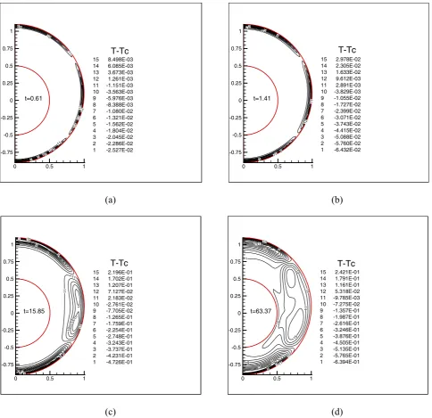
of the effect of secondary flows on temperature distribution, the contours of (T-Tc) are also
presented in this study which show the difference between actual temperature and the pure conduction case. Here, Tc depends only on r. The
flow and temperature fields are symmetric with respect to the rotation axis and also the equator plane if the spheres are concentric. But when the spheres are eccentric then the flow and temperature fields are only symmetric with respect to the axis of rotation. The cases considered here include time-dependent angular velocities which are
exponential and sinusoidal. Results for velocity and temperature fields are presented for cases when the outer sphere is rotating with a constant angular velocity and the inner sphere starts rotating with the prescribed function of time angular velocities. These presentations are only at some selected time values.
The velocity fields for the particular case of inner sphere angular velocity, Ωio = -exp (1-t), and
TABLE 1. Results of References [8-10] for Re = 50, Ωio = -3, and Pr = 10.
T
ω
104ψ
Contour Number
0.06 -2.76
-19 1
0.12 -2.6
-17 2
0.18 -2.2
-15 3
0.26 -2
-13.5 4
0.3 -1.78
-11.5 5
0.38 -1.55
-10 6
0.44 -1.2
-7.8 7
0.51 -1.05
-6 8
0.57 -0.77
-4 9
0.63 -0.52
-2.1 10
0.68 -0.22
-2.8 11
0.76 0.01
1.6 12
0.82 0.26
3.5 13
0.88 0.52
5.4 14
0.94 0.77
7.3 15
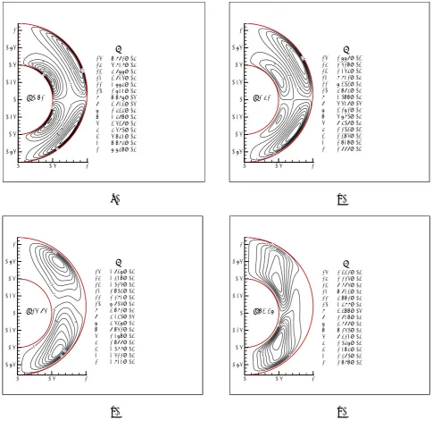
values. At the beginning when the vortices (ψ
contours) are formed, it is seen that the annulus space is under the effect of both spheres which are dominating the flow field.
A clockwise vortex close to outer sphere and a counterclockwise vortex close to the inner sphere (both in first quadrant) are formed, Figure 6a,b. The size and the direction of these vortices are different in fourth quadrant because of the eccentricity. This factor also causes the vortices in first quadrant to penetrate into the fourth quadrant and compress the vortices in this region. As the inner angular velocity decreases with time, its effect on the secondary flow diminishes. During this time the clockwise vortex grows considerably and after some time there is only one big
0 0.5 1 0
5
1 3
4 5
6
7
7 8
8
9
10
10 11
11
12
12 13
13
14
15
15 7.271E-04
14 5.381E-04
13 3.492E-04
12 1.602E-04
11 -2.872E-05
10 -2.177E-04
9 -4.066E-04
8 -5.955E-04
7 -7.845E-04
6 -9.734E-04
5 -1.162E-03
4 -1.351E-03
3 -1.540E-03
2 -1.729E-03
1 -1.918E-03
ψ
00 0.5 1
0.5 1
2 3
4 5
6 7
8
9 10
11
12 13
14
15
15
15 0.75
14 0.5
13 0.25
12 0
11 -0.25
10 -0.5
9 -0.75
8 -1
7 -1.25
6 -1.5
5 -1.75
4 -2
3 -2.25
2 -2.5
1 -2.75
ω
(a) (b)
0 0.5 1
0
5 1
2 3
5 7
8
9 10
11
12
13
14
15
15
15 0.9375
14 0.875
13 0.8125
12 0.75
11 0.6875
10 0.625
9 0.5625
8 0.5
7 0.4375
6 0.375
5 0.3125
4 0.25
3 0.1875
2 0.125
1 0.0625
T
00 0.5 1
0.5 1
2
3
4
6
7 8
9 10
11
12 13 15
15 1.705E-01
14 1.489E-01
13 1.274E-01
12 1.059E-01
11 8.431E-02
10 6.276E-02
9 4.122E-02
8 1.967E-02
7 -1.876E-03
6 -2.342E-02
5 -4.497E-02
4 -6.651E-02
3 -8.806E-02
2 -1.096E-01
1 -1.312E-01
T-Tc
(c) (d)
Figure 5. Velocity and temperature distribution for Re = 50, Pr = 10, Ek = 0 and Ωio= -3 at t = 55.01.
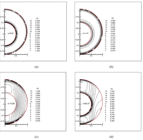
again. As time advances and if the Reynolds number is large, in the corner region between the outer sphere and equator line the angular velocity contours move inwards and those contours in the vicinity of axis of rotation move outwards. This effect can be described by considering the distribution of angular momentum. The rotation of the outer sphere provides a certain amount of angular momentum for the system that by flow in meridian plane and by coriolis forces and nonlinear
advection is redistributed. The fact that the total angular momentum of the azimuthal flow must be conserved by upward and downward moving fluid shows that the rotation of the upward moving elements of fluid (near pole) slow down and rotation of the downward moving elements of fluid (near equator) speeds up. The coriolis forces are bigger in lower hemisphere compared to upper hemisphere because of the eccentricity.
0 0.5 1 -0.75
-0.5 -0.25 0 0.25 0.5 0.75 1
3
4
5
5 6
6 7
7 8
8
8
9
9
10
10
11 11
12
15 6.981E-04
14 5.929E-04
13 4.877E-04
12 3.825E-04
11 2.774E-04
10 1.722E-04
9 6.697E-05
8 -3.823E-05
7 -1.434E-04
6 -2.486E-04
5 -3.538E-04
4 -4.590E-04
3 -5.642E-04
2 -6.694E-04
1 -7.746E-04
ψ
t=0.61
0 0.5 1
-0.75 -0.5 -0.25 0 0.25 0.5 0.75 1
3
5
6 7
7 8
8
9 9
10
11 12 15
15 1.778E-03
14 1.516E-03
13 1.254E-03
12 9.921E-04
11 7.303E-04
10 4.684E-04
9 2.066E-04
8 -5.528E-05
7 -3.171E-04
6 -5.790E-04
5 -8.408E-04
4 -1.103E-03
3 -1.365E-03
2 -1.626E-03
1 -1.888E-03
ψ
t=1.41
(a) (b)
0 0.5 1
-0.75 -0.5 -0.25 0 0.25 0.5 0.75 1
2 534 6 7
8
8
9 10
11
15 2.837E-03
14 2.426E-03
13 2.015E-03
12 1.603E-03
11 1.192E-03
10 7.805E-04
9 3.691E-04
8 -4.230E-05
7 -4.537E-04
6 -8.651E-04
5 -1.276E-03
4 -1.688E-03
3 -2.099E-03
2 -2.511E-03
1 -2.922E-03
ψ
t=15.85
0 0.5 1
-0.75 -0.5 -0.25 0 0.25 0.5 0.75 1
4 5
6
7
8 9 10
11
12
13
15 1.331E-03
14 1.115E-03
13 8.985E-04
12 6.823E-04
11 4.661E-04
10 2.499E-04
9 3.366E-05
8 -1.826E-04
7 -3.988E-04
6 -6.150E-04
5 -8.312E-04
4 -1.047E-03
3 -1.264E-03
2 -1.480E-03
1 -1.696E-03
ψ
t=63.37
(c) (d)
Figure 6. Contours of ψ for Re = 1000, Ωio= -exp(1-t), e = 0.1.
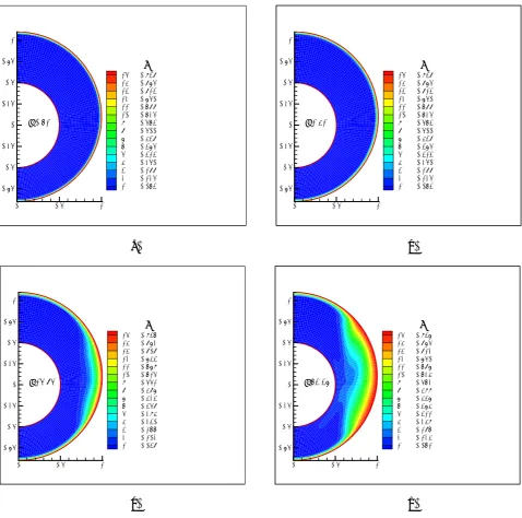
angular velocity of Ωio=−exp(1−t), Re = 1000, Pr = 10, and Ek = 0 are shown in Figures 8 and 9 for the case of e=0.1. At the outset when both spheres dominate the flow, the diffusion of heat from the outer sphere into the field takes place approximately in a steady manner but as the rotation effect of the inner sphere becomes weak, the field temperature grows considerably from the
vicinity of the equator and affects the whole field. This phenomenon is more visible in the lower hemisphere.
0 0.5 1 -0.75
-0.5 -0.25 0 0.25 0.5 0.75 1
5
6
7
9 10
11 12
12 13
13
14
14
15
15 0.949
14 0.787
13 0.624
12 0.462
11 0.300
10 0.138
9 -0.024
8 -0.187
7 -0.349
6 -0.511
5 -0.673
4 -0.836
3 -0.998
2 -1.160
1 -1.322
ω
t=0.61
0 0.5 1
-0.75 -0.5 -0.25 0 0.25 0.5 0.75 1
2
3
5
6 7 8 9
9 10
10
11 12
12 13
13 14 15
15 0.999
14 0.886
13 0.774
12 0.662
11 0.549
10 0.437
9 0.324
8 0.212
7 0.100
6 -0.013
5 -0.125
4 -0.237
3 -0.350
2 -0.462
1 -0.575
ω
t=1.41
(a) (b)
0 0.5 1
-0.75 -0.5 -0.25 0 0.25 0.5 0.75 1
1
2
3
4 5
5
6
6
7
8
9
9
10
11
11
12
12
13 14
15
15 1.036
14 0.960
13 0.885
12 0.810
11 0.734
10 0.659
9 0.583
8 0.508
7 0.433
6 0.357
5 0.282
4 0.207
3 0.131
2 0.056
1 -0.020
ω
t=15.85
0 0.5 1
-0.75 -0.5 -0.25 0 0.25 0.5 0.75 1
1
2
3
7
8
9 10
11
12 13
15 1.042
14 0.972
13 0.903
12 0.833
11 0.764
10 0.694
9 0.625
8 0.556
7 0.486
6 0.417
5 0.347
4 0.278
3 0.208
2 0.139
1 0.069
ω
t=63.37
(c) (d)
Figure 7. Contours of ω for Re = 1000, Ωio= -exp (1-t), e = 0.1.
difference becomes larger because of convection. It is obvious that this difference shows itself in the form of positive and negative numbers. The contours near the pole are negative and the contours near the equator are positive. This is because the clockwise flow which is formed by the rotation of the outer sphere would transfer the heat of this sphere into the field and towards the equator
and the inner sphere.
0 0.5 1 -0.75
-0.5 -0.25 0 0.25 0.5 0.75 1
15 0.938
14 0.875
13 0.813
12 0.750
11 0.688
10 0.625
9 0.563
8 0.500
7 0.438
6 0.375
5 0.313
4 0.250
3 0.188
2 0.125
1 0.063
T
t=0.61
0 0.5 1
-0.75 -0.5 -0.25 0 0.25 0.5 0.75 1
15 0.938
14 0.875
13 0.813
12 0.750
11 0.688
10 0.625
9 0.563
8 0.500
7 0.438
6 0.375
5 0.313
4 0.250
3 0.188
2 0.125
1 0.063
T
t=1.41
(a) (b)
0 0.5 1
-0.75 -0.5 -0.25 0 0.25 0.5 0.75 1
15 0.936
14 0.872
13 0.808
12 0.743
11 0.679
10 0.615
9 0.551
8 0.487
7 0.423
6 0.358
5 0.294
4 0.230
3 0.166
2 0.102
1 0.038
T
t=15.85
0 0.5 1
-0.75 -0.5 -0.25 0 0.25 0.5 0.75 1
15 0.937
14 0.875
13 0.812
12 0.750
11 0.687
10 0.624
9 0.562
8 0.499
7 0.437
6 0.374
5 0.311
4 0.249
3 0.186
2 0.124
1 0.061
T
t=63.37
(c) (d)
Figure 8. Contours of T for Re = 1000, Pr = 10, Ek = 0, Ωio= -exp (1-t), e = 0.1.
conduction case. Again this difference is more visible in lower hemisphere. As evidenced in Figure 8, it is interesting to note that the angular velocities of spheres can cause long delays in heat transfer of the fluid in large areas of the annulus around the poles.
Figures 10 and 11 present the T and (T-Tc)
contours for the same conditions as in Figures 8 and 9 except for Pr = 1. As it is seen in this case,
0 0.5 1 -0.75
-0.5 -0.25 0 0.25 0.5 0.75 1
2 5
6
6
8 9
9 10
10 11
11 12 13
14 15
15 8.498E-03
14 6.085E-03
13 3.673E-03
12 1.261E-03
11 -1.151E-03
10 -3.563E-03
9 -5.976E-03
8 -8.388E-03
7 -1.080E-02
6 -1.321E-02
5 -1.562E-02
4 -1.804E-02
3 -2.045E-02
2 -2.286E-02
1 -2.527E-02
T-Tc
t=0.61
0 0.5 1
-0.75 -0.5 -0.25 0 0.25 0.5 0.75
1 2
23 4
5
5
7
7 8 9
11
12
15 2.978E-02
14 2.305E-02
13 1.633E-02
12 9.612E-03
11 2.891E-03
10 -3.829E-03
9 -1.055E-02
8 -1.727E-02
7 -2.399E-02
6 -3.071E-02
5 -3.743E-02
4 -4.415E-02
3 -5.088E-02
2 -5.760E-02
1 -6.432E-02
T-Tc
t=1.41
(a) (b)
0 0.5 1
-0.75 -0.5 -0.25 0 0.25 0.5 0.75 1
1 2 3
4
5
5 6
6 7
7 8
89 10
11
11
12 13
1415 15
15 2.196E-01
14 1.702E-01
13 1.207E-01
12 7.127E-02
11 2.183E-02
10 -2.761E-02
9 -7.705E-02
8 -1.265E-01
7 -1.759E-01
6 -2.254E-01
5 -2.748E-01
4 -3.243E-01
3 -3.737E-01
2 -4.231E-01
1 -4.726E-01
T-Tc
t=15.85
0 0.5 1
-0.75 -0.5 -0.25 0 0.25 0.5 0.75
1 231
3
4
56
7 8
9
9
10 10
11 11
12
12 13
14
15
15 2.421E-01
14 1.791E-01
13 1.161E-01
12 5.318E-02
11 -9.785E-03
10 -7.275E-02
9 -1.357E-01
8 -1.987E-01
7 -2.616E-01
6 -3.246E-01
5 -3.876E-01
4 -4.505E-01
3 -5.135E-01
2 -5.765E-01
1 -6.394E-01
T-Tc
t=63.37
(c) (d)
Figure 9. Contours of (T-Tc) for Re = 1000, Pr=10, Ek = 0, Ωio= -exp (1-t), e = 0.1.
heat is more visible in lower hemisphere. The difference between Figures 12 and 13 compare to Figures 10 and 11 is in the Eckert number. Eckert number is related to viscous dissipations which are the gradients of velocity that show their effect as a source of heat in energy equation. This source, in fact, expresses the conversion of kinetic energy to heat energy which causes the temperature of the
flow field to rise. This effect (gradients of velocity) is seen in Figure 12 in which the temperature field has more expansion compare to Figure 10. Looking at Figures 13 and 11, this difference is much clearer.
0 0.5 1 -0.75
-0.5 -0.25 0 0.25 0.5 0.75 1
15 0.938
14 0.875
13 0.813
12 0.750
11 0.688
10 0.625
9 0.563
8 0.500
7 0.438
6 0.375
5 0.313
4 0.250
3 0.188
2 0.125
1 0.063
t=0.61
T
0 0.5 1
-0.75 -0.5 -0.25 0 0.25 0.5 0.75 1
15 0.938
14 0.875
13 0.813
12 0.750
11 0.688
10 0.625
9 0.563
8 0.500
7 0.438
6 0.375
5 0.313
4 0.250
3 0.188
2 0.125
1 0.063
t=1.41
T
(a) (b)
0 0.5 1
-0.75 -0.5 -0.25 0 0.25 0.5 0.75 1
15 0.938
14 0.875
13 0.813
12 0.750
11 0.688
10 0.625
9 0.563
8 0.500
7 0.438
6 0.375
5 0.313
4 0.250
3 0.188
2 0.125
1 0.063
t=15.85
T
0 0.5 1
-0.75 -0.5 -0.25 0 0.25 0.5 0.75 1
15 0.938
14 0.875
13 0.813
12 0.750
11 0.688
10 0.625
9 0.563
8 0.500
7 0.438
6 0.375
5 0.313
4 0.250
3 0.188
2 0.125
1 0.063
t=63.37
T
(c) (d)
Figure 10. Contours of T for Re = 1000, Pr = 1, Ek = 0, Ωio = -exp (1-t), e = 0.1.
the vicinity of inner sphere in Figures 13a,b compare to Figures 11a,b. Also, as it is expected, the temperatures are higher when the dissipation terms are not omitted, such as in Ref. 10 and for the case of e = 0.
Figures 14-15 have been drawn for inner angular velocity, t)
2 ( sin 2 io = π
Ω for Re = 1000, Pr
= 10, Ek = 0, for the case of e = 0.1 and in two
consecutive periods (second and third) for the sine function. As known, the sine function oscillates between-1 and 1. In these figures the second and third periods after the sinusoidal movement have been considered. Inner sphere angular velocity in Figures 14a-h is approximately Ωio = 0.0314,
0 0.5 1 -0.75
-0.5 -0.25 0 0.25 0.5 0.75
1 3
4 5
5
6
6 7 8
8 9
10
10 11
11 12
13
15 4.714E-03
14 3.530E-03
13 2.346E-03
12 1.162E-03
11 -2.217E-05
10 -1.206E-03
9 -2.390E-03
8 -3.574E-03
7 -4.758E-03
6 -5.942E-03
5 -7.126E-03
4 -8.310E-03
3 -9.494E-03
2 -1.068E-02
1 -1.186E-02
t=0.61
T-Tc
0 0.5 1
-0.75 -0.5 -0.25 0 0.25 0.5 0.75
1 352
6 7
7 8
8 9
10
10
11
12 13
14
15 2.067E-02
14 1.554E-02
13 1.040E-02
12 5.266E-03
11 1.317E-04
10 -5.003E-03
9 -1.014E-02
8 -1.527E-02
7 -2.041E-02
6 -2.554E-02
5 -3.068E-02
4 -3.581E-02
3 -4.095E-02
2 -4.608E-02
1 -5.122E-02
t=1.41
T-Tc
(a) (b)
0 0.5 1
-0.75 -0.5 -0.25 0 0.25 0.5 0.75 1
1
1 4
4 5
5 7
7 8
9 9
10
10
11
11
12
12
13 14
15 2.417E-01
14 1.935E-01
13 1.454E-01
12 9.717E-02
11 4.897E-02
10 7.836E-04
9 -4.741E-02
8 -9.560E-02
7 -1.438E-01
6 -1.920E-01
5 -2.402E-01
4 -2.884E-01
3 -3.366E-01
2 -3.847E-01
1 -4.329E-01
t=15.85
T-Tc
0 0.5 1
-0.75 -0.5 -0.25 0 0.25 0.5 0.75 1
2 4
56 7
8
8 10
10
11
12
13
14
15 2.321E-01
14 1.791E-01
13 1.262E-01
12 7.331E-02
11 2.039E-02
10 -3.253E-02
9 -8.545E-02
8 -1.384E-01
7 -1.913E-01
6 -2.442E-01
5 -2.971E-01
4 -3.500E-01
3 -4.030E-01
2 -4.559E-01
1 -5.088E-01
t=63.37
T-Tc
(c) (d)
Figure 11. Contours of (T-Tc) for Re = 1000, Pr = 1, Ek = 0, Ωio = -exp (1-t), e = 0.1.
has come to an important change, meaning that it has been considered immediately after a change of acceleration.
For example, for the time value between the case (a) and just before the case (b) the inner sphere acceleration is positive and the time value at (b) is the starting point of negative acceleration for this sphere. As it is seen from Figure 15, the
0 0.5 1 -0.75
-0.5 -0.25 0 0.25 0.5 0.75 1
15 0.938
14 0.875
13 0.813
12 0.750
11 0.688
10 0.625
9 0.563
8 0.500
7 0.438
6 0.375
5 0.313
4 0.250
3 0.188
2 0.125
1 0.063
t=0.61
T
0 0.5 1
-0.75 -0.5 -0.25 0 0.25 0.5 0.75 1
15 0.938
14 0.875
13 0.813
12 0.750
11 0.688
10 0.625
9 0.563
8 0.500
7 0.438
6 0.375
5 0.313
4 0.250
3 0.188
2 0.125
1 0.063
t=1.41
T
(a) (b)
0 0.5 1
-0.75 -0.5 -0.25 0 0.25 0.5 0.75 1
15 0.938
14 0.875
13 0.813
12 0.750
11 0.688
10 0.625
9 0.563
8 0.500
7 0.438
6 0.375
5 0.313
4 0.250
3 0.188
2 0.125
1 0.063
t=15.85
T
0 0.5 1
-0.75 -0.5 -0.25 0 0.25 0.5 0.75 1
15 0.938
14 0.875
13 0.813
12 0.750
11 0.688
10 0.625
9 0.563
8 0.500
7 0.438
6 0.375
5 0.313
4 0.250
3 0.188
2 0.125
1 0.063
t=63.37
T
(c) (d)
Figure 12. Contours of T for Re = 1000, Pr = 1, Ek = 0.001, Ωio= -exp (1-t), e = 0.1.
of the previous period the inner sphere has negative angular velocity. Therefore, as the outer sphere containing a constant velocity has a continuous and steady effect on the entire flow field, the inner sphere having an oscillating velocity between-2 and 2 (periodic acceleration of positive and negative) induces an unsteady and oscillatory type of effect on the layers in the
vicinity of the inner sphere. Also, the effect of eccentricity clearly portrays the un-symmetric situation in these figures.
(T-0 0.5 1 -0.75
-0.5 -0.25 0 0.25 0.5 0.75 1
2
2
2
3
3
3
3 4
4
4
5
5
5 6
6 7
7
7
8
8
8
9
9
9
10
10
11
11
12
12
13
14 15
15 9.838E-02
14 9.097E-02
13 8.356E-02
12 7.614E-02
11 6.873E-02
10 6.132E-02
9 5.390E-02
8 4.649E-02
7 3.908E-02
6 3.166E-02
5 2.425E-02
4 1.684E-02
3 9.426E-03
2 2.013E-03
1 -5.400E-03
t=0.61
T-Tc
0 0.5 1
-0.75 -0.5 -0.25 0 0.25 0.5 0.75 1
2 3 5
5
5 5
6 6
6
7 7
7
8
8
9
9
10 11
12
13 14
15 1.197E-01
14 1.080E-01
13 9.625E-02
12 8.454E-02
11 7.284E-02
10 6.113E-02
9 4.942E-02
8 3.771E-02
7 2.601E-02
6 1.430E-02
5 2.592E-03
4 -9.115E-03
3 -2.082E-02
2 -3.253E-02
1 -4.424E-02
t=1.41
T-Tc
(a) (b)
0 0.5 1
-0.75 -0.5 -0.25 0 0.25 0.5 0.75 1
3
4 5
5 6
6 7
8 9
9
10 10
11
12
12
13
13
15 3.184E-01
14 2.653E-01
13 2.121E-01
12 1.589E-01
11 1.057E-01
10 5.257E-02
9 -6.043E-04
8 -5.378E-02
7 -1.070E-01
6 -1.601E-01
5 -2.133E-01
4 -2.665E-01
3 -3.196E-01
2 -3.728E-01
1 -4.260E-01
t=15.85
T-Tc
0 0.5 1
-0.75 -0.5 -0.25 0 0.25 0.5 0.75 1
2
3
3 7
8 9
10
10 11
11 12
1314
15 2.716E-01
14 2.173E-01
13 1.631E-01
12 1.089E-01
11 5.469E-02
10 4.737E-04
9 -5.374E-02
8 -1.080E-01
7 -1.622E-01
6 -2.164E-01
5 -2.706E-01
4 -3.248E-01
3 -3.790E-01
2 -4.333E-01
1 -4.875E-01
t=63.37
T-Tc
(c) (d)
Figure 13. Contours of (T-Tc) for Re = 1000, Pr = 1, Ek = 0.001, Ωio= -exp (1-t), e = 0.1.
Tc) contours for the inner angular velocity of
) t 2 ( sin 2 io = π
Ω are depicted in Figures 16 and 17 for Re = 1000, Pr = 10, and Ek = 0. Similar types of discussions as in Figures 8 and 9 apply here as well. Also the delay in heat transfer of the fluid in large portions of annulus can be seen in Figure 16.
Again, the profiles show that because of the eccentricity the coriolis force in lower hemisphere is bigger than the upper hemisphere and therefore it worms up faster.
0 0.5 1 -0.75
-0.5 -0.25 0 0.25 0.5 0.75 1
3 4
5 6
6 7
7
8
8
9
10
11
12
13 15 6.589E-03
14 5.816E-03
13 5.043E-03
12 4.269E-03
11 3.496E-03
10 2.723E-03
9 1.950E-03
8 1.177E-03
7 4.039E-04
6 -3.692E-04
5 -1.142E-03
4 -1.915E-03
3 -2.688E-03
2 -3.462E-03
1 -4.235E-03
ψ
t=4.01
0 0.5 1
-0.75 -0.5 -0.25 0 0.25 0.5 0.75 1
4
5
6
7
8
9
10 11 12
15 7.648E-03
14 6.748E-03
13 5.849E-03
12 4.950E-03
11 4.051E-03
10 3.152E-03
9 2.253E-03
8 1.354E-03
7 4.546E-04
6 -4.445E-04
5 -1.344E-03
4 -2.243E-03
3 -3.142E-03
2 -4.041E-03
1 -4.940E-03
ψ
t=5.01
(a) (b)
0 0.5 1
-0.75 -0.5 -0.25 0 0.25 0.5 0.75 1
3
4
5 6
6
7
8
9
10 14 12 15
15 7.971E-03
14 7.052E-03
13 6.132E-03
12 5.213E-03
11 4.293E-03
10 3.374E-03
9 2.454E-03
8 1.535E-03
7 6.154E-04
6 -3.041E-04
5 -1.224E-03
4 -2.143E-03
3 -3.063E-03
2 -3.982E-03
1 -4.902E-03
ψ
t=6.01
0 0.5 1
-0.75 -0.5 -0.25 0 0.25 0.5 0.75 1
4
6 7
8 9
12
13
15 7.694E-03
14 6.816E-03
13 5.937E-03
12 5.058E-03
11 4.179E-03
10 3.300E-03
9 2.421E-03
8 1.542E-03
7 6.632E-04
6 -2.158E-04
5 -1.095E-03
4 -1.974E-03
3 -2.853E-03
2 -3.731E-03
1 -4.610E-03
ψ
t=7.01
(c) (d)
0 0.5 1
-0.75 -0.5 -0.25 0 0.25 0.5 0.75 1
2 3 5
5 6
7 8
11 12
15 7.019E-03
14 6.233E-03
13 5.446E-03
12 4.659E-03
11 3.872E-03
10 3.085E-03
9 2.298E-03
8 1.511E-03
7 7.241E-04
6 -6.281E-05
5 -8.497E-04
4 -1.637E-03
3 -2.424E-03
2 -3.211E-03
1 -3.997E-03
ψ
t=8.01
0 0.5 1
-0.75 -0.5 -0.25 0 0.25 0.5 0.75 1
1 3 6
6
7 8
9
10 11
13
15 6.384E-03
14 5.670E-03
13 4.957E-03
12 4.243E-03
11 3.529E-03
10 2.816E-03
9 2.102E-03
8 1.389E-03
7 6.752E-04
6 -3.840E-05
5 -7.520E-04
4 -1.466E-03
3 -2.179E-03
2 -2.893E-03
1 -3.606E-03
ψ
t=9.01
0 0.5 1 -0.75
-0.5 -0.25 0 0.25 0.5 0.75 1
2
4 5
5 6
7
8
13 15 5.789E-03
14 5.150E-03
13 4.512E-03
12 3.874E-03
11 3.236E-03
10 2.598E-03
9 1.960E-03
8 1.322E-03
7 6.836E-04
6 4.552E-05
5 -5.926E-04
4 -1.231E-03
3 -1.869E-03
2 -2.507E-03
1 -3.145E-03
ψ
t=10.01
0 0.5 1
-0.75 -0.5 -0.25 0 0.25 0.5 0.75 1
5
6
6 7
9 13
15 5.130E-03
14 4.563E-03
13 3.995E-03
12 3.427E-03
11 2.859E-03
10 2.292E-03
9 1.724E-03
8 1.156E-03
7 5.886E-04
6 2.085E-05
5 -5.469E-04
4 -1.115E-03
3 -1.682E-03
2 -2.250E-03
1 -2.818E-03
ψ
t=11.01
(g) (h)
Figure 14. Contours of ψ for Re = 1000, Pr = 10, Ek = 0, Ωio = 2sin(πt/2), e = 0.1.
0 0.5 1
-0.75 -0.5 -0.25 0 0.25 0.5 0.75 1
1
2
3
3
5
6
7
8
9
10
11 12
12
13 15 1.112
14 1.003
13 0.893
12 0.784
11 0.674
10 0.565
9 0.455
8 0.346
7 0.236
6 0.127
5 0.017
4 -0.092
3 -0.202
2 -0.311
1 -0.421
ω
t=4.01
0 0.5 1
-0.75 -0.5 -0.25 0 0.25 0.5 0.75 1
1
2
3
3 4
5
5
6 6
7
7
8 10
11
4
15 1.872
14 1.743
13 1.615
12 1.487
11 1.359
10 1.231
9 1.102
8 0.974
7 0.846
6 0.718
5 0.589
4 0.461
3 0.333
2 0.205
1 0.077
ω
t=5.01
(a) (b)
0 0.5 1
-0.75 -0.5 -0.25 0 0.25 0.5 0.75 1
1 1
2
2
2
3
3
4
4
4
5
5 6
67 7
8 9
10 11
12
13
15 1.145
14 1.067
13 0.990
12 0.913
11 0.835
10 0.758
9 0.680
8 0.603
7 0.526
6 0.448
5 0.371
4 0.294
3 0.216
2 0.139
1 0.062
ω
t=6.01
0 0.5 1
-0.75 -0.5 -0.25 0 0.25 0.5 0.75 1
2
5
9
10 10
11
12
13
14
15 1.021
14 0.819
13 0.618
12 0.416
11 0.215
10 0.014
9 -0.188
8 -0.389
7 -0.590
6 -0.792
5 -0.993
4 -1.194
3 -1.396
2 -1.597
1 -1.799
ω
t=7.01
0 0.5 1 -0.75
-0.5 -0.25 0 0.25 0.5 0.75 1
2
3
3 4
5 6
7 8
9
10
11
12 13
15 1.111
14 1.001
13 0.890
12 0.780
11 0.669
10 0.559
9 0.448
8 0.338
7 0.227
6 0.117
5 0.006
4 -0.104
3 -0.215
2 -0.325
1 -0.436
ω
t=8.01
0 0.5 1
-0.75 -0.5 -0.25 0 0.25 0.5 0.75 1
1
1
2 3
4
4
5
6
7
7 8 9
10
11
12
13 15
15 1.872
14 1.744
13 1.615
12 1.487
11 1.359
10 1.231
9 1.103
8 0.975
7 0.846
6 0.718
5 0.590
4 0.462
3 0.334
2 0.206
1 0.077
ω
t=9.01
(e) (f)
0 0.5 1
-0.75 -0.5 -0.25 0 0.25 0.5 0.75
1 1
2
2 3
4
5
5 5
6 7 7
8 8
9
10
11
12
13
15 1.146
14 1.071
13 0.996
12 0.920
11 0.845
10 0.769
9 0.694
8 0.618
7 0.543
6 0.467
5 0.392
4 0.316
3 0.241
2 0.165
1 0.090
ω
t=10.01
0 0.5 1
-0.75 -0.5 -0.25 0 0.25 0.5 0.75 1
2 3
5
7 10
11
12
13
14
15 1.021
14 0.819
13 0.618
12 0.416
11 0.215
10 0.014
9 -0.188
8 -0.389
7 -0.590
6 -0.792
5 -0.993
4 -1.194
3 -1.396
2 -1.597
1 -1.799
ω
t=11.01
(g) (h)
Figure 15. Contours of ω for Re = 1000, Pr = 10, Ek = 0, Ωio = 2sin(πt/2), e = 0.1.
0 0.5 1
-0.75 -0.5 -0.25 0 0.25 0.5 0.75 1
15 0.936
14 0.872
13 0.809
12 0.745
11 0.681
10 0.617
9 0.554
8 0.490
7 0.426
6 0.362
5 0.299
4 0.235
3 0.171
2 0.107
1 0.044
T
t=4.01
0 0.5 1
-0.75 -0.5 -0.25 0 0.25 0.5 0.75 1
15 0.936
14 0.872
13 0.808
12 0.744
11 0.680
10 0.616
9 0.552
8 0.487
7 0.423
6 0.359
5 0.295
4 0.231
3 0.167
2 0.103
1 0.039
T
t=5.01
0 0.5 1 -0.75
-0.5 -0.25 0 0.25 0.5 0.75 1
15 0.936
14 0.871
13 0.807
12 0.743
11 0.679
10 0.614
9 0.550
8 0.486
7 0.422
6 0.357
5 0.293
4 0.229
3 0.165
2 0.100
1 0.036
T
t=6.01
0 0.5 1
-0.75 -0.5 -0.25 0 0.25 0.5 0.75 1
15 0.936
14 0.871
13 0.807
12 0.743
11 0.678
10 0.614
9 0.550
8 0.485
7 0.421
6 0.357
5 0.292
4 0.228
3 0.163
2 0.099
1 0.035
T
t=7.01
(c) (d)
0 0.5 1
-0.75 -0.5 -0.25 0 0.25 0.5 0.75 1
15 0.936
14 0.871
13 0.807
12 0.742
11 0.678
10 0.614
9 0.549
8 0.485
7 0.420
6 0.356
5 0.292
4 0.227
3 0.163
2 0.098
1 0.034
T
t=8.01
0 0.5 1
-0.75 -0.5 -0.25 0 0.25 0.5 0.75 1
15 0.936
14 0.871
13 0.807
12 0.742
11 0.678
10 0.614
9 0.549
8 0.485
7 0.420
6 0.356
5 0.291
4 0.227
3 0.163
2 0.098
1 0.034
T
t=9.01
(e) (f)
0 0.5 1
-0.75 -0.5 -0.25 0 0.25 0.5 0.75 1
15 0.936
14 0.871
13 0.807
12 0.742
11 0.678
10 0.613
9 0.549
8 0.485
7 0.420
6 0.356
5 0.291
4 0.227
3 0.162
2 0.098
1 0.034
T
t=10.01
0 0.5 1
-0.75 -0.5 -0.25 0 0.25 0.5 0.75 1
15 0.936
14 0.871
13 0.807
12 0.742
11 0.678
10 0.613
9 0.549
8 0.485
7 0.420
6 0.356
5 0.291
4 0.227
3 0.162
2 0.098
1 0.033
T
t=11.01
(g) (h)
0 0.5 1 -0.75
-0.5 -0.25 0 0.25 0.5 0.75
1 3 4
6
6 7 8
8 9
9
10 11
11
12
14
15 1.003E-01
14 7.497E-02
13 4.961E-02
12 2.426E-02
11 -1.099E-03
10 -2.645E-02
9 -5.181E-02
8 -7.716E-02
7 -1.025E-01
6 -1.279E-01
5 -1.532E-01
4 -1.786E-01
3 -2.039E-01
2 -2.293E-01
1 -2.546E-01
t=4.01
T-Tc
0 0.5 1
-0.75 -0.5 -0.25 0 0.25 0.5 0.75
1 5 36
6
7
7
8
8 9
10
10
11
12
13
15
15 1.256E-01
14 9.558E-02
13 6.553E-02
12 3.548E-02
11 5.432E-03
10 -2.462E-02
9 -5.467E-02
8 -8.471E-02
7 -1.148E-01
6 -1.448E-01
5 -1.749E-01
4 -2.049E-01
3 -2.350E-01
2 -2.650E-01
1 -2.951E-01
t=5.01
T-Tc
(a) (b)
0 0.5 1
-0.75 -0.5 -0.25 0 0.25 0.5 0.75
14 3
4 6 7
7
8
8 9
9 10
11
11 14
15 1.441E-01
14 1.104E-01
13 7.661E-02
12 4.285E-02
11 9.085E-03
10 -2.468E-02
9 -5.844E-02
8 -9.220E-02
7 -1.260E-01
6 -1.597E-01
5 -1.935E-01
4 -2.272E-01
3 -2.610E-01
2 -2.948E-01
1 -3.285E-01
t=6.01
T-Tc
0 0.5 1
-0.75 -0.5 -0.25 0 0.25 0.5 0.75
1 2
3
5
6 7
7
8 9
9
10
10
11
12
13
14
15
15 1.567E-01
14 1.200E-01
13 8.332E-02
12 4.664E-02
11 9.965E-03
10 -2.671E-02
9 -6.339E-02
8 -1.001E-01
7 -1.367E-01
6 -1.734E-01
5 -2.101E-01
4 -2.468E-01
3 -2.834E-01
2 -3.201E-01
1 -3.568E-01
t=7.01
T-Tc
(c) (d)
0 0.5 1
-0.75 -0.5 -0.25 0 0.25 0.5 0.75
1 1 2
4 5
5
6
7
7 8
8 9
9 10
10
11
12
13 14
15 1.678E-01
14 1.286E-01
13 8.940E-02
12 5.020E-02
11 1.100E-02
10 -2.820E-02
9 -6.740E-02
8 -1.066E-01
7 -1.458E-01
6 -1.850E-01
5 -2.242E-01
4 -2.634E-01
3 -3.026E-01
2 -3.418E-01
1 -3.810E-01
t=8.01
T-Tc
0 0.5 1
-0.75 -0.5 -0.25 0 0.25 0.5 0.75 1
4
5
5 6
6 7
7
8
8
9
9 10 10
10 11
12
13
15
15 1.722E-01
14 1.312E-01
13 9.015E-02
12 4.912E-02
11 8.096E-03
10 -3.293E-02
9 -7.396E-02
8 -1.150E-01
7 -1.560E-01
6 -1.970E-01
5 -2.381E-01
4 -2.791E-01
3 -3.201E-01
2 -3.611E-01
1 -4.022E-01
t=9.01
T-Tc
0 0.5 1 -0.75
-0.5 -0.25 0 0.25 0.5 0.75
1 3
4 5
5 6
7
7
8
8 9
9
10
10 11
12 13 15
15 1.679E-01
14 1.259E-01
13 8.399E-02
12 4.203E-02
11 7.216E-05
10 -4.189E-02
9 -8.385E-02
8 -1.258E-01
7 -1.678E-01
6 -2.097E-01
5 -2.517E-01
4 -2.936E-01
3 -3.356E-01
2 -3.776E-01
1 -4.195E-01
t=10.01
T-Tc
0 0.5 1
-0.75 -0.5 -0.25 0 0.25 0.5 0.75
1 3
3
4
4 5
5 6
6
7
7
8
8 9
9
10
10 11
11 12
13 14
15 1.753E-01
14 1.316E-01
13 8.783E-02
12 4.407E-02
11 3.134E-04
10 -4.344E-02
9 -8.720E-02
8 -1.310E-01
7 -1.747E-01
6 -2.185E-01
5 -2.622E-01
4 -3.060E-01
3 -3.497E-01
2 -3.935E-01
1 -4.372E-01
t=11.01
T-Tc
(g) (h)
Figure 17. Contours of (T-Tc) for Re = 1000, Pr = 10, Ek = 0, Ωio = 2sin(πt/2), e = 0.1.
0 0.5 1
-0.75 -0.5 -0.25 0 0.25 0.5 0.75 1
1 2
3
4
5
6
7
7
8
8
9
9
10
11 12
13 1514 1.612E-031.398E-03
13 1.185E-03
12 9.711E-04
11 7.575E-04
10 5.440E-04
9 3.304E-04
8 1.168E-04
7 -9.679E-05
6 -3.104E-04
5 -5.240E-04
4 -7.375E-04
3 -9.511E-04
2 -1.165E-03
1 -1.378E-03
t=63.37
ψ
0 0.5 1
-0.75 -0.5 -0.25 0 0.25 0.5 0.75 1
1
2
4
5 6
7
7
8
8 9
10
10
11
12
13
13
14
14
15 1.036
14 0.967
13 0.898
12 0.829
11 0.760
10 0.691
9 0.622
8 0.553
7 0.483
6 0.414
5 0.345
4 0.276
3 0.207
2 0.138
1 0.069
t=63.37
ω
(a) (b)
0 0.5 1
-0.75 -0.5 -0.25 0 0.25 0.5 0.75 1
15 0.937
14 0.874
13 0.812
12 0.749
11 0.686
10 0.623
9 0.561
8 0.498
7 0.435
6 0.372
5 0.309
4 0.247
3 0.184
2 0.121
1 0.058
t=63.37
T
0 0.5 1
-0.75 -0.5 -0.25 0 0.25 0.5 0.75 1
1
2
3
4 5
6 7
7 8
10 10
11 12
13
15
15 4.046E-01
14 3.290E-01
13 2.533E-01
12 1.776E-01
11 1.020E-01
10 2.628E-02
9 -4.938E-02
8 -1.251E-01
7 -2.007E-01
6 -2.764E-01
5 -3.521E-01
4 -4.277E-01
3 -5.034E-01
2 -5.791E-01
1 -6.547E-01
t=63.37
T-Tc
(c) (d)
0 0.5 1 -0.75
-0.5 -0.25 0 0.25 0.5 0.75 1
1 4
5
6
6 6
7
7
7 8
910 1112
15 4.546E-03
14 3.981E-03
13 3.416E-03
12 2.851E-03
11 2.286E-03
10 1.721E-03
9 1.156E-03
8 5.913E-04
7 2.641E-05
6 -5.385E-04
5 -1.103E-03
4 -1.668E-03
3 -2.233E-03
2 -2.798E-03
1 -3.363E-03
t=11.01
ψ
0 0.5 1
-0.75 -0.5 -0.25 0 0.25 0.5 0.75 1
1
3
4
5
6
8
11
11 12
13
14
15
15 0.911
14 0.717
13 0.523
12 0.329
11 0.135
10 -0.059
9 -0.253
8 -0.447
7 -0.642
6 -0.836
5 -1.030
4 -1.224
3 -1.418
2 -1.612
1 -1.806
t=11.01
ω
(a) (b)
0 0.5 1
-0.75 -0.5 -0.25 0 0.25 0.5 0.75 1
15 0.936
14 0.871
13 0.807
12 0.743
11 0.679
10 0.614
9 0.550
8 0.486
7 0.422
6 0.357
5 0.293
4 0.229
3 0.164
2 0.100
1 0.036
t=11.01
T
0 0.5 1
-0.75 -0.5 -0.25 0 0.25 0.5 0.75 1
2 3
3 4
4 5
6
6 7
9
9
10
11
12 13
14
15 1.749E-01
14 1.364E-01
13 9.782E-02
12 5.927E-02
11 2.073E-02
10 -1.782E-02
9 -5.637E-02
8 -9.491E-02
7 -1.335E-01
6 -1.720E-01
5 -2.106E-01
4 -2.491E-01
3 -2.876E-01
2 -3.262E-01
1 -3.647E-01
t=11.01
T-Tc
(c) (d)
Figure 19. Flow and heat transfer for Re = 1000, Pr = 10, Ek = 0, Ωio= 2sin(πt/2), e = 0.05.
5. CONCLUSIONS
A numerical study of flow and heat transfer of a viscous incompressible fluid within a rotating spherical annulus have been investigated when the spheres have time-dependent prescribed values of angular velocities. The characteristics of the flow
At small Reynolds numbers the secondary flow or the vortices which cause forced convection, are small values and thus the effect of convectivity and therefore the intensity of their local heat transfer is not too different from the pure conduction. But for large Reynolds numbers some deviations are seen in angular velocity and temperature distributions which is an indication of the effect of secondary flow on the primary flow. Since we have considered the case with time-dependent angular velocities then the relative velocities of the spheres are functions of time.
Applying these angular velocities, shear layers are formed in the vicinity of the spheres which get thicker because of viscous diffusion effect and depending on the flow conditions one or two circulations are formed in meridian plane. Interesting effect of long delays in heat transfer of a large portion of the fluid in the annulus is observed because of the angular velocities of the corresponding spheres. As the eccentricity increases and the gap between the spheres decreases, the coriolis forces and convection heat transfer effect in the narrower portion increase.
6. REFERENCES
1. Howarth, L., “Note on Boundary Layer on a Rotating Sphere”, Philosophy Magazine Series, Vol. 7, No. 42,
(1951), 1308-1311.
2. Proudman, I., “The Almost-Rigid Rotation of Viscous Fluid Between Concentric Spheres”, Journal of Fluid Mechanics, Vol. 1, (1956), 505-516.
3. Lord, R. G. and Bowden, F. P., “Boundary Layer on a Rotating Sphere”, Proceeding of Royal Society, Vol. A
271, (1963), 143-146.
4. Fox, J., “Singular Perturbation of Viscous Fluid Between Spheres”, NASA TN D-2491, (1964), 1-50.
5. Greenspan, H. P., “Axially Symmetric Motion of a Rotating Fluid in a Spherical Annulus”, Journal of Fluid Mechanics, Vol. 21, (1964), 673-677.
6. Carrier, G. F., “Some Effects of Stratification and
Geometry in Rotating Fluids”, Journal of Fluid Mechanics, Vol. 24, (1966), 641-659.
7. Stewartson, K., “On Almost Rigid Rotations Part 2”,
Journal of Fluid Mechanics, Vol. 26, (1966), 131-144.
8. Pearson, C., A., “Numerical Study of the Time-Dependent Viscous Flow Between Two Rotating Spheres”, Journal of Fluid Mechanics, Vol. 28, (1967),
323-336.
9. Munson, B. R. and Joseph, D. D., “Viscous Incompressible Flow Between Concentric Rotating Spheres, Part I: Basic Flow”, Journal of Fluid Mechanics, Vol. 49, (1971), 289-303.
10. Douglass, R. W., Munson, B. R. and Shaughnessy, E. J., “Thermal Convection in Rotating Spherical Annuli-1. Forced Convection”, Int. J. Heat and Mass Transfer,
Vol. 21, (1978), 1543-1553.
11. Munson, B. R. and Douglass, R. W., “Viscous Flow in Oscillatory Spherical Annuli”, Journal of Physics of Fluids, Vol. 22, No. 2, (February 1979), 205-208.
12. Gagliardi, J. C., Nigro, N. J., Elkouh, A. F., and Yang, J. K., “Study of the Axially Symmetric Motion of an Incompressible Viscous Fluid Between Two Concentric Rotating Spheres”, Journal of Engineering Mathematics, Vol. 24, (1990), 1-23.
13. Yang, J.-K., Nigro, N. J. and Elkouh, A. F., “Numerical Study the Axially Symmetric Motion of an Incompressible Viscous Fluid in an Annulus Between Two Concentric Rotating Spheres”, International Journal for Numerical Methods in Fluids, Vol. 9,
(1989), 689-712.
14. Ni, W. and Nigro, N. J., “Finite Element Analysis of the Axially Symmetric Motion of an Incompressible Viscous Fluid in a Spherical Annulus”, International Journal for Numerical Methods in Fluids, Vol. 19,
(1994), 207-236.
15. Jabari Moghadam, A. and Baradaran Rahimi, A., “Similarity Solution in Study of Flow and Heat Transfer Between Two Rotating Spheres with Constant Angular Velocities”, Accepted for Publication in Journal of Scientia Iranica, Sharif Univ. of Tech., Tehran, Iran,
(2008).
16. Jabari Moghadam, A. and Baradaran Rahimi, A., “A Numerical Study of Flow and Heat Transfer Between Two Rotating Spheres with Time-Dependent Angular Velocities”, Accepted for Publication in Journal of Heat Transfer, Transaction of ASME, Vol. 130, (July
2008), 1-9.
![TABLE 1. Results of References [8-10] for Re = 50, Ωio = -3, and Pr = 10.](https://thumb-us.123doks.com/thumbv2/123dok_us/241264.2018840/7.595.48.540.104.465/table-results-references-io-pr.webp)