Tracking and Shape Control of a Micro-cantilever using Electrostatic Actuation

Please cite this article as: F. Karami, H. Salarieh, R. Shabani, Tracking and Shape Control of a Micro-cantilever using Electrostatic Actuation, International Journal of Engineering (IJE), TRANSACTIONS C: Aspects Vol. 27, No. 9, (September 2014) 1439-1448

International Journal of Engineering

J o u r n a l H o m e p a g e : w w w . i j e . i r

Tracking and Shape Control of a Micro-cantilever using Electrostatic Actuation

F. Karamia_{, H. Salarieh*} a_{, R. Shabani}b

a _{Department of Mechanical Engineering, Sharif University of Technology, Tehran, Iran} b_{Department of Mechanical Engineering, Faculty of Engineering, Urmia University, Urmia, Iran}

P A P E R I N F O

Paper history:

Received 02 November 2013 Received in revised form 14 May 2014 Accepted 22 May 2014

Keywords:

Micro-cantilever Electrostatic Actuation State Estimation Tracking Control Shape Control

A B S T R A C T

In this paper, the problems of state estimation, tracking control and shape control in a micro-cantilever beam with nonlinear electrostatic actuation are investigated. The system’s partial differential equation of motion is converted into a set of ordinary differential equations by projection method. Observabillity of the system is proven and a state estimation system is designed using extended Kalman filter (EKF) algorithm. A tracking control system is designed to make a specific point of the beam follow a reference signal. The effect of mode selection to include in model on controller performance is also investigated. Based on the tracking controller a shape control algorithm is designed to form the shape of beam into a desired shape. The proposed algorithms are validated by numerical simulation and resulted in a promising performance.

doi:10.5829/idosi.ije.2014.27.09c.14

1. INTRODUCTION 1

MEMS systems have drawn growing attention in sensing and actuating fields, recently. Using electrostatic force is the most frequent actuating and sensing method in MEMS because of its simple structure, simple manufacturing and high efficiency. Microbeams are the most common structures that used in MEMS systems. They are the backbone of many MEMS devices, Younis [1]. The combination of the electrostatic actuation and microbeam structure has many applications in industrial and scientific fields like mass sensing systems, micro pressure sensors, micro flexible joints and ink injection printers as presented by Seoka [2], Kamisuki [3], Chu et al. [4], Hassanpour et al. [5], Takashi et al. [6] and Chau et al. [7], Gangi et al. [8].

Some other works have considered dynamics of the system. Some papers were dedicated to deriving equation of motion for electrostatically actuated beams, while some others consider their vibration as

1

*Corresponding Author's Email: [email protected] (H. Salarieh)

Rahman et al. [9], Brusa et al. [10], Batra [11], Mojahedi et al. [12], Abbasnejad et al. [13]. Pull-in instability also has drawn much attention in the literature. Numerous works are dedicated to predict pull-in voltage and its properties like Rezazadeh et al. [14], Ganji [15] and Lakard et al. [16].

1

V+

1

V−

2

V−

2

V+

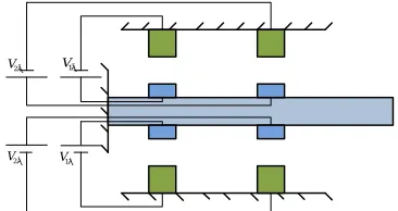
Figure 1. An electrostatically actuated micro-cantilever

In addition to electrostatic actuation, there are some works deal with vibration control of beams using piezo electric actuators. Optimal vibration control of beams using piezo electric actuation is presented by Kucuk et al. [22].

Shape control is an algorithm which made shape of a structure change into a specific one by means of actuators. Most common application of shape control in micro scale is in adaptive optic systems. Electrostatically actuated microsystems have wide applications in adaptive optic systems like deformable mirrors. Many studies are dedicated to fabrication and implementation of these systems as Huaet al. [23], Bonora [24], Cugata et al. [25], but controller design is not investigated widely. There are new trends in MEMS and Nano scale studies which focused on the effect of structure size in dynamics of small scale systems. The main scope of the paper is control and observer design for a micro scale system and authors tried to elaborate methods which can be used to control the shape of any micro structures. The modeling of Micro and Nano systems by nonclassic methods are investigated widely in the literature. For example, implementing of a simple regulator to suppress the vibration of a beam is presented in another work by the authors [26].

As mentioned before, works that dealt with controller design mainly used lumped parameter models. On the other hand, few works which used distributed parameter models include significant simplification of nonlinear nature of the excitation terms. Present work intends to avoid any significant simplifications and take the distributed parameters and nonlinearity into account to design a reliable and effective controller-observer system. The actuation term in the equation of motion that introduced significant nonlinearity into the equations is fully taken into account to avoid misunderstanding due to over simplification of equations. Using the developed comprehensive dynamic model, a control system is designed to ensure tracking of a reference signal for some points of the beam and based on the designed tracking control system an innovative shape control scheme is proposed to transform the microbeam into a desired shape. The main goal of this work is designing a

nonlinear controller without any prominent simplification and linearization, and also proposing a new shape control algorithm. A state observation system is also designed to estimate the states which are needed in control system. Due to technological restrictions in micro scale, reliable estimation of the states is vital to control and stabilization tasks. This system should estimatethe states by the least measurements to fit limits of implementation and fabrication in micro scale.

2. DYNAMIC MODEL

The studied system is composed of a narrow, long and flexible cantilever beam that is subjected to electrostatic force via some electrodes. The actuators are modeled as separate electrodes. This configuration permits the use of multi input control algorithm. The electrostatic actuation is naturally unidirectional force and an actuator is only able to attract the beam not to drive it back. Thus, to exert force in two directions, actuators must be placed on both sides of the beam. It is necessary for control action that makes the beam move on both sides of its rest position. In Figure 1, the proposed combination is shown. Magnitude of the electrostatic force is obtained by the following Equations (1):

( )

(

)

( )

(

)

2

, 2

2

, 2

( ) ( )

1

2 _,

( ) ( )

1

2 _,

i i elec l

i i elec u

x V t

F b or

g w x t

x V t

F b

g w x t

ψ ε

ψ ε

+

−

=

−

= −

+

(1)

where ε, b and g are vacuum permittivity, width of the beam and initial gap between the beam and the electrode, respectively. They are the characteristic function of the actuator effectiveness in spatial domain. This function weights the effect of electrostatic actuation on predetermined points of the beam. It is supposed that actuation only affects on the points located directly above or below the actuators. Therefore, the pulse function can be used for ψ. V is the applied voltage and w is the lateral displacement of the beam. The first equation pertains to actuators placed below the beam and the second equation to above actuators. The voltage of electrodes placed below the beam is denoted by V+ and the electrodes placed above the beam are

denoted by V-. Since a pair of opposite electrodes plays

as single bidirectional actuator with capability of attraction/repulsion, we have in every time onlyV+or V-,

not both of them. Using Euler-Bernoulli model of beam and electrostatic actuation term of Equation (1) leads to the following equation as general equation of motion.

( )

(

)

(

( )

)

4 2

4 2

2 2

2 2

1 1

( , ) ( , )

( ) ( ) ( ) ( )

1

2 _{, ,}

N N

i i i i

i i

w x t w x t

EI bh

x t

x V t x V t

b

g w x t g w x t

ρ

ψ ψ

ε + −

= =

∂ ₊ ∂ ₌

∂ ∂

 

 − 

 _{− +} 



∑

∑



(2)

where, ρ, E, I and h are density, effective modulus of elasticity, second moment of area and thickness of the beam, respectively. The right hand side of the above equation represents the structural model of the microbeam which in this works consists of Euler-Bernoulli model of a micro-cantilever. In addition, the left side is the electrostatic actuation model which was explained in pervious paragraphs. It is assumed that there are N electrodes above and the same number below the beam. First and second series in actuation term present the electrodes at below and above the beam, respectively and each i index corresponds to one electrode. The equation can be written in dimensionless form as follows:

( )

(

)

(

( )

)

4 2 4 2 2 2 2 2 1 1

ˆ( , ) ˆ( , ) ˆ ˆ

ˆ ˆ ˆ ˆ

ˆ

( ) ( ) ( ) ( )

ˆ ˆ

ˆ ˆ ˆ

1 , 1 ,

N N

i i i i

i i

w x t w x t

x t

x V t x V t

w x t w x t

ψ + ψ −

= =

∂ ₊∂ ₌

∂ ∂

−

− +

∑

∑

(3)

where: 4 3 4 ˆ ˆ ˆ ˆ 2 w x w x g L t V t V

bh L g EI

EI bL

ρ

ε

= =

= = (4)

The boundary conditions of the cantilever beam in dimensionless form are:

( ) ( )

(

)

(

)

2 2 2 2 1 1

2 2 3

1

2 2 3

1

ˆ ˆ

ˆ ˆ

1 1

ˆ _{1 2ˆ 3ˆ 4ˆ ...}

ˆ 1 2ˆ 3ˆ 4ˆ ...

N N

i i i i

elec i i N i i i N i i i V V F w w

V w w w

V w w w

ψ ψ ψ ψ + − = = + = − = = − = − + + + + + − − + − +

∑

∑

∑

∑

(5)

The lateral displacement of the beam can be expressed in term of spatial part and a temporal part as following:

1

ˆ ˆ

ˆ(ˆ, ) i( ) i(ˆ)

i

w x t u t φ x

∞

=

=

∑

(6)

The spatial part of the answer must satisfy the boundary conditions of the problem. Usually, linear mode shapes of the beam are used as spatial part of the response. Galerkin projection method is used to convert the PDE equation of the system into a set of ODEs. Multiplying the PDE equation by the jth mode shape and equating to zero the integral of the resulted equation over the domain of problem which is the length of the beam here, leads to an ODE which is the equation of motion of the jth mode. For the jth mode shape, the Galerkin method yields: ( )( ) ( ) ( )( ) 1 1 4 2 4 2 1 1

ˆ 1 ₂

ˆ 0 1 1 1 2 1 1 ˆ ˆ ˆ ˆ ˆ

( ) 0

ˆ ₁

i

i

i i i i

j j

N x

j i i i i

x

i i

N

i

i i i i

i i

u u

x t

x V i u d x

V i u

φ φ

φ ψ φ

ψ φ − − ∞ ∞ = = ∞ = + = _{= =} ∞ + − = =  ∂ ₊ ∂ ₋  _{∂ ∂}      + =       −      

∑

∑

∑

∑

∫

∑

∑

(7)

Integrating Equation (7) and exploiting orthogonality of the mode shapes result in:

( )( ) ( ) ( )( ) 1 1 1 2 0 1 1

1 2 1

1 1

ˆ ˆ

ˆ 1 ˆ

i

i

N

j j j i i i i

i i

N

i

j i i i i

o

i i

u u V i u d x

V i u d x

φ ψ φ

φ ψ φ

− − ∞ + = = ∞ ₊ − = =   + = _{ } −    ₋     

∑

∑

∫

∑

∑

∫

&& (8)

which is dynamic equation of the jth mode. uj is the jth

temporal term of the response.u&_j is the derivative of

with respect to time. The left hand side of the above equation presents linear part of Equation (2) for jth mode and the right hand consists of nonlinear terms which are resulted from the nonlinearity in electrostatic actuation term. Due to nonlinearity in Equation (2), the resulted ODEs are coupled to each other and each equation contains some temporal terms of the other modes.

3. ESTIMATION ALGORITHM

In this section, a state estimation system is designed. Due to restriction in using sensors in micro scale applications, it is necessary to estimate required states of the system by the least number of sensors. The beam has infinite degrees of freedom and direct measurement of the displacement needs infinite number of sensors around the beam that is obviously impossible. On the other hand, controller needs the states of the system to generate control signal, so using an estimation system with finite number of measurements is required.

The first step for designing such a system is to check the observabillity of the system. In this paper, we use the first two modes for observer design. So, the dynamics that is used to prove observabillity consists of two first modes from ODEs derived in pervious section. Two first modes of the beam are included in the model; hence, the resulted system is called the reduced order model. These modes dominate the vibration of the beam but more modes can be used in the model in the same way. These two first modes of the system include four states which by notation of Equation (8) are u1, u2 and

their time derivatives. In addition, five first terms of the Taylor expansion of actuation force is included in the model which is enough if the beam does not become very close to the pull-in instability region. If the working point of the system is very close to pull in limit, more terms must be included in the model. The state space model of such system is described as:

(

)

(

)

2

2 2 2

1 1 0 1 1 1 1 2 1 1 3 3 1 4 1 3 4

2 2 2

3 2 0 2 1 3 2 2 1 2 3 3 2 4 1 3 1 1 1 2 1 3

( , )

( ) ( ) ( )

y f y V

y

y V a a y a y a y a y y

y

y V a a y a y a y a y y

z h y φ l y φ l y

where:

( )

( )

1 1 2 1

3 2 4 2

1 2 3 4

1 2 3 4

T T

d d d d

dt dt dt d t

y u y u

y u y u

y y y y y

y y y y y

= =

= =

= =

& &

&

(10)

aij's are obtained by integrating Equation (10) with

respect to x for the first and the second modes. They are presented in Appendix B. In Equation (11), it is assumed that only one electrode is active for actuating the system. This assumption is performed only for simplicity of calculation and in general the results obtained for observability is true for any number of actuators, because the form of the observability matrix does not depend on the number of electrostatic actuators. zis deflection of the beam that is measured by a sensor located at l1from the base of the beam. The

states are all unknown and the measurement is only z. If matrix O defined in Equation (11) is full rank then the system will be locally observable, according to Besancon [27].

0

1 ( )

( , )

... ( )

f

n f

L h

y V

O w here

x

L − h

 

∂Λ  

= _{Λ =  }

∂ _{ }

 

(11)

where, Lif(h) is the ith order Lie derivative of h with

respect to f. For the system of Equation (10), vector becomes:

1 1 1 2 1 2 1 1 2 2 1 4

1 2

( ) ( )

( ) ( )

l y l y

l y l y

P

P

φ φ

φ φ

+

 

 ₊ 

 

Λ =_{ }

 

 

(12)

where, P1 and P2 are polynomials in terms of y , φ1(l1)

and , φ2(l1). O becomes:

1 2

1 2

1 2 3 4

0 0

0 0

0 0

0 0

O

Q Q

Q Q

φ φ

φ φ

 

 

 

=

 

 

 

(13)

where, Q1,Q2 ,Q3 andQ4 are polynomials in terms of y

,φ1(l1) and,φ2(l1) . Columns of O are independent from

each other in general, so local observabillity of the system is proven. Qi and Pi polynomials are presented in

Appendix A. Due to the fact that the system is highly nonlinear, a nonlinear estimator must apply. Deterministic nonlinear estimators such as extended Luenberger observer [25], Lyapunov based methods [27], or stochastic estimators like Kalman Filters are proposed to handle nonlinear observation problem. Draw backs of the deterministic estimators in the case of noisy measurements limit their applications in practice, so in this work we focus on stochastic methods. The most commonly used estimation system

which has many applications in industrial plants is the Extended Kalman Filter (EKF).

The noise of the measurement and nonlinearity in mathematical model of the system makes the EKF one of the best choices for the estimation system. Considering implementation practical aspects of estimation system, Discrete-time extended Kalman filter is used. In such algorithm, the dynamics of the system is modeled by much smaller solving steps than the estimation system. So, the system dynamics could be modeled as a continuous time system and the predict-update and measurement as discrete time systems. The model of the system and measurements are represented as follows:

( ) ( ( ), ( )) ( ) ( )

k k k

x t f x t V t w t

z h x n

= +

= +

&

(14)

where, f and h are described in Equation (11) , xk=x(tk) ;

w(t) and nk are noise of the process and noise of the

measurement, respectively which are assumed to be white and Gaussian.tk is the time when the measurement

is performed. The predict relations of EKF are as follows:

1 1 1| 1

1 1 1| 1

ˆ( ) ( ( ) ,ˆ ( ) )

ˆ ˆ

, ( )

( ) ( ) ( ) ( ) ( ) ( )

, ( )

k k k k k

T

k k k k k

x t f x t V t

t t t x t x

P t F t P t P t F t Q t

t t t P t P

− − − −

− − − −

=

≤ ≤ =

= + +

≤ ≤ =

&

& (15)

where, P is the estimated covariance matrix, F is Jacobian of the system which is calculated in Equation (17), and Q is the covariance of the process noise. The above equation is used between two successive measurements at times tk and tk+ 1 . The initial conditions

for prediction and covariance equations and the Kalman gain are obtained by:

(

)

(

)

(

)

( )

( ) ( )

1

1 1

1

1 1

ˆ ˆ ˆ

ˆ ˆ

T T

k k k k k k k k k

k k

k k k k k k

k k

k k k k

k k k

k k k

K P H H P H R

x x K z h x

P I K H P

w h e r e

x x t

P P t

−

− −

−

−

−

= +

= + −

= −

= =

(16)

where, K is the estimation or Kalman gain, R is the covariance of measurement noise, and I is the identity matrix, respectively. F and H are presented in Appendix.

4. CONTROL SYSTEM

beam. The control system will be designed to locate some specific points of the beam at desired locations which are in the form of reference signal. Despite the pervious works which are done on this matter, the model of the system is continuous and has infinite degrees of freedom. The actuation term is also considered to be nonlinear. Configuration of the micro-cantilever with two electrostatic actuators is depicted in Figure 1. Two first modes of the beam are included in the reduced order model. Number of modes and selection of suitable modes to accomplish control goals depend on the desired reference signal. Generally, more complex reference signal needs higher number of modes in controller and estimation model. In addition, the selected modes for the model must match the frequency of the desired reference signal. It is easier for the controller to follow a reference signal which has frequency near of its modes. The numbers of Taylor Expansion terms of the actuation forces taken into account are related to the beam deflection. If the beam comes close to the pull-in region, more terms of the Taylor series are required to proper approximation of displacement [1]. However, in the case of current work, due to assumption that the beam works far from pull in instability limit, we use only the first five terms for Taylor expansion of electrostatic force. The reference signals are chosen in order to avoid pull-in threshold; so, the actuation term can be approximated by its few first terms. If it is desired to track some points of the beam near or beyond the pull-in region, one must use more terms of the Taylor expansion in the controller model. The model of the system when the attracting electrodes are active becomes:

2 2

2 10 11 1 12 1 13 2

1 1 1

14 1 2

2 2

2 10 1 1 1 12 1 13 2 2

14 1 2

2 2

2 2 0 2 1 1 2 2 1 23 2

2 2 1

2 4 1 2

2 2

2 2 0 21 1 22 1 23 2 2

2 4 1 2 ˆ

ˆ

ˆ

ˆ

a a u a u a u

u u V

a u u

b b u b u b u

V b u u

a a u a u a u

u u V

a u u

b b u b u b u

V b u u +

+

+

+

 + + + +

= − +  +

 

 + + + +

 

 

 + + + +

= − +  +

 

 + + + +

 

 

&&

&&

(17)

aij and bij are given in Appendix B. The method of

designing the controller is based on feedback linearization. By this method, the nonlinearity of the system will be cancelled. The aim of the controller is to make the overall characteristic equation of the system as follows:

1 11 1 12 1 1 1 1

2 21 2 22 2 2 2 2

0

0

e c e c e where e u r

e c e c e where e u r

+ + = = −

+ + = = −

&& &

&& & (18)

where, cij must be chosen in such a way that the resulted

system of Equation (19) becomes exponentially stable. It means that Eigen values of the system have negative real parts. r1 and r2 are desired reference signals for the

first and the second modes, respectively. Total amplitude of the reference signal is the weighted sum of

r1 and r2 which is obtained as follows:

1 1 2 2

( ) ( ) (tip) ( ) (tip)

r t =r t φ l +r t φ l (19)

Equation (20) is rewritten in the following form:

2 2

1 1 1 11 1 2 2 12 1 2

2 2

2 2 1 21 1 2 2 22 1 2

ˆ _{( , )} ˆ _{( , )}

ˆ _{( , )} ˆ _{( , )}

u u V P u u V P u u

u u V P u u V P u u

+ +

+ +

= − + +

= − + +

&&

&& (20)

To convert Equation (21) into Equation (19) by means of control voltage, one can use the following control signal:

2

1 1 1

2

2 2 2

11 12 21 22

ˆ

ˆ

1 0

0 1

u u V

A P where

u u _V

P P

A P

P P

+

+

   ₌  ₊  

     

     

−  

 

=_{  =  }

−

   

&& &&

(21)

To convert Equation (21) into Equation (19) by means of control voltage, one can use the following control signal:

(

)

(

)

(

)

(

)

2

1 11 1 1 12 1 1 1

1 1

2

2 21 2 2 22 2 2 2

2

ˆ

ˆ

u c u r c u r r

V P

u c u r c u r r

V

+ −

+

   − − − − + 

 ₌  

   _{− − − − +} 

 

   

 

& & &&

& & && (22)

Substituting Equation (23) into Equation (21) leads to Equation (19). By tuning cij coefficient in Equation (23),

the performance of the controller can be improved. It must be noticed again that the force exerted by electrostatic actuation is unidirectional and an actuator cannot drive the beam back. To compensate this draw back, one can use another set of actuators on the other side of the beam. In Figure 1, such configuration is shown. V1+ and V1- works together as a bidirectional

actuator just like V2+ and V2-. The model of the system,

with actuators placed above the beam, i.e. the repulsive electrodes, is:

(

)

(

)

(

)

(

)

2 2 2

1 1 1 10 11 1 12 1 13 2 14 1 2

2 2 2

2 10 11 1 12 1 13 2 14 1 2

2 2 2

2 2 1 20 21 1 22 1 23 2 24 1 2

2 2 2

2 20 21 1 22 1 23 2 24 1 2 ˆ

ˆ

ˆ

ˆ

u u V a a u a u a u a u u

V b b u b u b u b u u

u u V a a u a u a u a u u

V b b u b u b u b u u

−

−

−

−

′ ′ ′ ′ ′

= − − + + + + −

′ + ′ + ′ + ′ + ′

′ ′ ′ ′ ′

= − − + + + + −

′ + ′ + ′ + ′ + ′

&&

&& (23)

4. 2. Shape Control In the next step, designing a shape control algorithm based on tracking control algorithm is considered. The aim of this algorithm is to create a desired shape in the beam by means of electrostatic actuation. The desired shape may be static or dynamic. Using the tracking control algorithm, some points of the beam can be located in desired positions. If adequate points are located in some proper location, the beam takes the form of the desired shape. The goal of the shape control algorithm is to find such proper places for certain number of points. These places are obtained in the form of desired reference signal for the tracking control system. Reference signal is found by minimizing an error function with respect to temporal terms of the response. The error function is defined as follows:

( )2

0 1

( ) ( , )

2

l

E=

∫

f x −w t x dx (24)

where, f(x) represents desired shape. One can calculate temporal terms of the response that minimize the proposed error function by differentiating the function with respect to uj's and setting it to zero. The number of resulting equations is the same as the number of needed temporal terms, so solving the obtained equations leads to the desired temporal parts. Using decomposition of temporal and spatial tems of the lateral displacement, Equation (26) shows one of these equations for jth mode.

0

1

( ) ( ) ( ) ( ) 0

1

N l

j i i

i j

E

x f x u t x dx

u

j N

φ φ

=

∂ _{= −}  ₋  ₌

 

∂  

< <

∑

∫

₍₂₅₎

where, N is the number of modes. Orthogonality of the mode shapes cancels the term of response series except the one that has index of j. Solving the resulted equation for uj leads to the following equation which can be

easily calculated.

0 2 0

( ) ( )

( )

l j j l j

x f x dx u

x dx φ

φ =

∫

∫

(26)

The obtained temporal parts are constant because

f(x) does not depend on time and the desired shape is static. Beam has infinite degree of freedoms and it is impossible to reach the exact desired shape by finite number of actuations. Theoretically, one should implement infinite actuators to have an exact shape control. The proposed algorithm minimizes the error between the desired and actual shape. By increasing number of the actuators the result will be improved.

5. SIMULATION

The designed control and estimation systems are validated by some simulations in this section. Five first

modes of the beam are included in the plant model to investigate effects of unmodeled dynamics on the control system. The parameters which are used in simulations and a capacitive sensor are listed in Table 1.

5. 1. Performance investigation of the estimation system Performance of the state estimation system is investigated at the first step. The EKF algorithm includes dynamic equation of motion. The equation consists of two first modes of the beam.

A constant voltage of 2 Volts is applied to the actuator and beam is released when its tip initially placed at 0.2 of the gap between the beam and the substrate. Estimation error for the tip of the beam displacement is shown in Figure 2.

5. 2. Performance investigation of tracking

control with two modes Although the designed

feedback control law ensures the stability of the reduced order system, there is no guarantee that the controller would stabilize the real system or has good tracking performance due to unmodeled dynamics and use of the reduced order system in the control loop. Therefore, performance of the real system must be investigated by simulation.

The next simulation concerns tracking control algorithm which its aim in this simulation is locating the tip point of the beam at desired trajectory .

The desired reference signal is a sinusoidal wave. Frequency of the signal is 0.1MHz and its amplitude is 1 µm. Figure 3 shows tip displacement, desired tip displacement and tracking error.

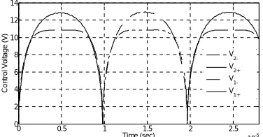
Figure 4 shows control voltage. The electrodes of actuators are located in 100 µm and 200 µm from the base of cantilever, respectively for V1+/V1- and V2+/V

2-(see Figure 1).

As it is shown in Figure 4, the error is in the order of 10-8 which is one hundred times smaller than the desired deflection so the reference signal and the output of the system are overlapped and cannot be distinguished in the figure.

The remained small oscillations are the effect of higher order modes which are truncated from the system model (i.e. the reduced order model) which is used to design controller but included in the plant model. To suppress this unfavorable vibration in the system response one should include more modes in designing the controller.

As explained in controller design section, the pairs of V1+/V1- and V2+/V2- voltages work together to

Figure 2. Estimation error of the tip displacement

Figure 3. Deflection of the tip of the beam and tracking error of the tip for low frequency excitation

Figure 4. Voltages of the Electrodes for tracking control of the beam

5. 3. Tracking with Considering Higher Modes

The effect of the mode contribution in constructing reference signal is investigated by some simulations. Here, we study a reduced model for controller design constructed by three modes. For a model with three modes due to the structure of controller which includes more modes, one should use more control inputs, otherwise the system will not be completely feedback linearizable. This results in using three pairs, i.e. six, of electrodes to produce the control signal in both repelling and attracting directions. The desired reference signal has the following form, and it is desired for tip of the beam to track it.

1 1 2 2 3 3

( ) ( ) (tip) ( ) (tip) ( ) (tip)

r t =r t φ l +r t φ l +r t φ l (27) Simulations just like ones illustrated in Figure 4 are performed to investigate the proper form of the reference signal with respect to frequency of the desired reference signal. The brief results of the simulations are

reported in Table 2. As an example, the frequency of the reference signal is set to be 2.6 MHz which is near the linear natural frequency of the second mode. For comparing different combinations of the reference signal, the RMS value of tracking error and control voltages are listed in Table 2. The configuration that is used in simulations are the same as the preceding one except the number of electrode pairs, which is three here. V1+ and V1- are located at 100 µm from the base of

the beam, V2+ and V2- at 200µm and V3+ and V3- at

300µm, respectively. Plus indexes denote the electrodes that are located below the beam and minus ones denote the above electrodes.

From Table 2, it is clear that choosing appropriate combination of reference signal has crucial effect on the control voltage. In the first raw of the table, the results for the case of r1(t)=1sin(2πvt) µm and r2=r3=0 ,v=2.6

MHz, are depicted. The RMS of tracking error is 2.87e-8 m which is reasonable but the voltages are much higher than the second row which is belongs to the case of r2(t)=1sin(2πvt) and r1=r3=0. In the second case,

since the desired reference signal has frequency near the frequency of the second mode, the tracking performance has been achieved by less control effort which is crucial in MEMS applications. The last case is the most energy consuming case because in which r3(t)=1sin(2πvt) and

r2=r3=0. From these simulations one could conclude that

modes which have the nearest natural frequency to the desired reference signal frequency must have higher contribution in reference signal to avoid excessive control voltage.

5. 4. Comparison of Proposed Model and 1 DOF Model As mentioned in the introduction, some works are dedicated to design controller for one degree of freedom systems. In such systems, the whole body of the beam is modeled by one mass-spring model which significantly simplifies the design efforts. Also, in the case of cantilever beam, one could assume lumped mass and stiffness model and reduce the continuous parameter system into lumped parameter system. Using static deformation to approximate stiffness of the beam causes to overlook effect of higher modes. If the excitation of the beam remains in low frequencies, performance of the controller which is designed based on lumped parameter model will be reasonable. No surprisingly, increasing frequency of the input signal, spoils the output of the system due to model mismatch. Next simulations are dedicated to show the effect of using lumped parameter model to design controller. Two simulations are done to show the significance of modeling method on controller performance. In the first simulation, the frequency of input signal is about the natural frequency of the first mode and in the second one, it is ten time more. In both simulations, the controller is designed by the same method before

0 1 2 3 4 5 6

x 10-6 -0.5

0 0.5 1 1.5 2 2.5 3x 10

-7

Time (sec)

Esti

m

ati

o

n Er

ror

(m)

0 0.5 1 1.5 2 2.5

x 10-5 -2

0 2x 10

-6

Time (sec)

T

ip

D

e

fl

e

c

tio

n

(

m)

0 0.5 1 1.5 2 2.5

x 10-5 -2

0 2x 10

-8

Time (sec)

T

ra

c

k

in

g

Err

o

r

(m)

0 0.5 1 1.5 2 2.5

x 10-5 0

2 4 6 8 10 12 14

Time (sec)

C

o

n

tr

o

l

V

o

lt

a

g

e

(

V)

V 2-V₂₊

V

presented but using equivalent mass and stiffness in one differential equation. The used equation is as follows:

( )

2 2 1

2

eq eq

V

m u k u b

g u

ε

+ =

−

&& (28)

Equivalent mass and stiffness are obtained using Rayleigh method. Parameters are the same as pervious simulations. The original model refers to the model which consists of five modes and developed in pervious sections. The reference signal is a sinusoidal wave with frequency of 250 KHz and amplitude of 1 µm and the second with 2000 KHz and same amplitude. As it is shown in Figure5, using reduced model leads to unfavorable performance of the controller in higher frequencies. The tracking error exceeds the amplitude of input signal due to phase difference between input and output. In low frequency input, as it was predicted, no significant difference occurred.

5. 5. Shape Control Remaining simulations are dedicated to shape control algorithm. The desired shape must satisfy boundary conditions of the beam. For instance cubic function has zero value and zero slopes at the origin which satisfies the boundary conditions of a cantilever beam. It is worthy to mention that making complex shapes with many inflection points needs higher number of actuators and more control effort. In current simulation, the desired shape has the form of a fifth order polynomial like f(x) = Ax5, which satisfies BCs of a cantilever beam and four electrodes, is used. The configuration of electrodes is the same as tracking control simulation in section 5.2. In Figure 6, the desired and actual shape of the beam and error between them are shown. The results show the steady state responses of the system. It is clear that the shape control system forms the beam to the desire shape with little deviation and the largest value of error is seen at the tip of the beam. In Figure 7, required control voltages are depicted. Because the desired shape is static, control voltages approaches to a constant value. Two electrodes (V1+ and V2-) have no contribution in the shape control,

and it is obtained automatically from the controller output.

Figure 5.Tracking error of beam’s tip position using original model and reduced model with reference signal of 250 KHz (top) and 2000 KHZ (bottom).

Figure 6. Desired and actual shape of the beam after control (top) and difference between them (bottom)

Figure 7.Control voltages for shape control

TABLE 1. Parameters of the simulated microbeam and displacement sensor

Beam length (µm) Thickness (µm) width (µm) Initial gap (µm) Effective Young’s modulus (GPa) Density

300 3 20 2 160 2500

Nominal measurement range (µm)

Static resolution (% of measurement Range)

Dynamic resolution (% of measurement Range)

Linearity (% of measurement Range)

20 0.001 0.002 3

TABLE 2. RMS values of tracking error and control voltages for different combinations of reference signal

Mode Contribution amplitude ofr1 r2 r3 Tracking Error(m) V₁₊(V) V_1-(V) V₂₊(V) V_2-(V) V₃₊(V) V_3-(V)

[1µm 0 0] _{2.8708e-008 116.2 115.1 192.2 191.5 270.8 263.6}

[0 1µm 0] _{2.5230e-008 73.7 58.9 65.0 51.9 50.1 61.8}

[0 0 1µm] _{1.8621e-008 330.5 338.9 335.0 326.5 249.2 245.3}

0 0.5 1 1.5 2 2.5

x 10-5

-1 0 1

2x 10

-7

Time (sec)

T

ra

c

k

ing

E

rr

o

r

(m)

0 0.5 1 1.5 2 2.5

x 10-5

-2 0

2x 10

-6

Time (sec)

T

ra

c

k

in

g

E

rr

o

r

(m)

Original Model Reduced Model

Original Model Reduced Model

0 1 2 3

x 10-4 -1

0 1 2x 10

-6

Beam Length (m)

F

in

al

S

h

a

pe

(

m)

0 1 2 3

x 10-4 -4

-2 0 2x 10

-7

Beam Length (m)

S

hape

Err

o

r

(m)

Actual Shape Desired Shape

0 0.5 1 1.5 2 2.5 3 3.5 4 4.5 5

x 10-5

0 50 100 150 200 250

Time (sec)

C

on

tr

o

l

V

o

lt

ag

e

(

V)

V₁₊

V₂₊

V

2-5. CONCLUSION

In this research, the partial differential equation of motion of an electrostatically actuated micro-cantilever has been approximated by a set of nonlinear ordinary differential equations using Galerkin projection method. The ODEs are coupled because of nonlinearity in PDE. Observabillity of a model that consists of two modes have been proved and an estimation system based on the EKF method is designed. Then, a tracking control system is designed by feedback linearization method. By this controller selected points of the beam track reference signals. The relation of modes included in the model and frequency of the reference signal and its effect on the performance of the system are investigated. Simulation results show that the modes which are chosen to be used in model must be matched with the frequency of tracking signal. Based on the designed tracking control algorithm, a shape control algorithm is proposed that forms the beam into a desired shape.

6. REFERENCES

1. Younis, M.I., "Mems linear and nonlinear statics and dynamics:

Mems linear and nonlinear statics and dynamics, Springer, Vol. 20, (2011)

2. Seok, J. and Scarton, H.A., "Dynamic characteristics of a beam angular-rate sensor", International Journal of Mechanical Sciences, Vol. 48, No. 1, (2006), 11-20.

3. Kamisuki, S., Fujii, M., Takekoshi, T., Tezuka, C. and Atobe, M., "A high resolution, electrostatically-driven commercial inkjet head", in Micro Electro Mechanical Systems,. MEMS. The Thirteenth Annual International Conference on, IEEE. (2000), 793-798.

4. Chu, L.L., Que, L. and Gianchandani, Y.B., "Measurements of material properties using differential capacitive strain sensors",

Microelectromechanical Systems, Journal of ,Vol. 11, No. 5, (2002), 489-498.

5. Hassanpour, P.A., Nieva, P.M. and Khajepour, A., "Stochastic analysis of a novel force sensor based on bifurcation of a micro-structure", Journal of Sound and Vibration, Vol. 330, No. 23, (2011), 5753-5768.

6. Yasuda, T., Shimoyama, I. and Miura, H., "Electrostatically driven micro elastic joints", in Intelligent Robots and Systems 95.'Human Robot Interaction and Cooperative Robots', Proceedings. IEEE/RSJ International Conference on, IEEE. Vol. 2, (1995), 241-252.

7. Chau, H.L. and Wise, K.D., "An ultra miniature solid-state pressure sensor for a cardiovascular catheter", IEEE Transactions on Electron Devices, Vol. 35, (1988), 2355-2362. 8. Ganji, B. and Nateri, M.S., "Modeling of capacitance and sensitivity of a mems pressure sensor", International Journal of Engineering-Transactions B: Applications, Vol. 26, No. 11, (2013), 1331-1340.

9. Abdel-Rahman, E.M., Younis, M.I. and Nayfeh, A.H., "Characterization of the mechanical behavior of an electrically actuated microbeam", Journal of Micromechanics and Microengineering, Vol. 12, No. 6, (2002), 759-770.

10. Brusa, E., DeBona, F., Gugliotta, A. and Soma, A., "Modeling and prediction of the dynamic behaviour of microbeamsunder electrostatic load", AnalogIntegrated Circuits and Signal Processing, Vol. 40, No. 2, (2004), 155-164.

11. Batra, R.C., Porfiri, M. and Spinello, D., "Electromechanical model of electrically actuated narrow microbeams",

Microelectromechanical Systems, Journal of, Vol. 15, No. 5,(2006), 1175-1189

12. Mojahedi, M., Moghimi Zand, M. and Ahmadian, M., "Static pull-in analysis of electrostatically actuated microbeams using homotopy perturbation method", Applied Mathematical Modelling, Vol. 34, No. 4, (2010), 1032-1041.

13. Abbasnejad, B., Shabani, R. and Rezazadeh, G., "Stability analysis in parametrically excited electrostatic torsional micro-actuators", International Journal of Engineering-Transactions C: Aspects, Vol. 27, No. 3, (2013), 487.

14. Rezazadeh, G., Tahmasebi, A. and Ziaei-rad, S., "Nonlinear electrostatic behavior for two elastic parallel fixed–fixed and cantilever microbeams", Mechatronics, Vol. 19, No. 6, (2009), 840-846.

15. Ganji, B.A. and Mousavi, A., "Accurate determination of pull-in voltage for mems capacitive devices withclamped square diaphragm", International Journal of Engineering Transactions B: Applications, Vol. 25, No. 3, (2012), 161-166. 16. Lakrad, F. and Belhaq, M., "Suppression of pull-in instability in

mems using a high-frequency actuation " ,Communications in Nonlinear Science and Numerical Simulation, Vol. 15, No. 11, (2010), 3640-3646.

17. Wang, P., "Feedback control of vibrations in a micromachined cantilever beam with electrostatic actuators", Journal of Sound and Vibration, Vol. 213, No. 3, (1998), 537-550.

18. Kharrat, C., Colinet, E. and Voda, A., "Microbeam dynamic shaping by closed-loop electrostatic actuation using modal control", in Research in Microelectronics and Electronics Conference,. PRIME (2007), 197-205

19. Kharrat, C., Colinet, E. and Voda, A., "A robust control method for electrostatic microbeam dynamic shaping with capacitive detection", in Proceedings of the 17th World Congress, The International Federation of Automatic Control. (2008), 568-573. 20. Vagia, M., Nikolakopoulos, G. and Tzes, A., "Design of a

robust pid-control switching scheme for an electrostatic micro-actuator", Control Engineering Practice, Vol. 16, No. 11, (2008), 1321-1328.

21. Vagia, M., "A frequency independent approximation and a sliding mode control scheme for a system of a micro-cantilever beam", ISA Transactions, Vol. 51, No. 2, (2012), 325-332. 22. Kucuk, I., Sadek, I.S., Zeini, E. and Adali, S., "Optimal vibration

control of piezolaminated smart beams by the maximum principle", Computers & Structures, Vol. 89, No. 9, (2011), 744-749.

23. ٢Hu, F., Yao, J., Qiu, C. and Ren, H., "A mems micromirror driven by electrostatic force", Journal of Electrostatics, Vol. 68, No. 3, (2010), 237-242.

24. Bonora, S., "Distributed actuators deformable mirror for adaptive optics", Optics Communications, Vol. 284, No. 13, (2011), 3467-3473.

25. Cugat, O., Basrour, S., Divoux, C., Mounaix, P. and Reyne, G., "Deformable magnetic mirror for adaptive optics :Technological aspects", Sensors and Actuators A: Physical, Vol. 89, No. 1, (2001), 1-9.

26. Vatankhah, R., Karami, F., Salarieh, H., Alasty, A. and "Stabilization of a vibrating non-classical micro-cantilever using electrostatic actuation", ScientiaIranica: Transaction on Mechanical Engineering, Vol. 20, No. 6, (2013), 1824- 1831.

APPENDIX A

2 2 2 2 2 2

0 1 2 2 1 2 0 2 1 1 1 1 2 1 2 1 1

2 2 2 2 2 2 2 2

3 1 2 2 2 1 32 2 4 1 1 2 4 2 1 2

2 2 2 2

2 3 1 2 2 1 4 1 1 3 2 2 4 2 1

2 2 2 2 2 2 2

2 1 4 1 2 1 1 3 2 0 2

2 2 1

(2 2 )

( )

V a y y V b V a y V b y V a y V a y V b y V b y V a y y V b y y P V a y V a y V b y V b y

a V y a V y y a V y a V y a y P

V V y

φ φ φ φ φ φ φ

φ φ φ φ φ

φ φ φ φ φ φ

− − + + + +

+ + + +

= − − + + +

+ + + + − +

= +

1 1 12 2 1 1 4 1 2 2 2 1 4 2 2 (aφ+bφ +2aφy +aφy +2bφy +bφy)

2 2 2 2 2 2

1 1 1 2 2 1 1 4 1 2 2 2 1 4 2 2

2 2 2 2

3 1 2 2 1 4 1 1 3 2 2 4 2 1

2 2 2 2 2 2

3 1 2 1 4 2 3 1 2 2 1 4 1 1 3 2 2

2 2 2 2 2 2

4 2 1 4 1 4 2 2 1 4 1

2

2 2

2 2

( 2 ) (2 2

) ( )(

V a V b V a y V a y V b y V b y

V a y V a y V b y V b y

Q V a V a y V a y V a y V a y V b y

V b y V a V b a V y a V Q

Q

y

φ φ φ φ φ φ

φ φ φ φ φ φ

φ φ φ φ φ

φ φ φ

+ + + + + − − + + + = + + + − − + + + + = + = + 2

1 2 1 1

2 2 2 2

3 2 0 2 2 2 1 2 2

2 2 2 2

4 3 2 4 1 3 1 2 2 1 4 1 1

2 2 2 2

3 2 2 4 2 1 3 1 3 2

2 2 2 2 2 2 2

2 1 4 1 2 1 1 3 2 0 2 2

1 1 1 2 2 1 1 4 1 2

) (2 2 )

(2 1 )(2

2 ) (2 2 )

( )

( 2 2

y a V y

a V y a V y V y a b

Q V a y V a y V a y V a y

V b y V b y V a V b

a V y a V y y a V y a V y a V y

V a b a y a y

φ φ

φ φ φ φ

φ φ φ φ

φ φ φ φ

+ + + − + + = − + − − + + + + + + + + + + + + + + − 2

2 2 1 4 2 2) 2(4 1 4 2) bφy+bφy +V y aφ+bφ

APPENDIX B

ij

a and bij are the same for the proposed observer and

controller systems. ( ) ( ) ( ) ( ) ( ) ( ) ( ) ( ) ( ) ( ) ( ) ( ) ( ) ( ) ( ) ( ) ( ) ( ) ( ) ( ) ( ) ( ) ( ) ( ) ( ) 1 1

0 ₀ 1 1 ₀ 1 1

1 1

2 2

2 ₀ 1 1 3 ₀ 1 2

1 1

4 ₀ 1 1 2 0 ₀ 2

1 1

2

1 ₀ 2 1 2 ₀ 2 1

3 ₀ 2

, 2

3 , 3

6 ,

2 , 3

3

x x

i _x i i _x i

x x

i _x i i _x i

x x

i _x i i _x i

x x

i _x i i _x i

i _x i

a x x dx a x x x dx

a x x x dx a x x x dx

a x x x x dx b x x dx

b x x x dx b x x x dx

b x x

φ ψ φ ψ φ

φ ψ φ φ ψ φ

φ ψ φ φ φ ψ

φ ψ φ φ ψ φ

φ ψ = = = = = = = = = = = = = = = = = = = = = = = = = = ∫ ∫ ∫ ∫ ∫ ∫ ∫ ∫ ( ) ( ) ( ) ( ) ( ) 1 1 2

2 , 4 ₀6 2 1 2

x x

i _x i

x dx b x x x x dx

φ φ ψ φ φ

= =

=

=

∫ ∫

2 2

11 10 11 1 12 1 13 2 14 1 2

2 2

12 10 11 1 12 1 13 2 14 1 2

2 2

21 20 21 1 22 1 23 2 24 1 2

2 2

22 20 21 1 22 1 23 2 24 1 2 P a a u a u a u a u u

P b b u b u b u b u u

P a a u a u a u a u u

P b b u b u b u b u u

= + + + + = + + + + = + + + + = + + + + APPENDIX C 2 14 1 13 3 2

1 1 1 2 1 14 3

2 21 2 4 1 2 3 3 2

2 2 1 2 4 3 1 1

2 1

( ) ˆ ,

0

0 1 0

ˆ ˆ

( 2 )

ˆ ˆ

1 ( 2 ) 0 0

0

0 0 1

ˆ ˆ

1 ( 2 )

ˆ ˆ

( 2 ) 0 0

( ) 0 0 0

0 0 0 0

( )

ˆ , 0 0 ( ) 0

0 0 0 0

f F t

x V x

a x a x V a a x a x V

a a x a x V a x a x V

l h

H t

x V l

x φ φ ∂ =_∂ =   ₊  _{− + + +}      − + + +  ₊         ∂ _{ } =_{∂ =  }    

Tracking and Shape Control of a Micro-cantilever using Electrostatic Actuation

F. Karamia_{, H. Salarieh} a_{, R. Shabani}b

a _{Department of Mechanical Engineering, Sharif University of Technology, Tehran, Iran} b_{Department of Mechanical Engineering, Faculty of Engineering, Urmia University, Urmia, Iran}

P A P E R I N F O

Paper history:

Received 02 November 2013 Received in revised form 14 May 2014 Accepted 22 May 2014

Keywords: Micro-cantilever Electrostatic Actuation State Estimation Tracking Control Shape Control هﺪﯿﮑﭼ

ﯽﻄﺧﺮﯿﻏﮏﯾﺮﺤﺗﺎﺑﺮﯿﮔردﺮﺴﮑﯾﺮﯿﺗوﺮﮑﯿﻣﮏﯾﻞﮑﺷلﺮﺘﻨﮐويﺮﯿﮕﻫرلﺮﺘﻨﮐ،ﺖﻟﺎﺣيﺎﻫﺮﯿﻐﺘﻣﻦﯿﻤﺨﺗﻪﻟﺄﺴﻣﻪﻟﺎﻘﻣﻦﯾارد

ﺖﺳا ﻪﺘﻓﺮﮔراﺮﻗﯽﺳرﺮﺑ درﻮﻣﯽﮑﯿﺗﺎﺘﺳاوﺮﺘﮑﻟا

.

هرﺎﭘ ﻞﯿﺴﻧاﺮﻔﯾدتﻻدﺎﻌﻣرﻮﻈﻨﻣ ﻦﯾاياﺮﺑ

شورزا هدﺎﻔﺘﺳاﺎﺑ ﻢﺘﺴﯿﺳيا

ﻦﯿﮐﺮﻟﺎﮔ

ﺖﺳاهﺪﺷﻞﯾﺪﺒﺗﯽﻟﻮﻤﻌﻣﻞﯿﺴﻧاﺮﻔﯾدتﻻدﺎﻌﻣزاﺖﺳﮏﯾﻪﺑ

.

هﺪﻫﺎﺸﻣتﺎﺒﺛازاﺲﭘ

ﻢﺘﯾرﻮﮕﻟاﮏﯾﻢﺘﺴﯿﺳيﺮﯾﺬﭘ

رد،هﺪﺷهدزﻦﯿﻤﺨﺗيﺎﻫﺮﯿﻐﺘﻣزاوهﺪﺷﯽﺣاﺮﻃﻪﺘﻓﺎﯾﻪﻌﺳﻮﺗﺮﺘﻠﯿﻓﻦﻤﻟﺎﮐشورسﺎﺳاﺮﺑنآياﺮﺑﺖﻟﺎﺣيﺎﻫﺮﯿﻐﺘﻣﻦﯿﻤﺨﺗ

ﺖﺳاهﺪﺷهدﺎﻔﺘﺳاﺚﺤﺑدرﻮﻣلﺮﺘﻨﮐﻢﺘﺴﯿﺳ

.

ﻨﻣﻪﺑلﺮﺘﻨﮐﻢﺘﺴﯿﺳ

هﺪﺷﯽﺣاﺮﻃﺮﯿﺗزاﺮﻈﻧدرﻮﻣطﺎﻘﻧﺖﮐﺮﺣﺮﯿﺴﻣلﺮﺘﻨﮐرﻮﻈ

ﺖﻓﺮﮔراﺮﻗﯽﺳرﺮﺑدرﻮﻣهﺪﻨﻨﮐلﺮﺘﻨﮐﻦﯾايورﺮﺑلﺮﺘﻨﮐياﺮﺑﺐﺨﺘﻨﻣيﺎﻫدﻮﻣﺮﺛاو

.

لﺮﺘﻨﮐزاهدﺎﻔﺘﺳاﺎﺑنﺎﯾﺎﭘرد ﺮﯿﺴﻣهﺪﻨﻨﮐ

ﺪﯾدﺮﮔدﺎﻬﻨﺸﯿﭘﺮﯿﺗياﺮﺑﻞﮑﺷلﺮﺘﻨﮐﻢﺘﯾرﻮﮕﻟاﮏﯾ،هﺪﺷﯽﺣاﺮﻃ

.

ﻢﺘﯾرﻮﮕﻟاﻦﯾاﻪﻋﻮﻤﺠﻣ

هدﺎﻔﺘﺳاﺎﺑﺎﻫ ﻪﯿﺒﺷزا

يدﺪﻋيزﺎﺳ

ﻪﺤﺻ

ﻪﺘﻓﺮﮔراﺮﻗﺚﺤﺑدرﻮﻣﺞﯾﺎﺘﻧوهﺪﺷيراﺬﮔ

ﺪﻧا

.

doi:10.5829/idosi.ije.2014.27.09c.14