The Efficiency of MSBM Model with Imprecise Data (Interval)

343

Vol.2, No.1, Year 2014 Article ID IJDEA-00216, 8 pages Research Article

The Efficiency of MSBM Model with

Imprecise Data (Interval)

F. seyed Esmaeili a*

(a) Department of Mathematics, Islamic Azad University, South Tehran Branch, Tehran, Iran

Received 18 January 2014, Revised 27 February 2014, Accepted 15 March 2014

Abstract

Data Envelopment Analysis (DEA) is a mathematical programming-based approach for evaluates the relative efficiency of a set of DMUs (Decision Making Units). The relative efficiency of a DMU is the result of comparing the inputs and outputs of the DMU and those of other DMUs in the PPS (Production Possibility Set). Also, in Data Envelopment Analysis various models have been developed in order to evaluate the performance of decision-making units with negative data. The Modified Slack Based Measure (MSBM) model is from collective models family. This modified model is based on slack-based measure (SBM). Also the early models of data envelope analysis considered inputs and outputs as precise data. However, in studies about the data envelope analysis, some methods presented for applying imprecise data. Based on this, data envelope analysis models with interval data have been developed. In this paper, the MSBM model is investigated in presence of interval negative data, and then the efficiency of the model with imprecise data (interval) is evaluated. The efficiency of ten decision-making units is evaluated.

Keywords: Data envelopment analysis, modified model, interval data, evaluating the efficiency of negative data.

1. Introduction

Data Envelopment Analysis (DEA) is a non-parametric technique for measuring and evaluating the relative efficiency of a set of Decision Making Units (DMU) with alternative inputs and outputs. The DEA was firstly proposed by Charnes, Cooper, and Rhodes [2] in the well-known paper CCR, and further continued in literature by others like Banker [1]. In all original models of DEA, the default assumption is that all input/output values are positive. This strict constraint first applied by Charnes et al. on CCR model in 1987, and then by other scientists on other models. However, in practical problems, there are many cases where this constrained is violated, and there exist negative inputs and outputs. In

* _{Corresponding author:}

F. seyed Esmaeili,et al /IJDEA Vol.2, No.1, (2014). 343-350 433

aspect of theoretical and practical development of DEA, in recent years many researchers have focused on issue of DEA with negative data. The works of Seiford and Zhu [4] are among the most important methods presented. Another useful method belongs to Silva Portela [6] in RDM paper. Another method, which so far has had the greatest share of dealing with negative data, is the method developed by Sharp [5] named MSBM. Sharp made this model applicable to negative data by modifying SBM model. Emrooznejad [3] obtained an acceptable efficiency measure by this method with precise data.

In recent years imprecise data is important, because in many real problems decision maker encounters risk and uncertainty conditions where it is not possible to determine precise and reliable values for each input or output. To overcome this shortcoming, Wang [7] proposed the pattern of Interval Data Envelop Analysis (IDEA) i.e. a case of imprecise data. Applying some theoretical changes to data envelop analysis models, such data can be used and the results from efficiency evaluation can be obtained.

method, then the model is presented with imprecise data. Furthermore, the efficiency of ten DMUs is evaluated by applying the presented model.

2. A review on the method of Modified Slack Based Measure (M.S.B.M)

Sharp et al. made a balance in order to calculate the efficiency measure in presence of negative variables by using the Portela method and substituting enhancement vectors (R_io,R_ro) with observation values in the target function of SBM model so that it would be applicable for negative data. This model is known as MSBM as follow:

p̃ = min 𝑜

1 − ∑ w𝑖s𝑖

− 𝑅𝑖𝑜 m i=1

1 + ∑ v𝑟s𝑟

+ 𝑅𝑟𝑜 s r=1

S. t ∑ λj n

j=1

x̃ + sij i−= x̃ , i = 1, … , m io

∑ λj n

j=1

ỹ − srj r+= ỹ , r = 1, … , s (1) ro

∑ λj n

j=1

= 1

λj≥ , s𝑖−≥ 0, sr+≥ 0 , j = 1, … , n , r = 1, … , s , i = 1, … , m where:

s_i−: the value of ith input slack

s_r+: the value of ith output slack

In addition, vectors in the model are as below:

Rro= Max_j {yrj} − yro , Rio = xio− Min_j {xij}

When R_io and R_ro are equal to zero, it is assumed that WiSi−

Rio and

VrSr+

Rro terms are eliminated from

nominator and denominator. The efficiency measure of MSBM falls in the interval of [0 , 1]. Furthermore, the model is not only unit stable but also shift stable too, and is applicable with negative data.

2.1. The efficiency of MSBM model with imprecise data (interval)

The classic models of data envelop analysis are used for measuring the efficiency of units with precise data. However, since in real world decision-making is accompanied with uncertainty conditions and imprecise information, precise values cannot be determined for data. This questions the precision and accuracy of measurements. The method of interval data envelope analysis takes advantage of new applicable techniques for measuring efficiency in case of uncertainty. In IDEA model, the value of each input and output falls in an interval and can be variable in that interval too. If each of the n units uses m different units for producing s

outputs, then DMU_j , j =

1

, … , n makes use of X_j = [x_1j, x_2j, … , x_mj]t _{i =}

1

_{, … , m inputs to}

output Y_j= [y_1s, y_2s, … , y_sj]t_{،r =}

1

_{, … , s. These inputs and outputs are not precisely available}

only their lower and upper bounds are available as follow:

𝑦_𝑟𝑗 ∈ [𝑦_𝑟𝑗𝑙 , 𝑦_𝑟𝑗𝑢] , 𝑥_𝑖𝑗 ∈ [𝑥_𝑖𝑗𝑙 , 𝑥_𝑖𝑗𝑢]

x_ijl and y_rjl are lower bounds, and x_iju and y_rju are upper bounds for inputs and outputs.

Table1.Input and output structure for interval data envelopment analysis model

In the following, two models are proposed so that the optimum values of their target functions

give the lower and upper bounds of the optimum value of the target function of model (

1

). This

will be proven in theorem

1

.

DMU 𝑋1 … 𝑋𝑚 𝑌1 … 𝑌𝑚

𝐷𝑀𝑈₁ [𝑥₁₁𝑙 , 𝑥₁₁𝑢 ] … [𝑥_1𝑚𝑙 _{, 𝑥}

1𝑚𝑢 ] [𝑦11𝑙 , 𝑦11𝑢] … [𝑦1𝑚𝑙 , 𝑦1𝑚𝑢 ]

𝐷𝑀𝑈₂ [𝑥₂₁𝑙 , 𝑥₂₁𝑢 ] … [𝑥_2𝑚𝑙 , 𝑥_2𝑚𝑢 ] [𝑦₂₁𝑙 , 𝑦₂₁𝑢 ] … [𝑦_2𝑚𝑙 , 𝑦_2𝑚𝑢 ]

. . . . .

. . . . .

. . . . .

𝐷𝑀𝑈_𝑛 [𝑥_𝑛1𝑙 _{, 𝑥}

F. seyed Esmaeili,et al /IJDEA Vol.2, No.1, (2014). 343-350 433

Model (

2

) shows a lower bound of unit efficiency J_o interval:

p𝑜𝐿 = min

1 − ∑ wisi

−

R𝑖𝑜

m i=1

1 + ∑ vrsr+

R_𝑟𝑜

s r=1

S. t ∑ λ_j

n

j=1

x_ijL+ s_i− = x_iou , i = 1, … , m

∑ λj

n

j=1

Y_rju− sr+ = yroL , r = 1, … , s (2)

∑ λ_j

n

j=1

= 1

λ_j ≥ 0 , s_𝑖− ≥ 0 , s_r+ ≥ 0 , j = 1, … , n , r = 1, … , s , i = 1, … , m

Rro = yrMaxu− yiMinl and Rio= xrMaxu− xiMinl

Model (

3

) shows an upper bound of unit efficiency J_o interval:

p_𝑜𝑢 _{= min}

1

− ∑ wisi−

R_𝑖𝑜

m i=1

1

+ ∑ v_Rrsr+

𝑟𝑜 s r=1

S. t ∑ λj

n

j=1

x_iju+ s_i− = x_iol , i = 1, … , m

∑ λ_j

n

j=1

Y_rjl − s_r+ _{= y}

rou , r = 1, … , s (3)

∑ λj

n

j=1

= 1

λj ≥ 0 , s𝑖− ≥ 0 , sr+ ≥ 0 , j = 1, … , n , r = 1, … , s , i = 1, … , m

In model 3, DMU is in the best case for evaluation and pps boundary is in the worst case. On

the other hand, in model

2

, DMU is in the worst case for evaluation and pps boundary is in

the best case. Now, it is illustrated in the following theorem that P̃ ∈ [P_{o o}l_{, P}

ou]. Theorem

1

: if P_oU_{, P}

oL, and P̃o are the optimums of target functions of models (

1

), (

2

), (

3

)

respectively, then: P_oL ≤ P̃ ≤ P_{o o}U

Proof: assume that λ̃ and s̃ is the optimum of model (

1

). ∑𝑛_𝑗=1𝜆̃_𝑗x_𝑖𝑗𝑙 ≤ ∑𝑛_𝑗=1𝜆̃_𝑗x_𝑖𝑗𝑙 + λ̃x_{𝑜 𝑖𝑜}𝑢

Since, ∑𝑛_𝑗=1𝜆̃𝑗x𝑖𝑗𝑙 +̃xλ𝑜 𝑖𝑜𝑢 = 𝑥𝑖𝑜𝑢 − 𝑠̃𝑖−, therefore we have:

∑

𝑛𝑗=1𝜆

̃

𝑗xijl + 𝑠

̃

𝑖− ≤ x𝑖𝑜𝑢

Now, ∃ ŝ ≥ si− ̃i− thus we have:

∑

𝑗=𝑛 1𝜆

̃

𝑗xijl + s

̂

i− = x𝑖𝑜𝑢

Now, for output variables we have: ∑𝑛_𝑗=1𝜆̃_𝑗y_𝑟𝑗𝑢 ≥ ∑𝑛_𝑗=1𝜆̃_𝑗y_𝑟𝑗𝑢 + λ̃y_{𝑜 𝑟𝑜}𝑙

Since, ∑𝑛_𝑗=1𝜆̃_𝑗y_𝑟𝑗𝑢 +λ̃y_{𝑜 𝑟𝑜}𝑙 _{= y}

𝑟𝑜𝑙 + 𝑠̃𝑟+, therefore we have:

∑

𝑛𝑗=1𝜆

̃

𝑗y𝑟𝑗

𝑢 _{− 𝑠}

𝑟 +

̃

_{≥ y}

𝑟𝑜 𝑙

Now, ∃ ŝ ≥ s_r+ ̃_r+, thus we have:

∑

_𝑗=𝑛 ₁𝜆

̃

_𝑗y_𝑟𝑗𝑢 − s

̂

_r+ _{= y} 𝑟𝑜 𝑙

The value of its target function is as below:

Since

s_{̂ ≥ s𝑖}− 𝑖 −

̃ so ∑ w𝑖ŝ𝑖−

𝑅𝑖𝑜

m

i=1 ≥ ∑

w𝑖s̃𝑖−

𝑅𝑖𝑜

m

i=1 then 1 − ∑

w𝑖ŝ𝑖−

𝑅𝑖𝑜

m

i=1 ≤ 1 − ∑

w𝑖s̃𝑖−

𝑅𝑖𝑜

m

i=1 (4)

Since

ŝ ≥ s_𝑟+ ̃ so 1 + ∑_𝑟+ vrsr

+

̂

R_𝑟𝑜

s

r=1

≥ 1 + ∑vrsr

+

̃

R_𝑟𝑜

s

r=1

then 1

1 + ∑ v_Rrŝr+

𝑟𝑜 s r=1

≤ 1

1 + ∑ vrs̃r+

R_𝑟𝑜

s r=1

(5)

(4)و(5) we have

1 − ∑ w_𝑅𝑖ŝ𝑖−

𝑖𝑜 m i=1

1 + ∑ v_Rrŝr+

𝑟𝑜 s r=1

≤

1 − ∑ w_𝑅𝑖s̃𝑖−

𝑖𝑜 m i=1

1 + ∑ vrs̃r+

R_𝑟𝑜

s r=1

= 𝑝̃

Regarding that s̃ and λ̃ _{is a feasible solution of minimization problem (}

1

_{), therefore the}

optimum of target function of model (

2

) equals to p𝑙, and is smaller or equal to the value of

F. seyed Esmaeili,et al /IJDEA Vol.2, No.1, (2014). 343-350 433

In other words, p𝑙 _{≤ p̃}

.

Similarly, it is proven that p𝑢 ≥ p̃.

Now, with respect to the proven theorem, an efficiency interval can be obtained for each of the

decision making units by solving the two nonlinear programming models (

2

) and (

3

).

In order to determine and measure the efficiency of each decision-making unit, the following

sets are introduced:

E++_{= { j ∈ J | P}

jL= 1 }

E+ _{= { j ∈ J │ P}

jL < 1 , PjU = 1}

E− = { j ∈ J │ P_jU < 1 }

In the above sets, if P_jL= 1, then the jth _{decision-making unit is efficient for all values of}

input/output intervals. However, if P_jL< 1 and P_jU = 1, the jth decision-making unit is only

efficient for the upper bounds of input/output intervals. If P_jU < 1, the jth _{decision-making unit}

is not efficient for any values in the input/output intervals.

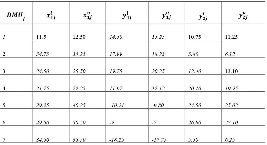
3. A numerical example

Assume that there are ten DMUs with one input and two outputs intervals according to the

table below.

Table 2: Ten DMU with one input and two outputs

𝒚𝟐𝒋𝒖 𝒚_𝟐𝒋𝒍

𝒚𝟏𝒋𝒖 𝒚𝟏𝒋𝒍

𝒙𝟏𝒋𝒖 𝒙𝟏𝒋𝒍

𝑼𝑴𝑫_𝑱

22.11

27.01

15.25

14.50

21.17

22.1

1

6.12

5.80

18.23

17.99

35.25

34.75

1

21.27

12.40

20.25

19.75

25.50

24.50

1

19.95

20.10

12.12

11.97

22.25

21.75

4

25.02

24.50

-9.80

-10.21

40.25

39.25

1

27.10

26.80

-7

-9

50.50

49.50

6

6.25

5.50

-17.75

-18.25

35.50

34.50

In table

2

, inputs and outputs are given in form of intervals for each DMU. For more

investigation, the MSBM model with interval data in table

2

is ran by GAMS software. The

upper and the lower bounds of efficiency are investigated, and the efficiency of each unit is

presented in table

3

.

Furthermore, the model

2

and

3

are solved by software assigning the weight of

0.50

for each v_r

and the weight of

1

for each w_i.

Table

3

: Efficiency results for interval data

In the table above, for DMUs that are located in the best conditions outside PPS and become

super-efficient, the efficiency value is shown with 1+. Thus, as it is observed in the above table,

according to the obtained results, DMU₁ , DMU₃ , DMU₄, DMU₅ , DMU₆ , DMU₁₀ are efficient

in their owns best condition and DMU₂, DMU₇ , DMU₈, DMU₉ given that the upper bound of

their efficiency is smaller than

1

, are inefficient and also all DMUs are inefficient in their own

22.06

21.99

-9.50

-10.50

40.21

39.99

8

19.05

18.75

-6

-8

25.25

24.75

9

8.19

7.75

26.50

25.50

2

6.50

15.50

27

p_𝑗𝑢 p_𝑗𝑙

𝐷𝑀𝑈_𝑗

1+

7.911

2

7.418

7.101

1

1+

7.007

1

1+

7.991

4

1+

7.809

1

1+

7.926

6

7.198

7.111

0

7.646

7.621

8

7.014

7.022

9

1+

F. seyed Esmaeili,et al /IJDEA Vol.2, No.1, (2014). 343-350 453

worst conditions; among which DMU₄ and DMU₇have respectively maximum and minimum

efficiency in their own the worst conditions and thus we have following category for DMUs:

E+ = {DMU1 , DMU3 , DMU4, DMU5 , DMU6 , DMU10}،

E− = {DMU2 , DMU7 , DMU8, DMU9} and E++= ∅

4. Conclusion

The MSBM model, introduced by Sharp [5] i.e. among the most powerful proposed models for evaluating units with negative data, was extended in form of interval. Therewith, two models with lower and upper bounds target function were obtained. It was also proven that the optimum of lower bound was less than or equal to the optimum of upper bound. Furthermore, ten DMUs were evaluated in term of efficiency with respect to the obtained models in the studied example, 7 out of 10 units were only in the upper bound and 3 units were always inefficient and no DMU become efficient in its own worst conditions.

References

[

1

] Banker. R. Charnes. A.Cooper. W.W.

1984

. Some models for estimating technical and scale

ineciencies in data envelopment analysis. European. Journal of Operational Research

30(9) .

1078-1092

.

[

2

] Charnes A, Cooper WW, Rhodes E., Measuring the efficiency of decision making units,

European Journal of Operational Research;

2:429- 440, (1978).

[

3

] Emrouznejad, A., Anouze, A. L., & Thanassoulis, E. (

1727

).A semi-oriented radial measure

for measuring the efficiencies of decision making units with negative data, using

DEA.European Journal of Operational Research,

177,190-174

.

[

4

] Seiford LM and Zhu J (

2002

) .Modeling undesirable factors in efficiency evaluation. Eur J

Opl

142 : 16-20

[

5

] Sharp, J. A., Meng, W., & Liu, W. (

2006

). A modified slacks-based measure model for data

envelopment analysis with ‘natural’ negative outputs and inputs. Journal of the Operational

Research Society,

58, 1672

–

1677

.

[

6

] Silva Portela, M. C. A., Thanassoulis, E., & Simpson, G. (

1774

). Negative data in DEA: A

directional distance approach applied to bank branches. Journal of the Operational Research

Society,

11, 2222

–

2212

.

[

7

] Wang, Y.M., Great banks, R.& Yang, B. (

2005

) Interval Efficiency Assessment Using Data