University of Warwick institutional repository: http://go.warwick.ac.uk/wrap
This paper is made available online in accordance with
publisher policies. Please scroll down to view the document
itself. Please refer to the repository record for this item and our
policy information available from the repository home page for
further information.
To see the final version of this paper please visit the publisher’s website.
Access to the published version may require a subscription.
Author(s): P. J. THOMAS and P. F. LINDEN
Article Title: Rotating gravity currents: small-scale and large-scale
laboratory experiments and a geostrophic model
Year of publication: 2007
Link to published version: http://dx.doi.org/
10.1017/S0022112007004739
doi:10.1017/S0022112007004739 Printed in the United Kingdom
Rotating gravity currents: small-scale and
large-scale laboratory experiments and a
geostrophic model
P. J. T H O M A S1A N D P. F. L I N D E N2
1Fluid Dynamics Research Centre, School of Engineering, University of Warwick,
Coventry, CV4 7AL, UK
2Department of Mechanical and Aerospace Engineering, University of California, San Diego,
9500 Gilman Drive, La Jolla, CA 92093-0411, USA
(Received14 December 2005 and in revised form 31 October 2006)
Laboratory experiments simulating gravity-driven coastal surface currents produced by estuarine fresh-water discharges into the ocean are discussed. The currents are generated inside a rotating tank filled with salt water by the continuous release of buoyant fresh water from a small source at the fluid surface. The height, the width and the length of the currents are studied as a function of the background rotation rate, the volumetric discharge rate and the density difference at the source. Two complementary experimental data sets are discussed and compared with each other. One set of experiments was carried out in a tank of diameter 1 m on a small-scale rotating turntable. The second set of experiments was conducted at the large-scale Coriolis Facility (LEGI, Grenoble) which has a tank of diameter 13 m. A simple geostrophic model predicting the current height, width and propagation velocity is developed. The experiments and the model are compared with each other in terms of a set of non-dimensional parameters identified in the theoretical analysis of the problem. These parameters enable the corresponding data of the large-scale and the small-scale experiments to be collapsed onto a single line. Good agreement between the model and the experiments is found.
1. Introduction
When estuarine water is discharged into the coastal zone, gravity-driven surface flows can be established. These flows develop as a consequence of the density difference between the buoyant estuarine fresh water and the denser, salty ocean water. For sufficiently large discharge rates, i.e. when the current exceeds length scales larger than the Rossby deformation scale, the current dynamics are affected by the Coriolis force arising from the rotation of the earth. As a result the discharged fresh water is confined to the coastal zone, where it forms a current flowing along the coast. Typical examples are, for instance, the Columbia River Plume (Hickey et al. 1998), the Delaware Coastal Current (M¨unchow & Garvine 1993a, b), the Hudson River Plume (e.g. Bowman & Iverson 1978), the Chesapeake Bay Outflow (Rennie, Largier & Lentz 1999), the Tsugaru (e.g. Kawasaki & Sugimoto 1984) the Algerian Current, the East Greenland Current, the Leeuwinn Current (Chabert D’Hieres, Didelle & Obaton 1991) and outflows from certain fjords (Griffiths & Linden 1981).
1993; Batteen 1997; Boyer, Haidvogel & P´erenne 2001) and theoretical studies (Hacker & Linden 2002; Martin & Lane-Serff 2005; Martin, Smeed & Lane-Serff 2005) on the investigation of coastal currents. Similarly, a large number of experimental laboratory studies have been described in the literature (e.g. Griffiths & Hopfinger 1983; Griffiths 1986; Davies, Jacobs & Mofor 1993; Simpson 1997; Thomas & Linden 1998; Boyer
et al.2001; Avicola & Huq 2002; Avicola & Huq 2003a, b; Lentz & Helfrich 2002; Rivas, Velasco Fuentes & Ochoa 2005; Horner-Devineet al. 2006).
Davies et al. (1993) and, more recently, Lentz & Helfrich (2002) derived scaling relations for the current width, depth and velocity as a function of the governing independent parameters. However, these relations were based on scaling arguments and, hence, did not yield the constants of proportionality required for comparison with experiment. Lentz & Helfrich (2002) stated that these constants had to be inferred from the experimental data. We will derive a complete analytical description of the flow, under the assumption of geostrophy and zero potential vorticity, which readily yields values for the constants of proportionality. The expressions that we obtain are similar to those of Avicola & Huq (2002), who derived a model based on the assumption that the frontal dynamics are those of a Margules front. Their results will be discussed in more detail after we have presented our model.
The predictions of the geostrophic model derived in the present paper will be com-pared with the experimental data obtained in small-scale and large-scale experiments. Comparison between experiment and theory is facilitated by a set of non-dimensional parameters identified in the theoretical analysis of the flow. This comparison will reveal that these parameters enable the corresponding data from small-scale and large-scale experiments to be collapsed and that the experiments agree well with our simple geostrophic model.
2. Experimental set-up and techniques
Two complementary sets of experiments, using different experimental facilities, were carried out. The two facilities had substantially different spatial scales, enabling the investigation of a wide range of the independent experimental parameters. The small-scale laboratory experiments were performed on a rotating turntable supporting a fluid-filled tank with diameter about 1 m. The large-scale experiments were conducted at the Coriolis Facility (LEGI, Grenoble, France) using the 13 m rotating basin.
The procedures and techniques employed during the small-scale experiments are described in detail below. The experimental set-up at the Coriolis Facility was designed to mirror the small-scale study on a larger scale. We include additional comments on the techniques used in the large-scale experiments to highlight the differences from the small-scale study.
2.1. Small-scale experiments
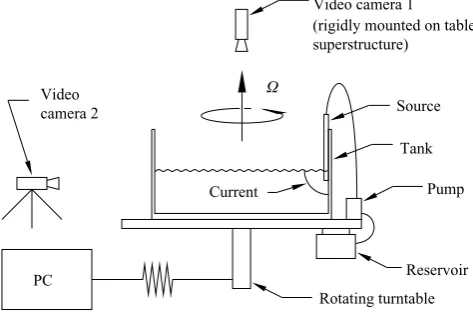
The goal of the experiments was to simulate estuarine discharges of buoyant fresh water into an environment of salty, denser, ocean water. The arrangement of the experimental small-scale facility is shown in figure 1.
Reservoir Pump Video camera 1 (rigidly mounted on table superstructure)
Video camera 2
PC
Source
Tank
Rotating turntable Current
[image:4.493.119.356.63.219.2]Ω
Figure 1.The small-scale experimental set-up.
Small-scale experiments Large-scale experiments
Radius RS= 0.4475 m RL= 6.5 m
Rotation rateΩ 0.5 rad s−16Ω62.5 rad s−1 0.0196 rad s−16Ω60.157 rad s−1
Flow rateq0 3.18 cm3s−16q0628.2 cm3s−1 200 cm3s−16q063972 cm3s−1
Reduced grav. accel.g 1.9 cm s−26g686 cm s−2 3.5 cm s−26g630.2 cm s−2 I, see (3.23) 0.07886I63.317 0.007326I60.388
Table 1. Summary of the ranges of the independent parameters in the small-scale and
large-scale experiments.
The tank was filled with salt water of density ρ2 representing the ocean water. Fresh water of densityρ1, withρ1< ρ2, was released from a small source mounted at the wall of the tank to simulate estuarine discharges. Fluid was released continuously and with a constant volumetric discharge rate,q0 (see table 1). The density difference between the fresh water and the salt water is characterized in terms of the reduced gravitational acceleration, g, defined by
g= ρ2−ρ1
ρ1 g, (2.1)
with g= 981 cm s−2.
visualization purposes the fresh water discharging at the source was dyed with food colouring while the ambient salt water was clear.
The experiments were filmed with two video cameras simultaneously. One camera was rigidly mounted on the superstructure of the rotating turntable and filmed the current from above the centre of the tank (figure 1). The second camera was positioned next to the turntable and filmed the flow through the transparent sidewall of the acrylic tank. This camera thus scanned the current height at the wall of the tank once per turntable revolution.
2.2. Large-scale experiments
The Coriolis Facility of the Laboratoire des Ecoulements G´eophysiques et Industriels (LEGI) at Grenoble, France, is the world’s largest rotating platform for the simulation of oceanographic flows in the laboratory. The total diameter of the platform is 14 m and the radius of the steel basin supported by the facility is RL= 6.5 m. The Coriolis Facility enables experiments which are to leading order non-viscous and dominated by background rotation, i.e. the Reynolds number is large while the Rossby number is small. Details of the technical specifications of the facility can be found at http://www.coriolis-legi.org.
We carried out 34 large-scale experiments. The ranges over which the experimental parameters were varied during these experiments are included in table 1. Each experiment on the large-scale facility was filmed with seven video cameras simultan-eously. These cameras were mounted at various appropriate locations on the rotating platform. Some cameras monitored sections of the tank from a few metres vertically above the fluid surface. Others were positioned at windows in the sidewall of the tank. Additionally several conductivity probes and ultrasonic profilers were mounted on the facility to measure the internal velocity and density structure of the currents.
The salt water in the tank was approximately 80 cm deep. Fresh fluid was supplied to the source mounted at the wall of the tank from storage reservoirs housed in the basement of the laboratory. The source and the supply system were made from commercially available drainage pipes of approximate diameter 15 cm.
3. Theoretical description of the problem
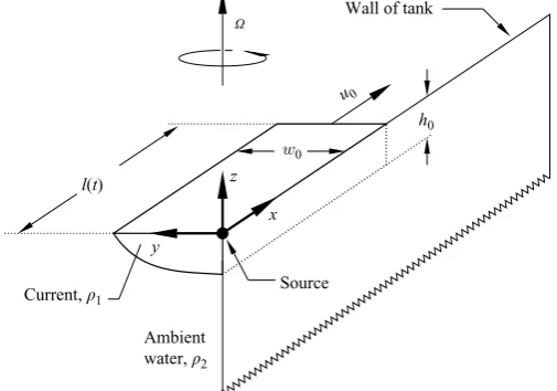
Figure 2 illustrates the geometry used to describe the motion of the current along the wall of the tank. The curvature of the circular wall is neglected, and a Cartesian coordinate system x, y, z is introduced as indicated in the figure. The origin of the coordinate system coincides with the outlet of the source from which the buoyant, fresh, fluid discharges. It is assumed that the velocity components in the y- and z-directions are negligible in comparison to the velocity component u in the x -direction. Further, we neglect all variations in the x-coordinate direction so that u= (u(y, z),0,0).
The pressure,p, is given by the hydrostatic relation
p=
gρ1(η−z), −h < z < η,
gρ1(h+η)−gρ2(z+h), z <−h, (3.1)
whereη =η(y) represents the free-surface elevation above z= 0 and the pressure at the free surfacez=η is taken asp= 0.
Current, ρ1
Ambient water, ρ2
x
y
z
u0
Wall of tank
Source
h0
w0
l(t)
[image:6.493.114.367.66.243.2]Ω
Figure 2.The nomenclature employed to develop the theoretical model for the current.
the current is in geostrophic balance,
2ρ1Ωu=−∂p
∂y, (3.2)
whereΩ is the rotation rate. From (3.1) one obtains
∂p ∂y =
⎧ ⎪ ⎨ ⎪ ⎩
gρ1∂η
∂y, −h < z < η, g(ρ1−ρ2)∂h
∂y +gρ1 ∂η
∂y, z <−h.
(3.3)
In the infinitely deep lower layer, i.e. for z <−h, there is no flow. Hence there the pressure gradient∂p/∂y= 0, and (3.3) for the lower layer yields
ρ1 ∂η
∂y = (ρ2−ρ1) ∂h
∂y. (3.4)
Comparison of (3.4) with the pressure gradient ∂p/∂y for −h < z < η in (3.3) then reveals that, in the current,
∂p
∂y = (ρ2−ρ1)g ∂h
∂y.. (3.5)
Substituting (3.5) into (3.2) gives
u=− g
2Ω ∂h
∂y, (3.6)
whereg is defined by (2.1). The potential vorticity,q, in the current is
q= 2Ω−∂u/∂y
h . (3.7)
potential vorticity does not have a major effect on the overall speed and shape of the current. Withq= 0 and (3.7), conservation of potential vorticity then implies that ∂u/∂y= 2Ω. Differentiating (3.6) with respect to y and then substituting for∂u/∂y in (3.7) gives
∂2h ∂y2 =−
4Ω2
g . (3.8)
Integration of (3.8) yields
h=−4Ω 2
2g y 2+
cy+d, (3.9)
wherec andd are constants. Conservation of angular momentum implies that u= 0 at the wally= 0. Hence, (3.6) implies ∂h/∂y= 0. Thusc= 0 and
h=h0− 2Ω2
g y
2, (3.10)
whereh0 is the (maximum) depth at the wall. Reference to (3.8) and (3.6) shows that this parabolic depth profile (3.10) implies that the current velocity
u= 2Ωy (3.11)
increases linearly with distance from the wall.
The current has maximum widthw0 where the interface (3.10) intersects the fluid surface, i.e whenh(y=w0) = 0. Thus (3.10) gives
w0 =
gh0 2Ω2
1/2
. (3.12)
Assuming that the width and depth of the current at any downstream location remain constant in time, continuity requires that the volumetric flow rate, q0, from the source must equal the volumetric flow rate across any cross-section of the current. Then
q0=
w0
0
h(y)u(y) dy, (3.13)
is independent of x. Substituting (3.10) and (3.11) into (3.13), one obtains after integration
q0 =
h0Ωw02− Ω3w4
0 g
. (3.14)
From (3.12) and (3.14) one finds
h0=
4Ωq0 g
1/2
, (3.15)
and then from (3.15) and (3.12)
w0=
gq0 Ω3
1/4
. (3.16)
The total current volumeV is given by
V =q0t =l
w0
0
wherel represents the length of the current. Carrying out the integration using (3.10) and then introducing (3.12) and (3.15) leads to
V =q0t =l
4q03/4
3g1/4Ω1/4. (3.18)
Equation (3.18) implies that the current travels at constant speed l/t=u0 and that the lengthl is given by
l= 3 4(q0g
Ω)1/4t. (3.19)
These scalings for the width, depth and velocity of the current are the same as those given in Davies et al. (1993) and, more recently, by Lentz & Helfrich (2002). However, since these authors used only scaling arguments they could not give explicit values for the constants in their expressions. The definition of Horner-Devine et al.
(2006) for the maximum depth in a geostrophic current is identical with the current depth obtained from our model in (3.15). The model of Avicola & Huq (2002), which is based on the assumption that the frontal dynamics are that of a Margules front, also yields the same current depth as that in (3.15). In terms of our nomenclature the current width derived by Avicola & Huq is w0= (1/√2)(gq0/Ω3)1/4 and this value is thus smaller by a factor 1/√2 = 0.707 than that found from (3.16). From (3.19) one sees that the constant propagation speed of the current head in our model is u0=l/t=3
4(q0gΩ)
1/4. In comparison, the speed of the current head found by Avicola & Huq isu0=
√
2(q0gΩ)1/4. Thus, their current speed is higher by a factor
√
2/(3/4) = 1.89 than that predicted by the present model.
The results above can be conveniently expressed in dimensionless form. We use the non-dimensional time T =Ωt and non-dimensionalize lengths by w0= (gq0/Ω3)1/4. The scale w0 is equivalent to the usual Rossby deformation scale, √gh0/Ω, for the flow based on the flow rate in the current. The deformation scale corresponds to the usual adjustment length based on potential-vorticity conservation. This can be seen as follows. Solving (3.15) for q0, substituting this expression into (3.19) and then solving for l/t=u0 shows thatu0 scales as √gh0. Equation (3.12) immediately reveals the usual adjustment scaling w0 ∝
√
gh0/Ω. Together with q0∝u0h0w0 the two scalings for u0 and w0 imply q0∝
√
gh0h0(
√
gh0/Ω). By substituting h0 in this expression by means of (3.15), rearranging and comparing with (3.16) one sees that√gh0/Ω∝(gq0/Ω3)1/4=w0. Hencew0is equivalent to the Rossby deformation radius based on the depth of the current.
Using capital letters to denote non-dimensional variables, (3.19) is written as
L= 3
4T . (3.20)
The dimensionless width is then given by
W = 1, (3.21)
and the dimensionless depth is
H = 2I5/4. (3.22)
Reference to (3.15) and (3.16), or to (3.22) with H=h0/w0, reveals that the quantity
I = Ωq 1/5 0
g3/5 , (3.23)
(3.15), (3.16) and (3.19) for the current depth, width and the length does not alter the form of the non-dimensional current width in (3.21). Neither does it affect the non-dimensional current depth given by (3.22) as long the definition of I in (3.23) remains unchanged. In (3.20), which gives the non-dimensional current length, the timeT =Ωt would be replaced by f t.
One can define a Rossby numberRo as
Ro= u0 Ωw0
, (3.24)
whereu0=l/t from (3.19), and a Froude numberFr as
Fr= √u0 gh0
. (3.25)
Using the expressions (3.15) forh0, (3.16) forw0 and (3.19) foru0 one finds
Ro= 3
4 = 0.75 (3.26)
and
Fr= 3
25/2 = 0.5303. (3.27)
The ratio of body forces and Coriolis forces is expressed by the ratio of the Rossby number and the Froude number and, with (3.26) and (3.27), one finds that
Ro
Fr =
25/2
4 =
√
2. (3.28)
If one uses the expressions of Avicola & Huq (2002) for the current width, depth and propagation velocity to calculate the Rossby number, the Froude number and the ratio of both, corresponding to the above expressions (3.26), (3.27) and (3.28), one findsRo= 2, Fr= 1 and, consequently,Ro/Fr= 2.
The current velocity u0=l/t from (3.19) together with (3.15) can also be used to define a Reynolds numberRe(w0, u0)
Re= w0u0
ν =
3q01/2g1
/2
4Ω1/2ν . (3.29)
Finally one can define an Ekman numberEk(h0) as
Ek(h0) = ν f h02
= νg
2f2q 0
= νg
8Ω2q 0
. (3.30)
Using the values given in table 1 together with ν= 0.01 cm2s−1 for the kinematic viscosity of water, the small-scale experiments turn out to have Reynolds numbers in the range 1006Re(w0, u0)65200 while the corresponding range for the large-scale experiments is 50006Re(w0, u0)6185 000. Similarly, the small-scale experiments have Ekman numbers in the range 1.34×10−56Ek(h
0)61.34×10⁻¹while the large-scale experiments have values in the range 4.47×10−56Ek(h
0)64.91×10⁻¹.
4. Experimental results
4.1. Introductory remarks
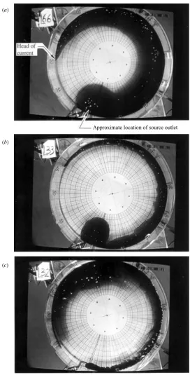
Figure 3(a–c) shows flow visualizations that are typical examples of currents observed in the small-scale facility for low, intermediate and high values of I. The pictures were obtained with the corotating camera 1 (figure 1) and show the currents viewed from above the circular tank, looking vertically downwards onto the fluid surface. The dyed current fluid appears dark in the pictures. The location of the source, where the buoyant current fluid is ejected, is indicated in figure 3(a) and it is the same in figures 3(b, c). The turntable rotates anticlockwise. The currents propagate cycloni-cally, i.e. also anticlockwise, around the circumference of the tank. The calibration grid visible in each picture was attached to the table top underneath the transparent bottom of the tank. The angle of each grid sector is 0.1 radians and the separation between two successive calibration circles is 5 cm.
4.1.1. Qualitative aspects of the current shape: small-scale currents
A comparison of figures 3(a–c) reveals that the currents look qualitatively different for different values ofI. The current shapes shown are characteristic for the different values of I. After some experience, it is possible to estimate the value of I for any particular current by simple inspection of a flow visualization. Recall that, because of (3.23) and (3.30), the lowest values of I correspond to the highest values of Ek and vice versa. However, it is the currents, such as the one shown in figure 3(c), having a low Ek (largeI) value which are most closely governed by geostrophy. For such currents, the flow in the initial stage looks similar to the currents in figures 3(a) and 3(b). However, at some point the frontal portion of the currents separates from the source and is advected downstream with the flow. As a result a current with a constant width, as predicted by our model, is left behind. We believe that it is the type of current after the frontal portion has separated that represents a current closely governed by a geostrophic balance and which is not significantly affected by viscous effects. The currents in figures 3(a) and 3(b) do not have a constant width. The reason for this is probably that the associated values of the Ekman number are too large (low I) and the currents are not sufficiently well governed by geostrophy. This will be discussed in depth in§4.5, where the data for the current width are analysed.
The observations have shown that anticyclonically (i.e. clockwise) spinning gyre is formed at the upstream end of the current in the immediate vicinity of the source. For the currents in figures 3(a) and 3(b) it was observed that the diameter of this bulge region grows continuously with time; in these figures the diameter of the bulge is about 25 cm. Similar gyres were observed and studied experimentally by Avicola & Huq (2003b) and Horner-Devineet al. (2006). Nof & Pichevin (2001) investigated the issue theoretically and predicted the existence of the growing, recirculating, bulge region. As a consequence of the gyre formation some fluid is lost from the main body of the current and this must result in discrepancies with the predictions of our model. For instance, it is expected that drainage of fluid out of the main current will tend to decrease the propagation speed of the current. Hence, the current will no longer have the constant speed predicted by our model.
(a)
(b)
(c)
[image:11.493.116.389.56.592.2]Approximate location of source outlet
Figure 3.Flow visualizations showing currents (dark fluid) flowing around the wall of the
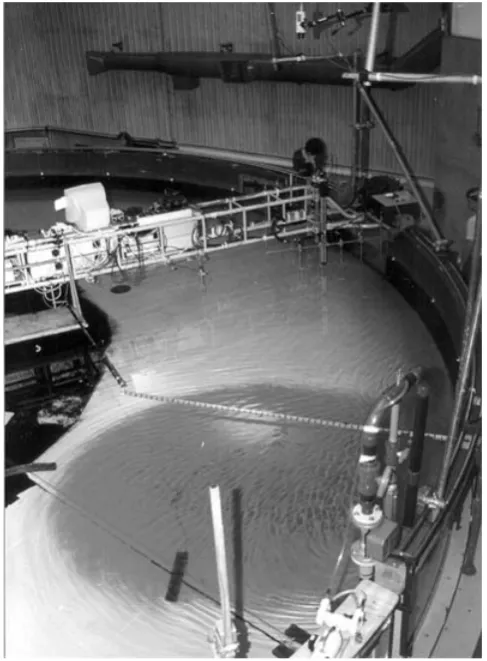
Figure 4. Part of a large-scale current in the Coriolis Facility.
table 1 in Avicola & Huq (2003b) that their experiments were in the parameter regime 0.1376I60.397. Similarly, one determines 0.0776I60.331 for the experiments of Horner-Devine et al. (2006) from tables 1–3 in the appendix of their paper. Hence, all the experiments of Avicola & Huq (2003b) and Horner-Devineet al. (2006) were within the same parameter region as our currents shown here in figures 3(a) and 3(b). None of their experiments had values as high as I= 2.776, the parameter regime of the current in figure 3(c) where we observed a bulge with a constant diameter and currents of constant width. It was noted that the separation of the frontal portion of a current at high I, as in figure 3(c), often happens relatively late during the experiment. Hence, in order to carry out further experiments in the parameter regime of g, q0 and Ω resulting in largeI,i.e.∼2–3, it would be desirable to have a larger tank available than the 1 m diameter tank used in the present small-scale experiments.
4.1.2. Qualitative aspects of the current shape: large-scale currents
0 500 1000 1500 2000
t (s)
500 1000 1500 2000 2500 3000 3500 4000
l
(cm)
[image:13.493.137.376.56.223.2]3972 3000 1500900 600 400 300 200
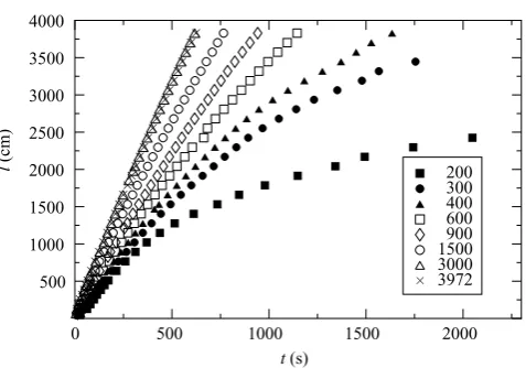
Figure 5.Typical raw data sets displaying the current length, l, as a function of time, t,
for eight large-scale experiments with different flow rates, q0, but the same rotation rate, Ω= 0.1571 rad s−1, and equal reduced gravity, g= (3.57±0.15) cm s−2. The numbers in the key are the values ofq0 in cm3s−1.
is flowing away from the viewer. The exact experimental conditions relating to the current shown are not available since they were not recorded when the picture was taken. However, figure 4 reveals that the current is relatively narrow in comparison to the gyre diameter near the source. Reference to the picture sequence for small-scale currents in figure 3(a–c) suggests that I was of intermediate value because a comparison of the large-scale current of figure 4 shows that it looks very similar to the small-scale current with the intermediate value,I= 0.3264, in figure 3(b).
4.2. Current length
Figure 5 shows eight typical raw-data sets for the current length l as a function of timet. The data are from large-scale experiments with different volumetric discharge rates q0 but equal rotation rate Ω= 0.1571 rad s−1 and equal reduced gravity g= (3.57±0.15) cm s−2. It can be seen that the currents with higher discharge rates q0 propagate faster. Their velocity is almost constant during propagation along the entire 40 m circumference of the tank. Currents with lower values ofq0 initially have an approximately constant propagation velocity but gradually begin to slow down during the experiment.
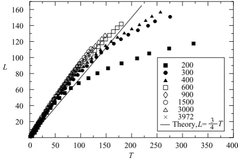
Figure 6 redisplays the data of figure 5 in non-dimensional form. The solid line superposed on the figure is the theoretical prediction L=3
4T from (3.20). The figure reveals that experiment and theory are in quite good agreement. The experimentally measured current length at early times T grows faster than predicted but begins to slow down at later times. The reason for this initial velocity excess and subsequent gradual deceleration will be discussed in§ §4.4.2 and 4.5.6.
50 100 150 200 250 300 350 400 T
0 20 40 60 80 100 120 140 160
L
Theory,3972 L= 3000 1500900 600 400 300 200
[image:14.493.118.358.60.222.2]3 4 T
Figure 6. The data for the current length, l, of figure 5 in non-dimensional form: the
non-dimensional current length,L, is shown as a function of the non-dimensional time,T, for eight experiments with different flow rates q0 but equal rotation rate,Ω= 0.1571 rad s−1, and
equal reduced gravity,g= (3.57±0.15) cm s−2. The numbers in the key are the values ofq0in
cm3s−1.
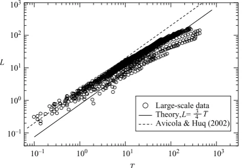
each other. Hence the small-scale and large-scale experiments display corresponding behaviour, suggesting that the dynamics of the experiments are the same at both scales. The dashed line superposed onto figures 7 and 8 represents the theoretical result for the current speed of Avicola & Huq (2002). Their results have been re-expressed in our nomenclature, where the dashed line is given byL= 2T. This line was obtained by interpreting the current speedc in expression (5) of Avicola & Huq (2002) asc=l/t, so thatl=ctcorresponds to expression (3.19) in the present paper. The current length l was then non-dimensionalized using the Rossby deformation scale given in equation (4) of Avicola & Huq (2002). Figure 7 shows that, for the small-scale experiments, our model predicts the propagation of the current head slightly better overall than the model of Avicola and Huq. For the large-scale data shown in figure 8 the prediction of Avicola and Huq seems to give slightly better agreement. However, this apparent better agreement is slightly misleading. As will be discussed in §4.4.2, the currents have, initially, a velocity excess due to the measured along-wall depth profile. If this is taken into account then it appears justifiable to conclude that overall the experimental data for the current speed, in both the small-scale and the large-scale experiments, is in better agreement with our present model than with the model of Avicola & Huq (2002).
4.3. Current velocity
Figure 9 shows examples of the ratio of the experimentally measured non-dimensional mean velocityUe
0 of the current head and the theoretically predicted current velocity Ut
0=L/T = 3
4 from (3.20). The velocity data shown were obtained from the analysis of the eight experiments whose results were displayed in figures 5 and 6 (Ω= 0.1571 rad s−1,g= (3.57±0.15) cm s−2).
It should be emphasized that Ue
T 103
102
101
100
10–1
10–1 100 101 102 103
L
Avicola & Huq (2002) Theory,L=
[image:15.493.142.374.57.228.2]Small-scale data 3 4 T
Figure 7.Summary of the data for the non-dimensionalized current length Las a function
of the non-dimensional timeT, for the small-scale experiments. The solid line represents the theoretical prediction of (3.20).
T 103
102
101
100
10–1
10–1 100 101 102 103
L
Avicola & Huq (2002) Theory,L=
Large-scale data 3 4 T
Figure 8.Summary of the data for the non-dimensionalized current length,L, as a function
of the non-dimensional time,T, for the large-scale experiments. The solid line represents the theoretical prediction of (3.20).
To see typical maximum magnitudes of these fluctuations refer to similar curves shown in Davieset al.(1993), which were obtained in this way.
Figure 9 reveals that the data for all eight experiments collapse reasonably well for timesT >25. It can be seen how the current velocity decreases with timeT; it is not constant as predicted by our simple geostrophic model. For times 25< T <175 the current is faster than predicted by a factor between about 1 and 1.5. In§3 it was noted that the current speedUt
0 predicted by the model of Avicola & Huq (2002) is higher by a factor 1.89 than the speed predicted by the present model. If the data in figure 9 were rescaled to account for this then the position of the dotted line, which indicates exact agreement between experiment and theory, would shift to Ue
[image:15.493.137.374.284.448.2]50
0 100 150 200 250 300 350
T 0.5
1.0 1.5 2.0 2.5 3.0
U0
e/U
0
t 39723000
[image:16.493.121.358.63.220.2]1500900 600 400 300 200
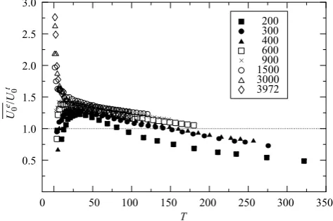
Figure 9. The ratio of the measured non-dimensional current mean velocity U0e and the
predicted velocityUt
0= 0.75, as a function of T. The numbers in the key are the values ofq0
in cm3s−1.
Note the behaviour displayed by the data in figure 9 during the initial phase of the experiments, for timesT <25. Here the data points do not collapse: it can be seen that the data points for experiments with different discharge rates q0 display qualitatively different behaviour. Forq0 6900 cm3s−1the data points approach the common curve for T > 25 from below, while they approach it from above for q0 > 1500 cm3s−1. The displayed data represent experiments with flow rates 200, 300, 400, 600, 900, 1500, 3000 and 3972 cm3s−1 and the associated values of I are, respectively, 0.213, 0.231, 0.249, 0.270, 0.288, 0.313, 0.354 and 0.387. The change in behaviour occurs between 900 and 1500 cm3s−1 and, thus, in the interval 0.288< I <0.313. The associated ranges of the Reynolds numberRe(w0, u0) and the Ekman numberEk(h0) are 10 650<Re(w0, u0)<13 943 and 1.22×10⁻⁴< Ek(h0)<1.98×10⁻⁴. However, the rotation rate (Ω= 0.1571 rad s−1) and the reduced gravity (g≈3.57 cm s−2) have the same values for all the experiments in figure 9. Consequently, the interval where the transition in the behaviour is observed may be different for a series of experiments having different combinations of values of Ω and g. We do not at present have data from other appropriate series of experiments available to address this issue in more detail.
4.4. Current height
4.4.1. Introductory remarks
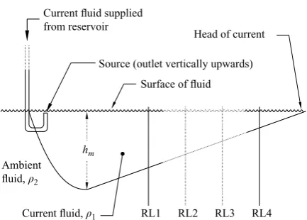
Our model predicts that the current heighth0 at the wall of the tank (see figure 2 and (3.15)) is independent of the x-coordinate. Its value is equal to the current depth predicted by Avicola & Huq (2002) and the maximum depth in a geostrophic current given in Horner-Devine et al. (2006). However, the videos recorded with camera 2 of figure 1, through the sidewall of the tank, reveal that the current height decreases between the source region and the current head. A schematic illustration of the observed height profile at the wall (y= 0), in the (x, z)-plane of figure 2, is shown in figure 10.
Current fluid supplied from reservoir
Surface of fluid Source (outlet vertically upwards)
Current fluid, ρ1 Ambient
fluid, ρ2
RL1 RL2 RL3 RL4
hm
[image:17.493.145.362.56.211.2]Head of current
Figure 10.A side-view of the current as recorded by video camera 2, shown in figure 1. The
diagram shows how the current height changes with the along-wall distancex from the source to the current head, i.e. it gives the height profile at the wall (y= 0) in the (x, z)-plane of figure 2.
and the head of the current corresponds to the circumference of the tank. It was observed that the current height has a maximum,hm, just downstream of the source. The distance x between the source and the position where the maximum height is observed is around 1–5 cm in the small-scale facility and around 10–50 cm in the large-scale facility. The maximum heighthmis, typically, in the range 0.5 cm < hm<9 cm for the small-scale experiments and in the range 1.5 cm < hm<50 cm for the large-scale experiments. This heighthm was observed to be constant throughout each experiment and was used for comparison with the theoretical prediction ofh0 given by (3.15) and in non-dimensional form by (3.22).
4.4.2. Height profile of the currents along the wall of the tank
For the small-scale experiments we measured the maximum current height and the current height at four further reference locations along the circumference of the tank. The reference locations, identified as RL1–RL4 in figure 10, were positioned at 1.5, 2.5, 3.5 and 4.5 radians downstream of the source. It was not possible to obtain corresponding data for the large-scale experiments by viewing through the sidewall windows of the Coriolis Facility, as the dye in the current became too diluted at the interface between the current and the ambient fluid, making it impossible to define the current boundary reliably by visual inspection.
0 0.1 0.2 0.3 0.4 0.5 0.6 0.7 0.8 0.9 1.0
x/(2πRS)
0.4 0.5 0.6 0.7 0.8 0.9 1.0 1.1
h
(
x
)/
hm
[image:18.493.120.359.62.228.2]h(x)/hm = –0.65x/(2πRS)+1.09
Figure 11. The relative current height,h(x)/ hm, for the small-scale experiments as a
function of the non-dimensional distancex/(2πRS) from the source.
0 0.5 1.0 1.5 2.0 2.5 3.0
I 0
1 2 3 4 5 6 7
H0 28.1220.0 10.0 3.18 Small-scale exps.
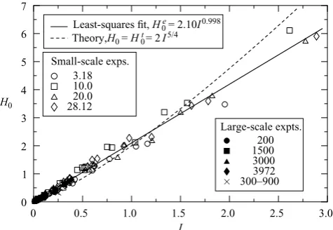
300–9003972 3000 1500200 Large-scale expts. Theory,H0 = H0t= 2I5/4
Least-squares fit, H0e= 2.10I0.998
Figure 12.Non-dimensional maximum current height near the source,H0=hm/RD, as a
function ofI. The numbers in the key are the values ofq0 in cm3s−1.
4.4.3. Scaling of the current height with the parameter I
In order to facilitate a comparison between the experiments and the theoretical model of §3, the measured maximum current heighthm is identified with the current heighth0 predicted by (3.15). Figure 12 gives a summary of the measured values for hm in non-dimensional form, in terms ofH0=hm/RD as a function of I. (Recall that the current depths predicted by our present model, that predicted by the model of Avicola & Huq (2002) and that defined by Horner-Devineet al.(2006) are the same.) A least-squares fit to the data points for the small-scale and large-scale experiments gives
He
0 = 2.10I
0.998, (4.1)
[image:18.493.121.359.273.437.2]0 0.05 0.1 0.15 0.2 0.25 0.3 0.35 0.4 0.45 I
0 0.5 1.0 1.5 2.0 2.5 3.0 3.5 4.0
H0
e/H
0
t
Ω= 0.0196 rad s–1 Ω= 0.0523 rad s–1 Ω= 0.1571 rad s–1
[image:19.493.139.371.42.217.2]Envelope of large-scale data
Figure 13. The ratio of measured current height,H0e, and theoretical height,H0t, given by
(3.22) for the large-scale experiments as a function ofI.
Envelope of large-scale data
0 0.5 1.0 1.5 2.0 2.5 3.0
I 0
0.5 1.0 1.5 2.0 2.5 3.0 3.5 4.0
H0
e/H
0
t
[image:19.493.139.373.260.417.2]Ω= 0.5 rad s–1 Ω= 1.0 rad s–1 Ω= 1.5 rad s–1 Ω= 2.5 rad s–1
Figure 14.The ratio of measured current height,H0e, and theoretical height,H0t, as given by
(3.22) for the small-scale experiments as a function ofI.
Figures 13 and 14 identify the particular experiments responsible for this discre-pancy between experiment and theory. The two figures display the ratio of the measured non-dimensional height He
0 and the non-dimensional predicted height H0t as a function of the non-dimensional parameterI. The data for the large-scale experi-ments are shown in figure 13 while those for the small-scale experiexperi-ments are shown in figure 14. For good agreement between experiment and theory, H0e/H0t= 1. In both figures the data for different values of the rotation rate Ω are identified by different types of marker. In order to facilitate an easy comparison between the data for the large-scale and the small-scale experiments in these figures an envelope has been drawn around the large-scale data of figure 13 and this envelope has been superimposed onto figure 14.
Figures 13 and 14 reveal that for both large-scale and small-scale experiments the agreement between experiment and theory improves substantially with increasing values of the parameterI. For very low values,I <0.05, the experimentally measured value He
Ek(h0) 101
100
10–1
10–5 10–4 10–3 10–2 10–1 100
H0
e/H
0
t
Small-scale expts.
Ω= 0.0196 rad s–1 Ω= 0.5 rad s –1 Ω= 1.0 rad s–1 Ω= 1.5 rad s–1 Ω= 2.5 rad s–1 Ω= 0.0523 rad s–1
Ω= 0.1571 rad s–1
Large-scale expts.
Least-squares fit, H0
e
/H0
t
[image:20.493.125.361.64.228.2]= 3.45Ek(h0) 0.124
Figure 15. The ratio of the measured current height,H0e, and the theoretical height,H0t, given
by (3.22) as a function of the Ekman number,Ek(h0), defined by (3.30). A summary of all the
data for the large-scale and small-scale experiments is shown.
also show, in particular, that in both sets of experiments agreement with theory is very good for runs with higher rotation rates while it is less favourable for the lower rotation rates. This suggests that currents with low values of I are not governed by geostrophic balance and, consequently, cannot be described accurately by our model. It is these data points for low values of I coupled with low rotation rates which are responsible for the deviation of the least-squares fit (4.1) from the predictions of our model in (3.15) and (3.22).
Inspection of (3.23) reveals that experiments with low values of I are those for which the discharge rate q0 is small and for which the reduced gravity g is large. Reference to (3.15) shows that these currents are expected to be shallow. Hence, it is to be expected that the motion of currents with decreasing values ofI will be subject to increasing viscous effects; this is verified in the following section.
4.4.4. Scaling of the current height with the Ekman number
The Ekman number Ek(h0) based on the current height h0 of (3.15) is defined by (3.30). Figure 15 displays the ratio of the measured current height He
0 and the theoretical height Ht
0 as a function of Ek(h0). The summary of all the data for the large-scale and small-scale experiments is shown. The figure reveals that agreement between experiment and theory is best for the smallest Ekman numbers, i.e when viscous effects are negligible. Agreement deteriorates with increasing Ekman number, i.e. when viscous effects become important. A comparison of the scalings for Ω, q0 and g in (3.23) and (3.30) reveals that the smallest values of I correspond to the largest values ofEk(h0). Hence, the data points at higher values ofEk(h0) in figure 15 correspond to data points with lower values ofI in figures 13 and 14.
The data in figure 15 collapse onto a single straight line. Hence, the ratio He
0/H0t scales with the Ekman numberEk(h0). The solid line is a power-law least-squares fit given by
He
0 Ht
0
15
10
5
0
Radial distance from w
all (cm)
Wall of tank
Boundary of current at t0 and also
[image:21.493.113.396.50.291.2]appox. boundary at t0 + 10∆t
Figure 16.Typical surface-velocity profiles obtained from the observation of small tracer
particles advected downstream with a current in the small-scale facility. The profiles were collected at 1.5 radians, corresponding to 67 cm downstream of the source. The experimental conditions are Ω= 1.0 rad s−1, g= 16 cm s−2, q0= 20 cm3s−1 yielding, I= 0.34. The time
intervalt between two successive profiles is 0.5 s.
4.5. Current width
4.5.1. Introductory remarks
Measuring the position of the current head and the current height is straightforward, as seen in § §4.2 and 4.4. However, measurement of the current width is more involved since the edge of the current seen on the fluid surface is qualitatively different depending the value ofI; this dependence was discussed in§4.1.1.
In particular, for currents with low values of I the width identified and seen on the fluid surface by the outline of the dyed fluid does not represent the current width relevant to the dynamics of the geostrophic problem. This question is addressed by considering the region where the bulk of the fluid motion in the current takes place. To identify this region surface-velocity profiles for the currents were obtained.
4.5.2. Surface-velocity profiles
The surface velocity of the currents was determined by measuring the motion of small tracer particles floating on the surface of the current. The tracer particles were dropped onto the fluid surface in a straight line radially across the current. The particles were then advected downstream with the local surface-flow velocity.
Width of main body of
current
Apparent current width as seen when viewing
from above
Reflection from wall of tank
Reflection from bottom of tank
Boundary between main body of current and ambient fluid
Vertical light sheet
Direction of propagation Current
[image:22.493.80.400.57.414.2]Illuminated cross-section of current
Figure 17. Photograph of the cross-section (in a (y, z)-plane; see figure 2) of a large-scale
current illuminated by a vertical light sheet, as illustrated in the diagram below the photograph. The photograph was taken at approximately 0.844 radians, corresponding to 5.488 m, downstream of the source during an experiment with Ω= 0.1571 rad s−1, g= 8.5 cm s−2,
q0= 3000 cm3s−1andI= 0.216.
velocity profiles illustrate that the flow velocity is largest in a substantially narrower near-wall zone which is only about 8–10 cm across. In this near-wall zone the current is also deepest and, hence, this is the region where the bulk of the fluid motion takes place. Consequently, the width of the near-wall zone is the appropriate measure of the current width for the flow dynamics.
4.5.3. Cross-sectional illumination of currents
of the photograph is due to light reflected from the wall of the tank; the very bright horizontal and slightly curved line in the lower half of the photograph represents light reflected from the bottom of the tank. They-coordinate of figure 2 corresponds approximately to the direction horizontally across the page.
Figure 17 shows that the current is deepest at the wall of the tank, as expected from (3.10). We have not attempted quantitative comparisons between the parabolic profile given by (3.10) and visualizations such as that in figure 17. The photograph was taken by a camera positioned a few centimetres above the fluid surface and angled slightly downwards. Consequently, the cross-section as it appears in figure 17 is slightly distorted.
Again, figure 17 suggests that the width of the main current is substantially smaller than the apparent total width identified by the fluorescein illumination. There is a clear boundary between the fluid which constitutes the main body of the current and the adjacent fluid contaminated by fluorescein. This boundary is only seen on visualizations of the cross-sections and is not visible when viewing the current from above, as in figures 3(a–c) or figure 4. This corroborates the conclusion of§4.5.2 that data for the current width based on measuring the width seen on the liquid surface in dye-visualization experiments give substantial overestimates. For example, the main current shown in figure 17 is only about half as wide as the total apparent width suggested by the fluorescein illumination. This is consistent with the discussion of figure 16 in §4.5.2 concerning how the surface-velocity profiles for a current with a similarly low value of I suggest that the main current is only about half as wide as the width indicated by the outline of the food colouring. The shallow surface layer outside the main body of the current is fluid in the surface Ekman layer produced by the (small) stress at the surface.
4.5.4. Error estimates for the measurement of the current width
For currents with low to intermediate values ofI (figures 3aand 3b), measurements of the width of the near-wall zone discussed in§4.5.2 were used for comparison with our model. Figure 16 shows that the transition between the near-wall zone and the outer current zone is gradual. Hence, the definition of the width of the near-wall zone involves a degree of ambiguity. Typical maximum errors resulting from this uncertainty for the measurement of the current width from surface-velocity profiles are estimated to be no larger than 10 %–15 %.
For low values of I (figure 3a) the current width was always measured by con-sidering surface-velocity profiles only. However, for intermediate values ofI(figure 3b) an additional second measurement was taken. For these currents the experiments revealed that the narrowest width, at the contraction where the water from the gyre begins its motion along the wall, agrees well with the width obtained from surface-velocity profiles. Because of this we measured both quantities for currents with intermediate values ofI and we then used their average as the current width for comparison with the theory.
2 10 12
RD(cm)
0 2 4 6 8 10 12
w0 e (cm)
28 20 10
3.18 Avicola & Huq (2002)
w0e = RD
[image:24.493.116.366.63.236.2]4 6 8
Figure 18. The measured current width,we0, as a function of the Rossby deformation scale RD, for the small-scale experiments. The numbers in the key are the values ofq0 in cm3s−1.
At high values ofI there is another mechanism which can result in the data being biased towards an overestimation the current width. At high values of I, i.e. when g is small while q0 and Ω are large, the currents are deep and fast moving. For such currents, shear instabilities appear on the boundary between current fluid and ambient fluid. These instabilities can be seen in figure 3(c) in the region 0.2–1.0 radians downstream (two to ten sectors of the reference grid) of the source. The figure reveals that the amplitudes of these instabilities are of the order of up to 10– 20 mm. This translates into 100 %–200 % of the total width of these narrow currents in the small-scale facility. Together with the absolute measurement error, the total relative measurement error can lie within roughly 100 %–300 % for the currents with the highest values of I. The corresponding relative error for large-scale currents is substantially smaller. The magnitude of the amplitudes of the shear instabilities for currents with highest values ofI in the large-scale facility is of the same magnitude as in the small-scale facility. However, the currents in the large-scale facility are typically at least about 200 mm across. Hence, the relative error associated with with the shear instabilities is at least one order of magnitude smaller for the large-scale currents than for the small-scale currents.
4.5.5. Scaling of the current width with the parameterI
Figure 18 displays the experimental data for the current width measured in the small-scale experiments. The theoretical model in §4 yields W=w0e/RD= 1. Hence, good agreement between experiments and theory requires we
0=RD, identified by the solid line in figure 18. The figure reveals satisfactory agreement between experiment and theory. The dotted line in figure 18 represents the theoretical prediction for the current width from the model of Avicola & Huq (2002), which is given by w0= (1/
√
2)(gq0/Ω3)1/4in our nomenclature. Figure 18 shows that the present model describes the experimental data slightly better than that of Avicola & Huq (2002).
Figure 19 shows the ratio we
0/RD as a function of the non-dimensional parameter
0 0.5 1.0 1.5 2.0 2.5 3.0 I
0.5 1.0 1.5 2.0 2.5 3.0 3.5 4.0
w0 e/R
D
28 20 10
[image:25.493.131.384.57.233.2]3.18
Figure 19. The ratio of the measured and predicted current widths,we0/RD, as a function of I for the small-scale experiments. The numbers in the key are the values ofq0 in cm3s−1.
50 100 150 200 250 300 350
RD(cm)
0 50 100 150 200
w0 e (cm)
3972 3000 1500 300–900 200 Avicola & Huq (2002)
[image:25.493.130.383.279.450.2]w0e = RD
Figure 20.The measured non-dimensional current width, we0, as a function of the Rossby
deformation scale,RD, for the large-scale experiments. The numbers in the key are the values
ofq0 in cm3s−1.
the interface between current fluid and ambient fluid and it was seen that these can introduce relative errors of order 100 %–300 % for the narrowest currents at highest values ofI in the small-scale facility. These large relative errors probably explain why agreement between experiment and theory in figure 19 is generally better at lower values ofI rather than at higher ones.
0 0.05 0.10 0.15 0.20 0.25 0.30 0.35 0.40 0.45 0
0.2 0.4 0.6 0.8 1.0 1.2 1.4 1.6 1.8 2.0
3972 3000 1500 300–900 200
I w0
e/R
[image:26.493.113.370.63.231.2]D
Figure 21. The ratio of the measured and predicted current widths,we0/RD, as a function of I for the large-scale experiments. The numbers in the key are the values ofq0in cm3s−1.
narrower currents, figure 20 shows that the present model describes the experimental data slightly better than the model of Avicola & Huq (2002). For very wide currents, with w0e>150 cm, our model overpredicts the experimental data and the prediction of Avicola & Huq (2002) appears to describe the experiments somewhat better.
Figure 21 shows the ratio we
0/RD as a function of the non-dimensional parameter
I for the large-scale experiments. The data show that the quality of the agreement between experiment and theory is, essentially, the same over the entire interval 0 6 I 6 0.4 for which large-scale experiments were carried out. However, the data scatter is somewhat higher for smaller than for higher values ofI.
Figure 22 shows a summary of all data points for we
0/RD for the small-scale and the large-scale experiments. The figure reveals that agreement is overall most favourable for the large-scale experiments with low values ofI. This observation can be understood in terms of the measurement errors discussed in§4.5.2. For small-scale experiments at high values of I the shear instabilities at the current boundary lead to very large relative errors. This is reflected by the data in figure 22 and this source of error cannot be eliminated from the measurements. At lower values of I, when currents are generally slow, errors from the shear instabilities are no longer significant. The main source of error is now that associated with current fluid spilling out of the main current and contaminating the ambient fluid, as discussed in connection with figures 16 and 17. However, this source of error can be largely suppressed for currents with low to intermediate values of I if one measures the current width, as discussed in§4.5.2. This leads to smaller errors and, hence, better agreement between experiment and theory for low values of I.
4.5.6. Scaling of the current width with the Reynolds number
Figure 23 displays the summary of all data forwe
0/RD from the large-scale and the small-scale experiments as a function ofRe(w0, u0), defined in (3.29). The data points below aboutRe(w0, u0) = 5×10³are those for the small-scale experiments while those above this value are from the large-scale experiments.
3972 3000 1500 300–900 200 Large-scale data
28 20 10
3.18 Small-scale data
0 0.5 1.0 1.5 2.0 2.5 3.0
I 0
0.5 1.0 1.5 2.0 2.5 3.0 3.5 4.0
w0 e/R
[image:27.493.93.423.61.234.2]D
Figure 22.Summary of all small-scale and large-scale data for the ratio of the measured and
predicted current widths,we0/RD, as a function ofI. The numbers in the key are the values of
q0in cm3s−1.
102 103 104 105
Re (w0, u0)
10–1 100 101
3972 3000 1500 300–900 200 Large-scale data
28 20 10
3.18 Small-scale data w0
e/R
D
Figure 23.Summary of all small-scale and large-scale data for the ratio of the measured
and predicted current widths,we0/RD, as a function of the Reynolds numberRe(w0, u0). The
numbers in the key are the values ofq0 in cm3s−1.
Re(w0, u0)6103 again reflects measurement errors. It does not reflect an increased importance of viscous effects in comparison with the predictions of our inviscid model. Comparison of figures 23 and 22 shows that the data points for Re(w0, u0)6103 correspond to those with large values ofI. These points are subject to large relative measurement errors arising in association with the shear instabilities at the boundary of the currents.
[image:27.493.133.384.297.473.2]cannot be reflecting increased turbulent mixing of current fluid and ambient fluid at their interface for high Reynolds numbers; turbulent mixing would tend to result in overestimates for the experimentally measured current width we0. Consequently one would expectwe
0/RD>1, rather thanw0e/RD<1 as displayed by the data in the figure. When viscous effects are important, the fluid on the current surface is no longer governed by geostrophy. As a consequence this fluid can leak out of the main current. This results in the current width seen on the fluid surface being greater than the width relevant to the current dynamics. The current width is then no longer constant because fluid draining out of the current spreads across the surface. The current width as seen on the fluid surface thus becomes a function of time. Our observations have shown that this is the case for low to intermediate values ofI, i.e. for the two current types shown in figures 3(a) and 3(b). As discussed earlier, we measured the growth of the current width identified by the dye visualization experiments on the fluid surface, as a function of time at various reference locations RLi (figure 10) distributed along the wall of the tanks of the small-scale and the large-scale facilities. The data analysis showed that the surface width at each reference location RLi grows roughly as, (t∗)0.5 wheret∗=t−tRLandtRLis the time of arrival of the current head at reference location RLi. The result (t∗)0.5 confirms the corresponding measurements of Lentz & Helfrich (2002, p. 264). In § §4.2 and 4.3 it was observed that the currents slow down during the later stages of each experiment. This deceleration is a consequence of the leakage of fluid out of the main current. When fluid leaks out of the current the assumption of mass conservation for the main current in (3.13) and (3.17) is no longer valid.
5. Froude number
In§4.3 it was observed that the velocity of the current head decreases with timeT. We have calculated experimental values for the Froude number, Fr(Ti) =ue0/
√
ghm, based on the measured current mean velocity ue
0=li/ti and the measured maximum depthhmnear the source. The results obtained in this way are displayed in figures 24(a) and 24(b) for the small-scale and the large-scale experiments, respectively. The figures reveal that, for both sets of experiments, the Froude number is in the approximate range 0.16Fr61.51, and they illustrate how Fr decreases with time T. For the majority of runs the Froude number had value just below a 0.8 at the beginning of the experiment. This is reflected in the two figures through the very high concentrations of data points around T = 0,Fr= 0.8.
In these figures the data points for the different runs have been grouped into three different sets according to their values of the parameter I. Both figures reveal that there is a general trend for the Froude number to adopt lower values for smaller values of I. Low values of I correspond to high values of the Ekman number and, hence, to the parameter regime where viscous effects become increasingly important and where our inviscid model is no longer valid.
For the vast majority of all data points for the highest values of I (lowest Ek) the Froude number lies within the interval 0.356Fr60.78. The solid lines, given by
100 200 300 I > 0.2 0.05 < I≤ 0.2 0 ≤I≤ 0.05 Large-scale data
Fr = 0.85T–0.09
Small-scale data Fr = 1.2T–0.22
0 200 400 600
T T
0
(a) (b)
0.2 0.4 0.6 0.8 1.0 1.2 1.4 1.6
Fr
I > 1.0 0.5 < I≤ 1.0 0 ≤ I≤ 0.5 Small-scale data
Fr = 1.2T–0.22
Large-scale data Fr = 0.85T–0.09
[image:29.493.95.419.58.392.2]0 0 0.2 0.4 0.6 0.8 1.0 1.2 1.4 1.6
Figure 24. Froude numberF as a function of the non-dimensional time,T, for (a) the
small-scale experiments and (b) the large-scale experiments.
and large-scale experiments. The dotted line in figure 24(a) corresponds to the solid line in figure 24(b) andvice versa.
Our experimental result, that the majority of data for the Froude number lie within 0.356Fr60.78, is overall in good agreement with the predicted value ofFr= 0.5303 (3.27). Our values for the Froude number are lower than the value Fr≈√2 = 1.41 obtained by Martin & Lane-Serff (2005), who extended the theory of Benjamin (1968) to rotating currents, and they are also lower than the valueFr= 1 predicted by Shin
et al. (2004). In comparison, the dam-break experiments of Griffiths & Hopfinger
the value predicted by our model. However, it should be emphasized that this does not imply that our model necessarily describes the experiments better at larger T than that of Avicola & Huq (2002). The reason for this is that the current slows down because of the drainage of fluid from the main current due to the growing bulge region near the source together with the additional drainage near the current surface identified in§4.5.6. Because of this drainage the assumption of volume conservation underlying our model, and also the model of Avicola & Huq (2002), is no longer valid.
6. Summary and conclusions
Laboratory simulations investigating the influence of the rotation of the earth on the dynamics of gravity-driven surface currents developing from fresh-water river discharges into the ocean have been described. Two complementary studies with experiments on substantially different spatial scales have been performed and the data collected in both studies have been compared with each other.
A simple geostrophic model for the flow was developed to predict the current height, width and velocity as a function of the relevant independent parameters governing the flow. The scalings obtained are the same as those previously deduced by Davies
et al. (1993) and, more recently, by Lentz & Helfrich (2002) on the basis of scaling
arguments. However, since these authors used scaling arguments only, they were unable to give values for the constants missing from their proportionality relations. Our new model yields values for these constants and they have been compared with corresponding values obtained by Avicola & Huq (2002) and Horner-Devine et al.
(2006) wherever possible. Our theoretical analysis yielded a set of non-dimensional parameters suitable to summarize the measured data and to collapse the corresponding results from large-scale and small-scale experiments onto single lines. Our predictions are, generally, in good agreement with our experimental data. It is probably justified to conclude that overall they are in slightly better agreement with the experiments than the corresponding theoretical results of Avicola & Huq (2002) and Horner-Devine
et al. (2006).
For the derivation of our model we assumed that the flow is steady and that there are no variations along the current. However, the experiments have shown that this is not the case. Figure 11 revealed, for instance, that the current height decreases from the source to the current head. In this respect our model is, consequently, still incomplete. We presently do not have a definitive theoretical explanation why the current height decreases. Neither do we know whether it would be possible to incorporate these additional features into a refined version of our model which could still be solved analytically. Since the height predicted by our model is the same as that of Avicola & Huq (2002) and Horner-Devineet al.(2006), the theoretical results of these authors are subject to the same discrepancies as our own in this respect. One of our referees pointed out that a downstream pressure gradient may be required to overcome the frictional resistance to the flow from the side wall and the fluid below. While this may well be the case, an investigation would necessitate finding numerical solutions of the flow problem, which was outside the scope of the present work.