Original citation:
Wang, Kezhi, Wang, Tian, Chen, Yunfei and Alouini, Mohamed-Slim. (2015) Statistics of \alpha -\mu random variables and their applications in wireless multihop relaying and multiple scattering channels. IEEE Transactions on Vehicular Technology, 64 (6). pp. 2754-2759.
Permanent WRAP url:
http://wrap.warwick.ac.uk/76669
Copyright and reuse:
The Warwick Research Archive Portal (WRAP) makes this work by researchers of the University of Warwick available open access under the following conditions. Copyright © and all moral rights to the version of the paper presented here belong to the individual author(s) and/or other copyright owners. To the extent reasonable and practicable the material made available in WRAP has been checked for eligibility before being made available.
Copies of full items can be used for personal research or study, educational, or not-for profit purposes without prior permission or charge. Provided that the authors, title and full bibliographic details are credited, a hyperlink and/or URL is given for the original metadata page and the content is not changed in any way.
Publisher’s statement:
“© 2015 IEEE. Personal use of this material is permitted. Permission from IEEE must be obtained for all other uses, in any current or future media, including reprinting
/republishing this material for advertising or promotional purposes, creating new collective works, for resale or redistribution to servers or lists, or reuse of any copyrighted component of this work in other works.”
A note on versions:
The version presented here may differ from the published version or, version of record, if you wish to cite this item you are advised to consult the publisher’s version. Please see the ‘permanent WRAP url’ above for details on accessing the published version and note that access may require a subscription.
Statistics of
α
-
µ
Random Variables and Their
Applications in Wireless Multihop Relaying
and Multiple Scattering Channel
Kezhi Wang, Student Member, IEEE, Tian Wang, Yunfei Chen, Senior Member, IEEE,
Mohamed-Slim Alouini, Fellow, IEEE
Abstract
Exact results for the probability density function (PDF) and cumulative distribution function (CDF)
of the sum of ratios of products (SRP) and the sum of products (SP) of independent α - µ random
variables (RVs) are derived. They are in the form of one-dimensional integral. They are based on existing
works on the products and ratios of α- µ RVs. Generalized Gamma ratio approximation (GGRA) is
proposed to approximate SRP. Gamma ratio approximation (GRA) is proposed to approximate SRP
and the ratio of sums of products (RSP). Generalized Gamma approximation (GGA) and Gamma
approximation (GA) are presented to approximate SP. The proposed results of the SRP can be used to
calculate the outage probability (OP) for wireless multihop relaying or multiple scattering systems with
interferences. Also, the proposed results of the SP can be used to calculate the OP for these systems
without interferences. Moreover, the proposed approximate result of the RSP can be used to calculate
the OP of signal-to-interference ratio (SIR) in multiple scattering system with interference.
Index Terms
α-µrandom variables, GGRA, interference, multiple scattering, wireless multihop relaying.
Kezhi Wang and Yunfei Chen are with the School of Engineering, University of Warwick, Coventry, U.K. CV4 7AL (e-mails:
[email protected], [email protected])
Tian Wang and Mohamed-Slim Alouini are with the Computer, Electrical and Mathematical Sciences and Engineering
(CEMSE) Division, King Abdullah University of Science and Technology (KAUST), Thuwal, Makkah Province, Saudi Arabia
I. INTRODUCTION
Amplify-and-forward (AF) is widely used for cooperative/collaborative wireless system.
Mul-tihop communication has been extensively used in vehicular ad hoc networks (VANETs) to
provide support for road management, traffic information, safety or other applications by enabling
vehicle-to-vehicle communications [1]. AF can be divided into disintegrated channel (DC) and
cascaded channel (CC). Instantaneous channel state information (ICSI) is often required in DC
resulting in a variable-gain (or variable amplification factor). However, ICSI is not necessarily
needed in CC leading to a fixed-gain (or fixed amplification factor). Several researchers have
studied the performance of wireless multihop relaying with AF in CC using fixed amplification
gain due to its lower complexity and high usage efficiency. Reference [2] has studied the
lower bounds for the performance of multihop transmissions in CC over Nakagami-m fading
channels, while [3] has derived the closed-form expression of the outage probability (OP) over
N*Nakagami fading in terms of the Meijer’s G-function. In [4], the closed-form expression
of the cumulative distribution function (CDF) of CC with multihop relaying over generalized
Gamma (GG) fading channels has been obtained and the closed-form expressions for bounds
of equal gain combining (EGC) over GG has also been derived. But these works either use
infinite series or special functions that are computationally complicated. Reference [5] has
presented the approximations to the statistics of products of independent random variables but
without considering relay combining. Reference [6] has proposed the approximations to EGC and
maximal ratio combining (MRC) of GG variables but without considering multihop transmission.
Also, none of these works has considered the multihop interferences from other transmitting
sources in the network. In a multiple-access system or a frequency-reused cell, interferences
from other transmitting sources may cause performance degradation and therefore cannot be
ignored. Similar research has been done in multiple scattering (keyhole) channel [7], in which
the electromagnetic wave propagates through several keyholes. Then the overall channel gain
considering interference.
To fill in this gap, we derive the exact CDF in terms of one-dimensional integral for the sum
of ratios of products (SRP) and the sum of products (SP) of independent α - µ RVs. To reduce
the computational complexity, the approximate CDF of SRP in closed-form expression using the
generalized Gamma ratio approximation (GGRA) and Gamma ratio approximation (GRA) are
proposed as well. Also, generalized Gamma approximation (GGA) and Gamma approximation
(GA) are presented to approximate the SP. SRP can be used to calculate the OP of EGC or
MRC receivers for wireless relaying system. In this case, statistically independent multiple hops
are used with AF protocol and fixed amplification gain. SP can be used to calculate the OP of
EGC or MRC receivers of the same channel without interferences. Also, SRP can be applied
to model the channel gain in multiple scattering system with interferences, while SP can be
applied to model the channel gain in multiple scattering system without interferences. Moreover,
GRA is used to approximate the ratio of sums of products (RSP) of α-µ RVs that models the
signal-to-interference ratio (SIR) and the corresponding OP in scattering channels.
II. SYSTEMMODEL
Consider independentα- µRVs {Xjl}k,Lj=1,l=1, each having probability density function (PDF)
of fXjl(x) =
αjlµµjljl
Γ(µjl) ˆγjlαjlµjlx
αjlµjl−1e−
µjlxαjl
ˆ
γjlαjl , x > 0, where Γ(·) is the Gamma function, α
jl >0
is related to the non-linearity of the environment, γˆjl = E1/αjl(X αjl
jl ) is a αjl-root mean value,
µjl =
E2[Xαjl
jl ]
V[Xjlαjl] is the inverse of the normalized variance of X
αjl
jl , and E(·) and V(·) are the
expectation and variance operators, respectively [8]. One significant character of the α - µ
distribution is that it includes the Nakagami-m fading (αjl = 1), Weibull fading (µjl = 1), and
Rayleigh fading (αjl =µjl= 1), as special cases.
Define a random variable R as the SRP of independent α-µ RVs {Xjl}k,Lj=1,l=1, giving R =
∑L
l=1Rl, where Rl = ωl
∏m
j=1Xjl
∏k
j=m+1Xjl and
ωl is constant. This SRP can be used to calculate the
OP of EGC or MRC receivers for wireless multihop relaying system [2] considering multihop
interfer-ences, the overall channel gain can be described as a linear combination of the ratios of signal
to interference and following that, OP in multiple scattering channels can also be obtained.
Define a random variable P as the SP of independent α-µ RVs {Xjl}m,Lj=1,l=1, giving P =
∑L
l=1Pl, where Pl = ωl
∏m
j=1Xjl and ωl is constant. This SP can be used to calculate the OP
of the EGC or MRC receivers for wireless multihop relaying system without interferences [2].
Also, it can be used to model the overall channel gain in multiple scattering system [7] and
based on that, OP in multiple scattering channels can be obtained.
Finally, define a random variable Z as the RSP of independent α-µRVs {Xjl} k,L
j=1,l=1, giving Z = PP(1)(2), where P
(1) = ∑L(1)
l=1 ωl
∏m
j=1Xjl, P(2) =
∑L(2)
l=1 ωl
∏k
j=m+1Xjl. If we consider P(1)
as a linear combination of signal components and P(2) as a linear combination of interferer
components, then the square of this RSP can be considered as the SIR in a multiple scattering
system [7] with multiple scattering interferences. Thus, the OP for SIR in multiple scattering
channels can be obtained. These simple expressions give the relationships between OP and
important system parameters, such as number of hops, number of links, weighting factors and
signal powers. They could be optimized for different applications.
III. STATISTICS ANALYSIS AND APPLICATIONS
In the first subsection, we derive the exact PDF and CDF of R and P in terms of
one-dimensional integral, while in the second subsection, we derive the approximate PDF and CDF
of R, P and Z in closed-form. Applications are then given in the third subsection.
A. Exact result
If the α-µRVs are independent, the MGF of Rl can be derived as
MRl(s) =
Clα
1 2
l
2παl2−1
×
Gm′,n′+αl
n′+αl,m′
(
αl
ωl
)αl
tl
sαl|
∆(αl,1),1− µjl
mjl −
rl
mjl, rl = 0,1,· · · , mjl−1, j =m+ 1,· · ·, k
µjl
mjl +
rl
mjl, rl = 0,1,· · · , mjl−1, j = 1,· · · , m
whereGc,da,b(·)is the Meijer’s G-function [9],αl andmjlare positive integers withαjl = mαl
jl,j =
1,2,· · · , k, Cl = 1/
(∏k
j=1
∏mjl−1
rl=0 Γ(
µjl
mjl +
rl
mjl)
) , tl =
∏m
j=1
(
µjl
ˆ
γjlαjl
)mjl
/∏kj=m+1
(
µjl
ˆ
γjlαjl
)mjl
,
m′ =∑mj=1mjl, n′ =
∑k
j=m+1mjl and ∆(a;b)
∆
=b/a,· · · ,(b+a−1)/a. See Appendix A for
proof.
If the α-µ RVs are independent and identically distributed (i.i.d), αjl, µjl and γˆjl become α,
µ and γˆ, respectively. Therefore, the MGF of Rl in (1) is specialized to
MRl(s) =
αe(m+n)(µ−12)+1
Γk(µ)f122π(e−1)(n+2m)+f−21× Gem,enen+f,em+f
f
f
ωαe l sl
(
µ
ˆ
γαe
)(m−n)e
| ∆(f,1),∆(e,1−µ),· · · ,∆(e,1−µ) ∆(e, µ),· · · ,∆(e, µ)
(2)
where n =k−m, f and e are relatively prime integers satisfying α=f /e.
Also, when the α-µ RVs are independent, the MGF of Pl can be derived as
MPl(s) =
Clα
1 2
l
2παl2−1
×
Gm′,αl
αl,m′
( αl ωl
)αl
tl
sαl|
∆(αl,1) µjl
mjl +
rl
mjl, rl = 0,1,· · · , mjl−1, j = 1,· · · , m
(3)
by setting k =m in (1), where Cl = 1/
∏m
j=1Γ(µjl) and tl =
∏m
j=1
(
µjl
ˆ
γjlαjl
)mjl
.
If the α-µRVs in Pl are i.i.d, the MGF of Pl is specialized to
MPl(s) =
αem(µ−12)+1
Γm(µ)f122π(e−1)m2+f−21G
em,f f,em f f ωαe l sl
(
µ
ˆ
γαe
)me
| ∆(f,1) ∆(e, µ),· · · ,∆(e, µ)
. (4)
Therefore, the PDF and CDF of R in terms of one-dimensional integral can be expressed
as fR(x) = 21πi
H
C
∏L
l=1MRl(s)e
sxds and F
R(y) = 21πi
H
C
∏L
l=1MRl(s)esy
s ds, respectively. Note
that fR(x) and FR(y) can be calculated numerically by using popular mathematical software
packages, such as MATLAB, MATHEMATICA and MAPLE. Also, fR(x) and FR(y) can be
evaluated using a finite series in closed-form as [10, eq. (9) and eq. (11)]. The PDF fP(x)
and CDF FP(y) of P can be obtained by simply replacing MRl(s) with MPl(s) in fR(x) and
Note also that [11] provides the PDF of products, quotients and powers of H-function variates.
AlthoughH-function variates includeα -µvariates, the result in this reference is only a special
case of ours when summation is not considered.
B. Approximate result
The exact PDF and CDF expressions in integral or series in the previous subsection are
complicated. Thus, in the following, we present new approximation methods GGRA and GRA
to approximate R and GRA to approximate Z. Also, we propose to use the conventional
approximation methods GGA and GA to approximate P.
1) GGRA: The PDF and CDF of GGRA are given by
fXGGRA(x) =
pk−
d1
pxd1−1(1 +k−1 xp)−
d1+d2
p
B(d1
p, d2
p )
, x >0, (5)
FXGGRA(y) =
k−
d1
pyd1
2F1
( d1 p , d1 p + d2
p ; 1 + d1
p;−k−
1yp) d1
pB( d1
p , d2
p )
(6)
respectively, where k, d1, d2, p, >0 are the parameters to be determined. See Appendix B for
proof. One can calculate d1, d2 and p in (5) and (6) by solving the following equations
E{R2}
E2{R} =
Γ(d1
p)Γ(
d2
p)Γ(
d1
p+
2
p)Γ(
d2
p−
2
p)
Γ(d1
p+
1
p)
2
Γ(d2
p−
1
p)
2
E{R3}
E3{R} =
Γ(d1
p)
2Γ(d2
p)
2Γ(d1
p+
3
p)Γ(
d2
p−
3
p)
Γ(d1
p+
1
p)
3
Γ(d2
p−
1
p)
3
E{R4}
E4{R} =
Γ(d1
p)
3Γ(d2
p)
3Γ(d1
p+
4
p)Γ(
d2
p−
4
p)
Γ(d1
p+
1
p)
4
Γ(d2
p−
1
p)
4
(7)
using popular mathematical software packages, where the n-th order moment E{Rn} of R is
given in (13). Then, the value of k can be obtained by inserting the solutions of d1, d2 and p
into one of the equations in (14). See Appendix C for proof.
2) GRA: To simplify the parameter calculation, GRA is proposed by settingp= 1in GGRA.
Therefore, the PDF and CDF of GRA are given by
fXGRA(x) =
k−d1xd1−1(1 +xk−1)−d1−d2
B(d1, d2)
FXGRA(y) =
yd1k−d1
2F1(d1, d1+d2; 1 +d1;−yk−1) d1B(d1, d2)
(9)
respectively. GRA can also be used to approximate R for a simplified form. Fortunately, unlike
numerical solutions in (7), one can get the closed-form expressions of d1, d2 and k by setting
p= 1 and ignoring the fourth equations in (14), as
d1 =
2E{R}(E2{R2}−E{R}E{R3})
2E2{R}E{R3}−E{R}E2{R2}−E{R2}E{R3}
d2 = E
2{R}E{R2}+3E{R}E{R3}−4E2{R2}
E2{R}E{R2}+E{R}E{R3}−2E2{R2}
k = −2EE{R{R}2}E2E{R{R3}+2}+EE{R{R}E}E{R{R2}32}−+E2E{R{R2}2E}2{R3}
(10)
Moreover, GRA is proposed to approximate Z. It is not easy to get the closed form of n-th
order moment for Z. However, it is shown in Appendix B that GRA can be considered as the
ratio of two GAs. Therefore the values ofd1 andd2 can be decided by d1 = E
2(P(1))
E(P(1))−E2(P(1)) and
d2 = E
2(P(2))
E(P(2))−E2(P(2)), respectively, and k can be solved by k =
a1
a2, where a1 =
E(P(1))−E2(P(1))
E(P(1)) and a2 = E(P
(2))−E2(P(2))
E(P(2)) . Numerical results in Section IV will show that GRA has a slightly worse performance than GGRA when approximating R but has a very good match for Z.
3) GGA and GA: One can have the PDF and CDF of the conventional approximation method
GGA as fXGGA(x) =
p a−dxd−1e−(xa)p
Γ(dp) , x > 0, and FXGGA(y) =
γ(d/p,(y/a)p)
Γ(d/p) , respectively, and
one can also have the PDF and CDF of GA as fXGA(x) =
xd−1e−xa
adΓ(d) , x > 0, and FXGA(y) =
γ(d,y/a)
Γ(d) , respectively. The unknown values of a, d and p in GGA and GA can be decided by
moment-matching method which is available in [12]. Although GGA and GA are well-known
approximation methods, to the best of the authors’ knowledge, none of the works in the literature
has considered using GGA and GA to approximate the SP of independent α-µ RVs before.
Therefore, in this paper, we propose to use GGA and GA to approximate P. Also, the results
in Section IV show that GGA has a very good match with P while GA has a slightly worse
performance than GGA but with a simplified form. More importantly, both of them have much
C. Applications
ForL-branch EGC receivers of AF relaying system through statistically independent multihop
with fixed amplification gain and interferences, the instantaneous end-to-end SNR is given by
[4] γR = L1
(∑L
l=1
√
γl
)2
, where γl = ENs0R2l, Rl =ωl
∏m
j=1Xjl
∏k
j=m+1Xjl, ωl = 1, Es is the transmitted
energy, N0 is the single sided AWGN power spectral density,
∏m
j=1Xjl represents the product
of fading coefficients of signals through m hop in the lth path [2] , ∏kj=m+1Xjl represents
the product of fading coefficients of the interferers through k−m hop in the lth path. On the
other hand, one can rewrite γR as γR′ =
1
L Es
N0R
2, which can be seen as the instantaneous SNR
in multiple scattering radio channel. In this case, R can be seen as the overall channel gain
considering interferences in each scattering, R2 can be seen as the fading power, ωl can be seen
as the weight which is a nonnegative real-valued constant that determine the mixture weight of the
multiple scattering component [7]. Define the corresponding average SNR in wireless multihop
relaying system or multiple scattering channel as γ¯R= L1NEs0E
((∑L
l=1Rl
)2)
. By normalizing
γR or γR′ with respect to the average end-to-end SNR γ¯R, one has γˆR = R
2
E(R2). The OP is defined as the probability that the SNR is below a certain threshold as Po =P r{γR< γ0}. By
normalizing both sides of the inequality with the positive value ofγ¯R and letting γth = (γ0/γ¯R),
one has Po =P r{γˆR < γth}. Then, using the exact CDF of R in Section III.A, one has Po =
FR
(√
γthE
1 2 (R2)
)
. Also, using the approximate CDF of GGRA in (6) and the approximate
CDF of GRA in (9), one can get approximate OP of γˆR as Po = FGGRA
(√
γthE
1 2 (R2)
) and
Po =FGRA
(√
γthE
1 2 (R2)
)
, respectively.
Similarly, for L-branch EGC receivers of wireless multihop relaying system without
inter-ferences [2] or for transmitting signal in multiple scattering radio channel without interference
[7], the exact results of OP are given by Po = FP
(√
γth·E
1 2{P2}
)
. Also, using the
ap-proximate CDF of GGA and the apap-proximate CDF of GA, one can get the apap-proximate OP
as Po = FGGA
(√
γth·E
1 2{P2}
)
and Po = FGA
(√
γth·E
1 2{P2}
)
, respectively. Note that the
receivers of wireless multihop relaying system with proper modifications. For the exact results,
a variable substitution ofx byx2 is needed in PDF expression ofα-µRVs and in the following
MGF expressions. For the approximate results, moment matching should be done by considering
E(R2), E(R4), E(R6), E(R8), E(P2), E(P4), E(P6), E(P8)with the corresponding moments
of GGRA, GRA, GGA, GA. However, EGC is simpler to implement and its performance is very
close to that of MRC although MRC is the optimal combining scheme [13]. Thus, we consider
EGC from here on.
Next, we consider the OP for SIR in multiple scattering radio channel. In this case, the SIR
IZ is given by IZ =Z2 = ZZ1
2, whereZ1 = (P
(1))2 = (∑L(1)
l=1 ωl
∏m
j=1Xjl)
2 represents the signal
power in multiple scattering channel and Z2 = (P(2))2 = (
∑L(2)
l=1 ωl
∏k
j=m+1Xjl)
2 represents the
interference power in the same channel. Due to the complexity of the exact OP expression of
IZ and the high accuracy of the approximate OP expression GRA of IZ, we only provide the
approximate OP for IZ. Thus, the OP of SIR IZ can be Po =FGRA
(√
γth·E
1 2{Z2}
)
.
IV. NUMERICAL RESULTS ANDDISCUSSION
In this section, numerical results are presented to show the accuracy of the derived exact
expressions and the derived approximate expressions. In these examples, the exact results in
Section III.A are evaluated using the series form in [10, eq. (11)] with A = 23.026, N = 15
and Q = 10, whereas the approximate results are calculated using our proposed closed-form
approximations GGRA, GRA, GGA and GA. Let αjl= 2 be the same for any j, µjl= 4 be the
same for any j and γˆjl = 5 be the same for any j. Note that our results are general enough to
include other cases but these settings are used here as examples.
Tables I and II compare the exact and approximate PDFs and CDFs of R = 2 X11
X21X31 + 3X12X22X32
X42X52 , respectively. One can see that the PDF and CDF of the approximate GGRA match very well with the exact result while GRA match well with the exact result in most values
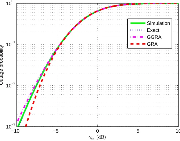
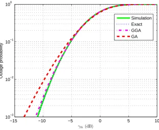
examined but with a simplified form. Fig. 1 and Fig. 2 show the OP vs. γth using EGC receivers
R= X11
X21+
X12X22
X32X42 which assumesL= 2and considering interferences while Fig. 2 describes the signal model as R =X11+X12X22+X13X23X33 which assumes L= 3 and does not consider
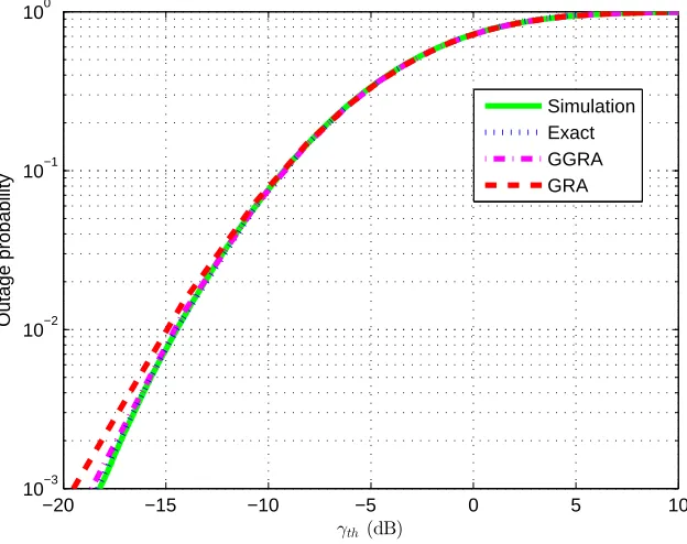
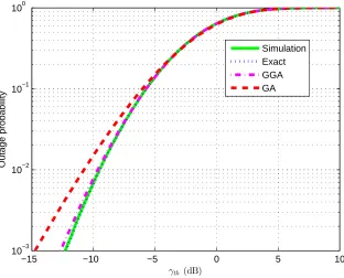
interferences. Fig. 3 and Fig. 4 show the OP vs. γth in multiple scattering channels, in which
Fig. 3 describes the signal model considering interferences as R= 2 X11
X21X31 + 3
X12X22X32
X42X52 while Fig. 4 describes the signal model without interferences as R=X11+ 2X12X22+ 3X13X23X33.
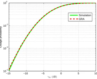
Moreover, Fig. 5 shows the OP vs. γth in terms of SIR in multiple scattering channel. In this
case, the SIR can be described as Iz =Z2, whereZ = X42+XX5211X+62X+21XX7231X82X92.
From Figs. 1 - 5, one can see that the OP increases when the SNR threshold increases, as
expected. In the extreme case when the SNR threshold goes to infinity, the OP will approach
one. Furthermore, the exact results of OP agree very well with the simulations in Figs. 1 - 4.
The approximate results based on GGRA match very well with simulations in Fig. 1 and Fig.
3 while GGA matches very well with simulations in Fig. 2 and Fig. 4, showing the usefulness
of our approximate expressions. The approximate result based on GRA matches well with the
simulations in Fig. 1 and Fig. 3 and GA matches well with the simulations in Fig. 2 and Fig.
4, both between 10−1 to 1 but with simple structures. Moreover, GRA has a very good match
with the simulation in Fig. 5.
V. CONCLUSIONS
The exact results of CDF of the sum of ratios of products and the sum of products of
independent α - µ RVs in the form of one-dimensional integral have been derived. Also, the
closed-form expressions for the CDF using GGRA, GRA, GGA and GA have been given.
Applications in obtaining the outage probability of EGC receivers for wireless multihop relaying
system considering interferences and without considering interferences have also been discussed.
Moreover, applications in obtaining the outage probability of signal transmitting in multiple
scattering channel considering interferences and without considering interferences are provided.
Numerical examples have shown the exact result derived agree very well with the simulations
GRA and GA have a considerable match in some cases but with a simple structure.
APPENDIX
A. Derivation of the PDF of Γ1,j
If α-µ RVs {Xjl} k,L
j=1,l=1 are independent, from [14] and using variable transformation, one
can get the PDF of Rl as
fRl(x) = Clx
−1α
l×
Gmn′′,m,n′′
tl
(
x ωl
)αl | 1−
µjl
mjl −
rl
mjl, rl = 0,1,· · · , mjl−1, j =m+ 1,· · · , k
µjl
mjl +
rl
mjl, rl = 0,1,· · · , mjl−1, j = 1,· · · , m
.
(11)
The moment generating function (MGF) of Rl is defined as MRl(s) =
∫∞
0 e
xsf
Rl(x)dx. With
the help of the Meijer’s G-function identity [15], [16, 07.34.22.0003.01], [16, 07.34.02.0004.01]
and [16, 07.34.02.0005.01], one can get MGF of Rl as (1).
B. Derivation of GGRA and GRA
One can see thatRis a sum of ratios of products. Therefore, we propose to use the ratio of GG
distribution to approximateR. Letx= r1
r2, wherer1 andr2 follow GG distribution with the PDFs of fr1(r;a1, d1, p) =
p a−d1 1 rd1−1e
−(r
a1)
p
Γ(d1
p)
, r > 0, and fr2(r;a2, d2, p) =
p a−d2 2 rd2−1e
−(r
a2)
p
Γ(d2
p)
, r > 0,
respectively. Then, one has the PDF ofxasfGGRA(x) =
∫∞
0 |r|f1(rx)f2(r)dr.After
simplifica-tion and using [17], one can getfGGRA(x) = pa−d1
1 a
d1
2 xd1−1(1+(
a2
a1)
pxp)−d1+pd2
B(d1
p,
d2
p)
.Usingk = (a1
a2)
p, one
can get the PDF of GGRA as (5). The CDF of GGRA is given byFGGRA(y) =
∫y
0 fGGRA(x)dx.
Using (5), the CDF expression above and with the help of [9, (3.259)], one can get the CDF of
GGRA as (6).
GRA have a simplified form which can be seen as the ratio of Gamma distribution. When
p= 1 infr1(r;a1, d1, p)andfr2(r;a2, d2, p), they become fr1(r;a1, d1) =
rd1−1e−r/a1
ad1 1 Γ(d1)
, r >0,and
fr2(r;a2, d2) =
rd2−1e−r/a2
ad2 2 Γ(d2)
, r >0,respectively. Similarly, usingfGRA(x) =
∫∞
0 |r|f1(rx)f2(r)dr
and k = a1
C. Moment-matching approximations
With the help of [17], one has the w-th order moment of GGRA as
E(XGGRAw ) = kw/pΓ(
d1
p + w p)
Γ(d1
p )
Γ(d2
p − w
p)
Γ(d2
p)
. (12)
Also, with the help of the [18], n-th order moment of R can be given as
E{Rn}=
n
∑
n1=0
n1 ∑
n2=0
· · ·
n∑L−2
nL−1=0 (n
n1 ) (n1
n2 )
· · ·(nL−2
nL−1 )
ωn−n1
1 ω
n1−n2
2 · · ·ω
nL−1
L m
∏
j=1
E{Xn−n1
j1 }
m
∏
j=1
E{Xn1−n2
j2 } · · ·
m
∏
j=1
E{XnL−1
jL } k
∏
j=m+1
E{ 1 Xn−n1
j1
}
k
∏
j=m+1
E{ 1 Xn1−n2
j2
} · · ·
k
∏
j=m+1
E{ 1 XnL−1
jL
}
(13)
where then-th order moment forXjlisE{Xjln}=
ˆ
γjlnΓ(µjl+n/αjl)
µn/γjljl Γ(µjl)
[8] and then-th order moment
for X1
jl is E{
1
Xn
jl}
= γˆjl−nΓ(µjl−n/αjl)
µ−jln/γjlΓ(µjl)
. Similarly, one can get the n-th order moment of P by
setting k = m and ignoring E{X1n
jl}
in (13) but they are omitted here to save space. Then d1,
d2, p and k in (5) and (6) can be determined by matching the 1-st, 2-nd, 3-rd and 4-th order
moment of R with the 1-st, 2-nd, 3-rd and 4-th order moment of GGRA, respectively as
E{R}=k1/pΓ(
d1
p+
1
p)
Γ(d1
p)
Γ(d2
p−
1
p)
Γ(d2
p)
E{R2}=k2/pΓ(
d1
p+
2
p)
Γ(d1
p)
Γ(d2
p−
2
p)
Γ(d2
p)
E{R3}=k3/pΓ(
d1
p+
3
p)
Γ(d1
p)
Γ(d2
p−
3
p)
Γ(d2
p)
E{R4}=k4/pΓ(
d1
p+
4
p)
Γ(d1
p)
Γ(d2
p−
4
p)
Γ(d2
p)
. (14)
Further, one can simplify (14) by getting rid of k as (7).
REFERENCES
[1] J. Zhao and G. Cao, “VADD: Vehicle-assisted data delivery in vehicular ad hoc networks,”IEEE Transactions on Vehicular
Technology, vol. 57, no. 3, pp. 1910–1922, May 2008.
[2] G. Karagiannidis, T. Tsiftsis, and R. Mallik, “Bounds for multihop relayed communications in Nakagami-mfading,”IEEE
Transactions on Communications, vol. 54, no. 1, pp. 18–22, 2006.
[3] G. Karagiannidis, N. Sagias, and P. Mathiopoulos, “N∗Nakagami: A novel stochastic model for cascaded fading channels,”
[4] N. Sagias, G. Karagiannidis, P. Mathiopoulos, and T. Tsiftsis, “On the performance analysis of equal-gain diversity receivers
over generalized gamma fading channels,”IEEE Transactions on Wireless Communications, vol. 5, no. 10, pp. 2967–2975,
2006.
[5] Y. Chen, G. Karagiannidis, H. Lu, and N. Cao, “Novel approximations to the statistics of products of independent random
variables and their applications in wireless communications,”IEEE Transactions on Vehicular Technology, vol. 61, no. 2,
pp. 443–454, 2012.
[6] D. Da Costa, M. Yacoub, and J. C. S. S. Filho, “Highly accurate closed-form approximations to the sum ofα-µvariates
and applications,”IEEE Transactions on Wireless Communications, vol. 7, no. 9, pp. 3301–3306, 2008.
[7] J. Salo, H. El-Sallabi, and P. Vainikainen, “Statistical analysis of the multiple scattering radio channel,”IEEE Transactions
on Antennas and Propagation, vol. 54, no. 11, pp. 3114–3124, 2006.
[8] M. Yacoub, “Theα- µdistribution: A physical fading model for the stacy distribution,”IEEE Transactions on Vehicular
Technology, vol. 56, no. 1, pp. 27–34, 2007.
[9] I. S. Gradshteyn and I. M. Ryzhik,Table of Integrals, Series, and Products, 7th ed. San Diego, CA: Academic, 2007.
[10] Y.-C. Ko, M.-S. Alouini, and M. K. Simon, “Outage probability of diversity systems over generalized fading channels,”
IEEE Transactions on Communications, vol. 48, no. 11, pp. 1783–1787, 2000.
[11] C. B. D and M. D. Springer, “The distribution of products, quotients and powers of independent H-function variates,”
SIAM J. Appl. Math., vol. 33, no. 4, pp. 542–558, 1977.
[12] S. Al-Ahmadi and H. Yanikomeroglu, “On the approximation of the generalized-K distribution by a gamma distribution
for modeling composite fading channels,” IEEE Transactions on Wireless Communications, vol. 9, no. 2, pp. 706–713,
Feb. 2010.
[13] S. Navidpour, M. Uysal, and M. Kavehrad, “BER performance of free-space optical transmission with spatial diversity,”
IEEE Transactions on Wireless Communications, vol. 6, no. 8, pp. 2813–2819, 2007.
[14] A. M. Mathai, “Products and ratios of generalized gamma variates,”Scandinavian Actuarial Journal, vol. 1972, no. 2, pp.
193–198, 1972.
[15] A. Prudnikov and O. Marichev, “The algorithm for calculating integrals of hypergeometric type functions and its realization
in reduce system,” inProc. of the international symposium on Symbolic and algebraic computation, 1990, pp. 212–224.
[16] The Wolfram Functions Site. http://functions.wolfram.com/NB/MeijerG.nb.
[17] C. A. Coelho and J. T. Mexia, “On the distribution of the product and ratio of independent generalized gamma-ratio
random variables,”The Indian Journal of Statistics, vol. 62, no. 11, pp. 221–255, 2007.
[18] J. C. S. S. Filho and M. D. Yacoub, “Nakagami-mapproximation to the sum of M non-identical independent nakagami-m
TABLE I
COMPARISON OF THE EXACT AND APPROXIMATEPDFS OFR= 2 X11
X21X31 + 3
X12X22X32
X42X52
x Exact GGRA GRA
3 0.005123366578 0.00553831 0.00657853
6 0.03437761985 0.0340766 0.0339683
9 0.05414392525 0.0538482 0.0528716
12 0.055066531 0.0550564 0.0544886
15 0.04670142108 0.0468074 0.0467473
18 0.03634886 0.0364498 0.0366334
21 0.027117528 0.0271797 0.0274094
24 0.019823972 0.0198519 0.0200418
27 0.014372777 0.014379 0.0145091
30 0.01040560788 0.0104009 0.0104784
33 0.007553075 0.00754393 0.0075832
36 0.00550956 0.00549977 0.00551409
39 0.0040442581 0.00403557 0.00403502
42 0.002989825 0.00298263 0.00297411
45 0.00222678 0.00222117 0.00220904
48 0.001670996 0.00166687 0.00165373
51 0.00126327 0.00126047 0.00124778
54 0.0009624243 0.00096032 0.000948797
57 0.0007384826 0.00073699 0.000726922
TABLE II
COMPARISON OF THE EXACT AND APPROXIMATECDFS OFR= 2 X11
X21X31+ 3
X12X22X32
X42X52
y Exact GGRA GRA
3 0.002918777902 0.00343157 0.00456575
6 0.05963044177 0.0603741 0.0635416
9 0.1977381439 0.197387 0.198466
12 0.3651634794 0.36438 0.363
15 0.5189965633 0.518401 0.516134
18 0.6435316511 0.643263 0.641246
21 0.7382844348 0.738262 0.736898
24 0.8082033983 0.808312 0.807589
27 0.8590801037 0.859235 0.858993
30 0.8959262807 0.89608 0.896146
33 0.9226282412 0.922759 0.922997
36 0.9420521725 0.942154 0.942469
39 0.9562621779 0.956336 0.956669
42 0.9667270005 0.966777 0.967096
45 0.9744897491 0.974522 0.974809
48 0.9802920019 0.980311 0.980559
51 0.9846609351 0.984671 0.98488
54 0.9879744607 0.987979 0.988152
57 0.9905062535 0.990509 0.990649
−10 −5 0 5 10 10−3
10−2 10−1 100
γth (dB)
Outage probability
[image:17.612.144.455.238.482.2]Simulation Exact GGRA GRA
Fig. 1. Outage probability vs. γth using EGC receivers in wireless multihop relaying system
−15 −10 −5 0 5 10 10−3
10−2 10−1 100
γth (dB)
Outage probability
[image:18.612.144.456.233.487.2]Simulation Exact GGA GA
Fig. 2. Outage probability vs. γth using EGC receivers in wireless multihop relaying system
−20 −15 −10 −5 0 5 10 10−3
10−2 10−1 100
γth (dB)
Outage probability
[image:19.612.144.456.249.496.2]Simulation Exact GGRA GRA
−15 −10 −5 0 5 10 10−3
10−2 10−1 100
γth (dB)
Outage probability
[image:20.612.144.456.245.497.2]Simulation Exact GGA GA
−15 −10 −5 0 5 10 10−3
10−2 10−1 100
γth (dB)
Outage probability
[image:21.612.144.456.232.487.2]Simulation GRA
Fig. 5. Outage probability vs. γth in terms of SIR in multiple scattering channel considering