Online Full Text



Abstract—Real-time inspection of glass substrates to detect defects has been very important because of the rapid growth in the flat panel industry. Since the wiring pitch of the glass substrate becomes increasingly narrower, it is difficult to detect defects from the time-series data obtained by the non-contact inspection machine because the data involves much noise. This study proposes machine learning-based methods of detecting defects in glass substrates with high precision in a short time. Several feature quantities are constructed not only to distinguish defects with noise but also to specify waveform types. In addition, numerical experiments are conducted using actual data to show the effectiveness of the proposed method.

Index Terms— Defect detection, Machine learning, Time-series data, Non-contact electric inspection, Glass substrate

I. INTRODUCTION

n recent years, the flat panel industry represented by liquid crystal, plasma, and organic electro-luminescence has been rapidly growing. In addition, the size of liquid crystal flat panels is increasing, and the definition is becoming higher. To increase the yield rate of products, it is important to check glass substrates in the midst of the production process. In the process, defects must be detected in a very short time. However, it is difficult to distinguish defects from noise in the inspected sensor data, because the wiring pitch is narrowed owing to the high definition of the glass substrate.

In automatic optical inspection (AOI) [11], inspected objects are scanned and compared with the standard image. Unfortunately, however, the AOI has some disadvantages with respect to the panel size to be inspected, alignment precision of the image, and sensitivity of lightning.

In this study, we focus on a non-contact electric inspection method in which glass substrates are inspected at high speeds without getting hurt, which has attracted attention in recent

R. Wakamatsu is with Department of Industrial Management Engineering, Graduate School of Engineering, Kanagawa University, 3-27-1 Rokkakubashi, Kanagawa-ku, Yokohama-shi, Kanagawa 221-8686, Japan (e-mail: [email protected]).

T. Uno is with Department of Mathematical Science, Graduate School of Technology, Industrial and Social Science, Tokushima University, 2-1, Minamijosanjima-cho, Tokushima-shi, Tokushima 770-8506, Japan (e-mail: [email protected]).

H. Katagiri is with Department of Industrial Management and Engineering, Faculty of Engineering, Kanagawa University, 3-27-1 Rokkakubashi, Kanagawa-ku, Yokohama-shi, Kanagawa 221-8686, Japan (phone: 045-481-5661; e-mail: [email protected]).

years. Hamori et al. [6] proposed a method of extracting only the waveform change in the defect by repeating the following three steps: (1) difference value calculation, (2) minute change emphasis, and (3) spike noise smoothing. Abeysundara et al. [1] considered an evolutionary optimized recurrent neural network for inspecting open and short defects on the line of a TFT and flat panel display (FPD).

Meanwhile, machine learning, which has attracted attention in recent years, is a framework which can be used for predicting and making judgments from the law of data by allowing computers to learn a large amount of data. Krummenacher et al. [8] proposed a method to detect and classify defective wheels using machine learning. In the detection, classifiers learn using a support vector machine which is a machine learning method, and the classification was learned and evaluated using a convolution neural network. In the research by Caesarendra et al. [2], the initial bearing defect was detected by combining the multivariate state estimation method and the successive probability ratio test from the feature quantity. Kernel regression was used to predict and estimate the useful life. Virupakshappa et al. [14] developed a new algorithm that uses features extracted from the output of the subband decomposition filter that incorporates support vector machines as a tool for classifying the presence or absence of defects in ultrasonic signals, and the accuracy was improved over the direct implementation without subband decomposition. Tabriz et al. [13] performed damage detection in rotating machines using empirical mode decomposition. They showed that the accuracy of damage detection was greatly improved by applying the amplitude calculation algorithm.

In this research, we consider a method to detect defects in glass substrates with high accuracy within the allowable time, using machine learning as a method to distinguish between defects and noise.

II. NON-CONTACT INSPECTION OF GLASS SUBSTRATE In the non-contact inspection of glass substrate [6], the wiring for driving the pixel of the flat panel is a conductor composed of Al or Ag. When the conductor is brought close to the position opposite to the conductor, an electrical capacity develops between both objects from the parallel- plate capacitor principle (refer to Figure 1).

Figure 1 Principle diagram of capacity coupling [6]

Machine Learning-based Methods for Detecting

Defects in Glass Substrate from Non-contact

Electrical Sensor Data

Ryota Wakamatsu, Takeshi Uno, Hideki Katagiri

Utilizing this principle, after receiving a micro voltage signal in a noncontact manner, analyzing the signal discriminates the presence or absence of wire disconnection and short circuit (refer to Figure 2).

Figure 2 System configuration diagram of noncontact inspection [6]

The minute voltage signal data are obtained by scanning over the wiring lines through the sensors of the noncontact inspection system. The voltage signal data are represented as time-series data (refer to Figure 3).

As shown in Fig. 3, the time-series data obtained from the sensors of the noncontact inspection system involve some noise. When a defect is present in the wiring line, the defect portion in a wave form has a remarkably different slope and amplitude as compared with the peripheral portion. Therefore, the most basic idea to detect defects is to set an appropriate threshold value as shown in Fig. 3. However, an appropriate threshold value is difficult to set because of some reasons.

Figure 3 Waveform data obtained from a non-contact inspection machine through electric sensors

One of the reasons for the difficulty in setting an appropriate threshold value stems from the existence of noise and the non-stationarity of the waveform. In Figure 4, a change point of a defect is shown, whereas the left part represents noise. The threshold value in Fig. 4 does not work well because noise is recognized as defects. Therefore, an efficient algorithm for distinguishing between defects and noise is necessary.

Figure 4 Non-stationarity of the waveform

Many studies have been conducted on defect detection algorithms based on signal processing techniques such as the fast Fourier transform (FFT) and wavelet transform. Unfortunately, these studies cannot be directly applied to our problem because FFT and wavelet transform need more computational time than the perceptional time in this study.

Hamori et al. [1] proposed a method of extracting only the

waveform change in the defect part by repeating three steps: (1) difference value calculation, (2) minute change emphasis, and (3) spike noise smoothing. The method is fast and practical; however, three problems need to be resolved. The first problem is that false detection frequently occurs for some types of waveforms. The second one is that it is difficult for the algorithm to detect minute defects that have small change points. The last one is the difficulty in manually setting an appropriate threshold value.

Abeysundara et al. [2] considered an evolutionary optimized recurrent neural network for inspecting open and short defects on the line of a TFT and FPD. The defect detection accuracy is improved, but it can be applied only for some specific cases.

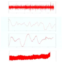
These two previous studies did not consider the "diversity of waveforms" as shown in Figure 5. Because many types of glass substrates are to be inspected, a large variety of time-series waveform data is obtained from the non-contact inspection machine.

Figure 5 Various types of waveform

This study provides some machine learning-based defect detection algorithms. In machine learning, it is important to construct the appropriate feature quantities. The following section provides five feature quantities not only to discriminate the defects with noise but also to cope with the waveform diversity.

III. PROPOSED METHOD A. Feature quantity

waveform diversity is difficult to cope by only the Z score and isolation degree; the defect-noise discrimination judgment differs depending on the waveform type.

To consider the waveform characteristics, three other feature quantities such as the trend rate, average number between extreme points, and variation rate are useful. Feature amount to distinguish between defects and noise

First, to judge the presence or absence of a trend, the trend degree, represented by Tr, is introduced.

Tr = (Mmax － Mmin)(Dmax － Dmin) (1)

where M represents the moving average curve (baseline) and D represents the original data, focusing on the respective maximum and minimum values. If Tr is larger than the threshold value, the existence of a trend is assumed. Subsequently, the trend removal process is performed by subtracting a moving average curve from its original data. The obtained moving average curves are dependent on the length of the moving average periods (MAPs). In this study, we calculate the MAP based on two features: (1) the average number of points between extreme points, and (2) the ratio of the number of extreme points to the number of all points. More specifically, we calculate the MAP as follows:

(2)

where x is the average number of data between polar points, y is the ration of the number of maximum or minimum points, and (a,b,c) is a set of parameters.

The algorithm of calculating the Z score and isolation degree is as follows:

Step 1. Set the values of parameters a,b and c in Equation (2), and calculate the moving average periods MAP(x,y).

Step 2. Calculate the moving average curve (baseline) for data using MAP(x, y) (refer to Figure 6).

Figure 6 Calculation of moving average curve

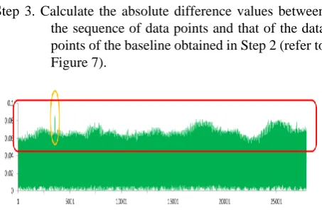
Step 3. Calculate the absolute difference values between the sequence of data points and that of the data points of the baseline obtained in Step 2 (refer to Figure 7).

Figure 7 Absolute difference values between the sequence of data points and its baseline

Step 4. Calculate the trend degree of data points obtained in Step 3 using Equation (1). If the trend degree Tr> α, extract the data points corresponding to the maximum value (refer to Figure 8).

Figure 8 Extraction of local maximum points

Step 5. Let Up be the number of data points obtained in Step 4. If Up > MAP(x, y), return to Step 1.

Step 6. Calculate Z score denoted by Equation (3) and isolation degree denoted by Equation (4).

(3)

(4)

where is the th amplitude in the time window width, and is the amplitude magnitude of the upper in the interval. is the amplitude corresponding to the th extreme point, is the average value of extreme points excluding the top five points, and σ is the standard deviation. Data points corresponding to defects tend to have abrupt changes with large amplitudes. The Z score calculated by Equation (3) represents the degree of magnitude.

Nevertheless, a sequence of data points with large amplitudes is considered as noise. The isolation degree expressed in Equation (4) is introduced because the data points corresponding to defects, called a defect point, tend to be isolated. In other words, the amplitude of the data points near the defect points is by far smaller than the amplitude of the defect point.

Feature quantities for specifying waveform types

This section provides three feature quantities for specifying the types of waveforms: (1) trend degree, (2) average number between extreme points, and (3) vibration degree.

The first feature quantity is a trend degree denoted by Equation (1), which represents the magnitude of the wave trend and is expressed using Equation (1).

The second one is the average number between extreme points that represents the severity of vibration and is expressed by Equation (5).

= (5)

where ci is the number of points between the ith extremal

The variation rate represents the variance of the amplitude and is expressed by Equation (6).

A＝ (6)

where and are defined as

＝

(7)

＝

(8) Si is the difference between the ith extreme point and

(i+1)th extreme point, and is the average of the absolute values of the differences between the extreme points.

B. Over-sampling

When there exists a considerably large difference between the amount of major-class data and that of the minor-class data, over-learning or over-fitting often occurs. For example, if a learning model is constructed using unbalanced data in which the amount of normal data is by far larger than that of the abnormal data, then the results predicted by the method are always normal. To avoid such an over-learning problem, we use an over-sampling method called synthetic minority over-sampling technique (SMOTE), which was proposed by Chawla et al. [3]. Instead of duplicating the selected specimen, based on the k-nearest neighborhoods of the selected specimen, the SMOTE synthesizes new samples and increases the number of samples, which transforms unbalanced data into balanced data.

C. Defect detection by machine learning techniques Using the five feature quantities proposed in the previous section, we construct machine learning-based models for detecting defects in the glass substrate through the time-series data of voltage obtained from the sensors of the non-contact inspection machines. More specifically, we examine the k-nearest neighbor (k-NN) algorithm, support vector machine [12], random forest [9], and gradient boosting [5].

In the k-NN algorithm, the nearest k-data points to each data point is taken into consideration. For each data point, the numbers of normal data points and abnormal data points are counted and compared, and the class of each data point is classified as normal or abnormal, based on the larger number of data points among the k nearest neighborhoods.

The support vector machine is used for classification and discrimination by calculating a hyperplane that maximizes the distance from the normal data points and abnormal data points.

Random forest is a method that uses a set of decision trees in which the conditional branching of feature quantities together with majority voting are performed for classification and discrimination.

Gradient boosting is a method of generating models that are better than those in the previous step by updating a set of learning data. Learning data updating is performed by adding some new data to the learning data in the previous step to lessen the difference between the result obtained from the current learning data and the objective value.

IV. EXPERIMENTAL RESULTS

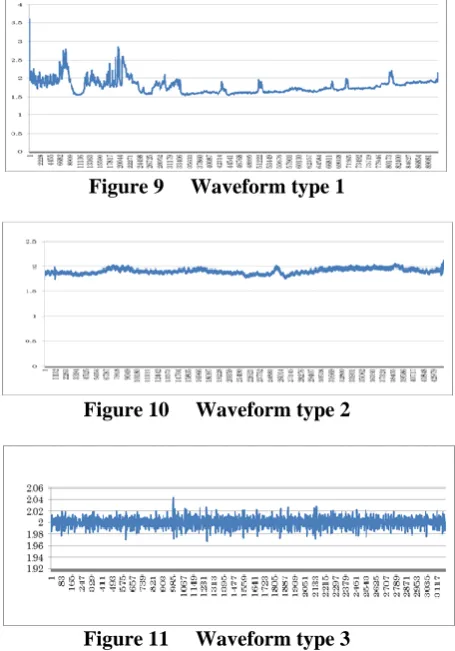
To confirm the effectiveness of the proposed methods, we conduct numerical experiments using real data. In the experiments, we used three types of time-series data corresponding to three different types of glass substrates, which are obtained by sensing the voltage via a non-contact inspection machine, as shown in Figures 9-11．Based on our preliminary experiments, the values of parameters a, b, c in Equation (2) are determined as 0.3, , 110, respectively.

Figure 9 Waveform type 1

Figure 10 Waveform type 2

Figure 11 Waveform type 3

As for the machine learning platform tools, we used the R language together with the packages of class kernlab, randomForest, and XGboost. The version of R language we used was R 3.4.3. Further kernlab [7] is an SVM package based on the kernel method used as a classification method, which can specify the parameters of the kernel functions; randomForest [10] is a package that performs optimal classification and computes the optimum number of decision trees and its estimated error rate; XGboost [4] is a scalable, end-to-end gradient boosting method that can process millions of samples using off-core calculations and has far less information volume to achieve more than billions of extensions. The parameters are manually set using the k-NN algorithm and support vector machine, whereas the parameters of random forest and gradient boosting methods are set with the default values of the packages.

To compare and evaluate the performance of the machine learning-based methods, we used four evaluation criteria: (1) accuracy, (2) true positive rate (TPR), (3) true negative rate (TNR), and (4) precision.

involving three types of waveforms. We divided the data into two sets: (1) data for learning models, and (2) data for predicting whether each data point is a defect or noise.

A. Learning data involving a single type waveform

First, we conducted experiments using the data involving a single-type waveform when the k-NN algorithm is used. Tables 1 to 3 show the experimental results in which the learning data involve only one type of waveform, namely, waveform types 1, 2, and 3, respectively.

Table 1 Results for type 1 (k-NN: single)

k-NN(k=1) k-NN(k=10) k-NN(k=20)

Accuracy 0.998 0.998 0.994

TPR 0.998 0.998 0.994

TNR 1.000 1.000 1.000

Precision 1.000 1.000 1.000

Table 2 Results for type 2 (k-NN: single)

k-NN(k=1) k-NN(k=3) k-NN(k=5)

Accuracy 0.999 0.999 0.999

TPR 0.999 0.999 0.999

TNR 1.000 1.000 1.000

Precision 1.000 1.000 1.000

Table 3 Results for type 3 (k-NN: single)

k-NN(k=1) k-NN(k=3) k-NN(k=5)

Accuracy 0.996 0.998 0.996

TPR 0.998 1.000 0.998

TNR 0.900 0.909 0.900

Precision 0.998 0.998 0.998

Tables 1 to 3 show that the performance of the k-NN algorithm is dependent on the k values. Further, the best k values are dependent on waveform types. The k-NN algorithm appears difficult to apply to our problem.

Next, we conducted the experiments using the support vector machine (SVM), random forest (RF), and gradient boosting methods (XGB). Tables 4 to 6 show the experimental results in which the learning data involve only one waveform type (waveforms 1, 2, and 3, respectively).

Table 4 Results for type 1 (SVM, RF, XGB: single) SVM

=0.001

Random Forest

XG Boost

Accuracy 0.998 0.975 0.975

TPR 0.998 0.974 0.974

TNR 1.000 1.000 1.000

Precision 1.000 1.000 1.000

Table 5 Results for type 2 (SVM, RF, XGB: single) SVM

= 0.01

Random Forest

XG Boost

Accuracy 1.000 0.999 0.999

TPR 1.000 0.999 0.999

TNR 1.000 1.000 1.000

Precision 1.000 1.000 1.000

Table 6 Results for type 3 (SVM, RF, XGB: single) SVM

=1.0

Random Forest

XG Boost

Accuracy 0.994 0.990 0.983

TPR 1.000 0.990 0.982

TNR 0.769 1.000 1.000

Precision 0.994 1.000 1.000

Tables 4 to 6 show that the support vector machine is the best among the three methods.

B. Learning data involving multiple waveform types In this section, we show the experimental results in which the learning data involve multiple waveform types. When the waveform type is unknown, the models should be learned using all possible waveform types. In each experiment, the learning data involve three types of waveforms (waveform type 1, waveform type 2, and waveform type 3), whereas the evaluation data involve a single type of waveform.

Tables 7 to 9 show the experimental results of the k-NN algorithm in which the evaluation data in each experiment involves a single type of waveform, namely, waveform types 1, 2, and 3, respectively.

Table 7 Results for type 1 (k-NN: multiple)

k-NN(k=10) k-NN(k=20) k-NN(k=80)

Accuracy 0.998 0.998 0.994

TPR 0.984 0.984 0.994

TNR 1.000 1.000 1.000

Precision 1.000 1.000 1.000

Table 8 Results for type 2 (k-NN: multiple)

k-NN(k=1) k-NN(k=2) k-NN(k=5)

Accuracy 1.000 0.999 0.999

TPR 1.000 1.000 1.000

TNR 1.000 0.714 0.625

Precision 1.000 0.999 0.999

Table 9 Results for type 3 (k-NN: multiple)

k-NN(k=1) k-NN(k=3) k-NN(k=5)

Accuracy 1.000 0.996 0.994

TPR 1.000 0.998 0.996

TNR 1.000 0.900 0.889

Precision 1.000 0.998 0.998

Similar to Tables 1 to 3, Tables 7 to 9 show that the performance of the k-NN algorithm is dependent on the k values. Further, the best k value is dependent on the waveform type. The k-NN algorithm appears difficult to apply to our problem.

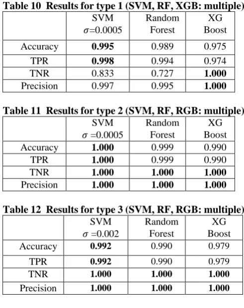
Table 10 Results for type 1 (SVM, RF, XGB: multiple) SVM

=0.0005

Random Forest

XG Boost

Accuracy 0.995 0.989 0.975

TPR 0.998 0.994 0.974

TNR 0.833 0.727 1.000

Precision 0.997 0.995 1.000

Table 11 Results for type 2 (SVM, RF, RGB: multiple) SVM

=0.0005

Random Forest

XG Boost

Accuracy 1.000 0.999 0.990

TPR 1.000 0.999 0.990

TNR 1.000 1.000 1.000

Precision 1.000 1.000 1.000

Table 12 Results for type 3 (SVM, RF, RGB: multiple) SVM

=0.002

Random Forest

XG Boost

Accuracy 0.992 0.990 0.979

TPR 0.992 0.990 0.979 TNR 1.000 1.000 1.000

Precision 1.000 1.000 1.000

Table 10 shows that the support vector machine and XGboost are competitive for waveform type 1. Because the TNR of the support vector machine is 0.833, which is very low, we concluded that XGboost is the best for waveform type 1. As for waveform types 2 and 3, the support vector machine is the best among the three methods.

V. CONCLUSION

In this research, we provided machine learning-based methods of detecting defects in glass substrates by analyzing time-series data obtained from a non-contact inspection method. We proposed several feature quantities that are useful to discriminate between defects and noise. Using the proposed feature quantities, we conducted some numerical experiments and compared the performances of the representative machine learning techniques such as the k-nearest neighbor algorithm, support vector machine, random forest, and gradient boosting. Our experimental results show that the support vector machine has higher prediction accuracy than the other methods.

As future work, we will conduct more experiments to show the effectiveness of the proposed methods because many types of waveforms are available. Another future work is to focus on other machine learning and/or statistic analytical methods such as recurrent neural network, density ratio estimation, subspace method, and deep learning.

ACKNOWLEDGMENTS

We would like to thank Dr. Hiroshi Hamori, President and Representative Director of OHT Co., Ltd. for providing the glass substrate inspection data.

REFERENCES

[1] H. A. Abeysundara, H. Hamori , T. Matsui, M. Sakawa, Defects detection of tft lines of flat panel displays using an evolutionary optimized recurrent neural network, American Journal of Operations Research 4 (3), 2014, pp.113-123

[2] W. Caesarendra, T. Tjahjowidodo, B. Kosasih, A. K. Tieu, Integrated condition monitoring and prognosis method for incipient defect detection and remaining life prediction of low speed slew bearings, Machines-Open Access Engineering Journal 5 (2), 2017, pp.1-20 [3] N. V. Chawla, K. W. Bowyer, L. O. Hall, W. P. Kegelmeyer, SMOTE:

Synthetic Minority Over-sampling Technique, Journal of Artificial Intelligence Research 16, 2002, pp.321-357

[4] T. Chen, C. Guestrin,Xgboost: a scalable tree boosting system, KDD '16 Proceedings of the 22nd ACM SIGKDD International Conference on Knowledge Discovery and Data Mining, 2016, pp.785-794 [5] J. H. Friedman, Stochastic gradient boosting, Computational Statistics

& Data Analysis 38 (4), 2002, pp.367-378

[6] H. Hamori, M. Sakawa, H. Katagiri, T. Matsui, Fast non-contact flat panel inspection through a dual channel measurement system, Proceedings of the 40th International Conference on Computers & Indutrial Engineering, 2010, pp.1-6

[7] A. Karatzoglou, A. Smola, K. Hornik, A. Zeileis, kernlab - An S4 Package for Kernel Methods in R, Journal of Statistical Software 11 (9), pp.1 - 20

[8] G. Krummenacher, C. S. Ong, S. Koller, S. Kobayashi, J. M. Buhmann, Wheel defect detection with machine learning, IEEE Transportation On Intelligent Transportation Systems, 2017, pp.1-12

[9] R. L. Lawrence, S. D. Wood, R. L. Sheley, Mapping invasive plants using hyperspectral imagery and breiman cutler classifications (randomforest), Remote Sensing of Environment 100(3), 2006, pp.356-362

[10] A. Liaw, M. Wiener, Classification and Regression by randomForest, The Newsletter of the R Project 2 (3), 2002, pp.18-22

[11] H. Rau, C. H. Wu, Automatic optical inspection for detecting defects on printed circuit board inner layers, International Journal of Advanced Manufactring Technology 25 (9), 2005, pp.940-946

[12] J. A. K. Suykens, J. Vandewalle, Least squares support vector machine classifiers, Neural Processing Letters 9 (3), 1999, pp.293-300 [13] A. A. Tabrizi, L. Garibaldi, A. Fasana, S. Marchesiello, Performance