Forecasting conditional volatility on the RIN market using MS GARCH model

Munich Personal RePEc Archive

Forecasting conditional volatility on the

RIN market using MS GARCH model

Kakorina, Ekaterina

European University at Saint-Petersburg

July 2014

Online at https://mpra.ub.uni-muenchen.de/56704/

FORECASTING CONDITIONAL VOLATILITY ON THE RIN MARKET

USING MS GARCH MODEL

Ekaterina Kakorina

European University at Saint-Petersburg

[email protected]

Contents

Introduction ... 2

1. The market description ... 5

1.1. What does RIN mean? ... 5

1.2. The main actors of the market ... 6

1.3. The last market tendency ... 9

2. Theoretical background ... 11

2.1. Description of models which are useful for forecast ... 11

2.2. Description of the chosen model ... 14

2.3. Preparation tests ... 17

2.4. One-sample Kolmogorov-Smirnov test ... 18

2.5. Forecast volatility and returns ... 20

3. Results of estimation ... 22

3.1. Data description ... 22

3.2. Test results ... 23

3.3. Returns description ... 25

3.4. Results of estimation ... 26

3.5. Results of forecast ... 29

3.6. Comparing the price forecast with the forecast doing by EPA ... 30

Conclusion ... 32

Bibliography ... 34

Appendix ... 39

2

Introduction

In the recent years the topic about pollution of environment is quite popular.

Many countries organize the government policy taking into account

environmentally friendly policy. Dealing with pollution problems is one of the

wide-spread sphere of using Pigovian tax. It is considered that this tax allows

decreasing level of emissions with the least public costs.

According to the idea which was offered by A. Pigou, appearance of

externalities means the difference in estimations economical situation from two

points of view. On the one hand, it is private which includes only interests of

participants of a concrete business. On the other hand, it is social or public which

allow for interests of all economic units including third party.

So both types of externalities lead to market inconsistence in effective

distribution of resources. For going back to effective stage it is necessary to

implement internalization or change externalities to internal effects. So if this

method is created and difference between private and public estimations

disappears, all economic units will include externalities in their estimation. There

are two ways to solve problems of externalities, the first one is using possibilities

of private sector and the second way is using government possibilities.

From the government side it is possible to use different cash payments

(taxes) or regulation. In the first case necessity to make payment, which was

established by the state, corrects private costs and benefits regarding to public ones

and parties make effective decisions. In the second case government can influence

economic units strongly through system of administrative and legal methods.

However, the combination of these two cases is possible too, and an

example of it can be the world emission market which is closely linked to the

Kyoto Protocol. The market based emissions trading schemes and carbon taxes.

The emission trading is market-based approach used to control pollution by

providing economic incentives for achieving reductions in the emissions of

3

other commodities markets, are that it is a politically-generated and managed

market and that the underlying is a dematerialised allowance certificate, as

opposed to a physical commodity [1.16]. A broad range of countries have

introduced this market such as China, Japan, European countries and the USA.

According to statistics presented by Department of the Environment of

Australian government [2.2], the USA has 18.3% of Global Emissions including

residential and commercial buildings. It is the second place in the world rating of

counties’ pollution. Only three countries have percentage which is higher than

10%. The first place is China and the third one is the European Union which have

19.1% and 13.4% respectively.

Maybe because of big share of the world pollution the USA organized not

only the emission market, but also the RIN market. The RIN market plays a critical

role in successfully implementing the RFS2 (Renewable Fuel Standard) which was

introduced after enactment of Energy Policy Act of 2005 [1.29].

The emergence of this market is connected with partial transition from

traditional fossil fuels to a more environment fuels as renewable ones or ethanol,

which is obtained by processing of corn, cereals, cellulose or others. So drivers

used not clear gasoline, but mixture of gasoline and ethanol in some proportion.

Moreover, the RIN market has the trading system too, actors can trade

securities as RINs. There are several limitations, firstly, each blender should have

concrete number of RINs at the reporting period at the end of year, and secondly,

after two years of RIN existence the security loses all functions.

Besides that, many researches drew attention to the RIN market after the

huge increase of price of one RIN at the end of 2012. At the same time there was

change of trend. It was one of the popular issue under discussion, in the other

words, scientists and workers tried to understand what happened and what

influenced RIN prices. Nowadays there is a less developed set of risk management

tools, compared to other markets, for firms active even in the emissions markets,

4

[1.16]. It influences not only investigation of the emission market, but also the RIN

market, since they are similar.

To address these problems we need to find process which explained price

behavior and forecast conditional volatility and returns.

This paper consists of four sections. Section 1 describes the RIN market,

defines RIN, specifies key actors and their functions as well as functions of EPA,

which controls the market performance, and the last changes on the market.

Section 2 includes information about some possible models to estimate RIN prices.

Section 3 illustrates all results which were achieved. The last section is conclusion,

which repeats main characteristics of the market and all results of estimation and

5

1. _{The market description}

1.1. What does RIN mean?

Regarding RFS, which is standard set based Energy Independence and

Security Act of 2007, every gallon of renewable fuel has to be identified in the

system of accounting units of renewable fuels and to have unique renewable

identification number (RIN). Additionally, RIN has to be given not only to every

gallon of ethanol which was produced in the USA, but also to every gallon of

imported ethanol. So this way the government stimulates blenders to add ethanol to

gasoline before selling it to the service stations.

According to Security Act of 2007, US Environmental Protection Agency

(EPA) establishes requirements for the production, transportation and export of

renewable fuels. Due to the predominance of ethanol obtained from corn

(conventional ethanol), the most common RIN is for this kind of biofuel

(conventional RIN). Moreover, EPA establishes mandate for every blender, it

means that each of them must have more than the concrete number of RINs at the

reporting period at the end of year. If blender has deficit or surplus of RINs, they

can buy or sell RINs separately from ethanol. Blenders communicate with each

other strongly or through special agencies, because nowadays RIN is not traded on

the Exchange. [1.19]

RIN is a 38-digit serial number had unique code of biomass gallon, number

of consignment, producer and type of biofuel (conventional, advanced or others).

Depending on the type of biofuel RIN is called conventional, cellulosic, biodiesel

or others (Fig. 1). In addition to that, RIN is security, because it is a financial

instrument that represents an ownership position in a publicly-traded corporation,

and tax, because every blender has to pay it and control level of pollution.

Also RIN is investment as emissions. “A key aspect of EU scheme [trading

scheme of emissions] is that it allows companies to use credits from Kyoto’s

project-based mechanism, joint implementation and the clean-development

6

means the system not only provides a cost-effective means for EU-based industries

to cut their emissions but also creates additional incentives for businesses to invest

in emissions-reduction projects in developing nations as China and India, and in

South America and Africa.” [1.17] So RIN is instrument which reallocates cash flows from blenders of one state to blenders of other states.

Figure 1. Renewable Identification Number code definitions [1.28]

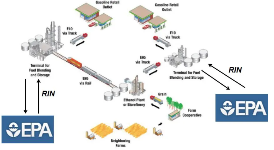
1.2. The main actors of the market

All actors of the RIN market can be divided into following groups (Fig.2):

1. Farmers;

Farmers are entrepreneurs who grow raw materials for ethanol. As it was

mentioned before, it may be corn, grain crops or other agricultures. This group is

also included entrepreneurs who prepare wood for processing (ethanol production).

2. Refiners;

Refiners are manufactures who produce ethanol. The number of refiners is

about 211 in 28 states, common productivity is approximately 14.7 bln gallons of

7

decrease. In 2005 production surged because of imposition of RFS. This increase

was not only because of production rise in old plants, but also because of building

new ones. For 10 years the number of plants becomes fourfold and the number of

states has already increased by 40%. [2.7]

3. Blenders;

Blenders are manufactures who mix ethanol with gasoline. It must be

mentioned that blenders are located not in the same places as refiners. Blenders are

concentrated in the Northern or North-Western parts of the USA, but refiners are

generally placed on coasts. The latter can be explainable by necessity to import or

export gasoline and ethanol.

4. Owners of fuel stations;

This group includes entrepreneurs who sell fuel to ultimate consumers. Their

number depends on fuels what they sell. For example, E85 were sold by 3000

fueling stations. It was because of the number of vehicles which fuel was for.

In the end of 2010 EPA allowed to use E15, but only for vehicles which

were produced after 2001. In spite of better properties than E10, E15 were less

popular. In 2011 only 10 fueling stations sold it. However, in 2013 there were

about 24 fueling stations selling E15 out of 180,000 stations across the U.S. [2.3]

According to information presented by Department of Energy, there are 10 mln of

FFVs1 in the USA and only 500 thousand of them are filled up E85. One of

reasons is that owners do not know about characteristics of their cars [2.4].

5. EPA;

This actor regulates the market. In other words, every year it checks that

every gallon of ethanol, which is produced in the USA or imported to the country,

has RIN and every blender has enough RIN, not more that 20% are transited to

next year and there are other violations. Also it analyzes current situation to

forecast the value of mandate for next year. Forecast is really responsible thing,

because, as it will be mentioned below, some researchers argue that it can

influence RIN prices.

8

All work of this agency is addressed to reducing carbon pollution and other

greenhouse gas emissions from the transportation and energy sectors. In

collaboration with other agencies which work, EPA will build strong partnerships

with states, tribes, and local communities to enhance the resiliency of local

infrastructure as part of EPA's Sustainable Communities initiative. [2.5]

6. Private agencies

Private agencies provide information about RIN prices, the market review.

Examples of them are RINAlliance2 and EcoEngineers3.

Renewable fuel blenders across the country utilize the experience of

regulatory professionals as private agencies for consulting, compliance, RIN

management and RIN marketing services as well as other services in the renewable

fuel sector including plant design review, compliance advisory, on-site verification

and certification and regulatory consulting under national and international

renewable fuel standards.[2.9]

Figure 2. Scheme of the RIN market**write mandate, move RIN and arrows

Nowadays RINAlliance is one of the biggest private agencies in the USA

which serves 130 blenders with EPA reporting and RIN marketing. They currently

2

http://rinalliance.com/

3

9

manage more than 2 million RINs per day while aggregating and marketing RINs

that have been separated within the RINAlliance system. Because of 140 million

fraudulent RINs circulating within the RFS RIN system RINAlliance and other

agencies had to design a new system of due diligence that was capable of

re-establishing the relationships between RIN buyers and sellers.

Since 2011 RINAlliance has been partnering with EcoEngineers to design a

third party assurance plan that provided on-site audits and continual monitoring of

feedstock, production, fuel quality, and overall mass-balance of facilities. EPA is

currently drafting rules that promote a similar process (RIN Quality Assurance

Program) for the identical reason of making the RIN market stable. [1.17]

1.3. The last market tendency

Since the end of 2013 researchers have started to have interests in behavior

of RIN prices and efficiency of the market. For example, an analysis by Iowa State

University economists B. Babcock and S. Pouliot of the EPA's ethanol market

system finds that it works effectively and as intended in tracking compliance with

RFS. The authors conclude that rather than volatility and high prices which were at

the end of 2012 being a sign that something was wrong with RIN markets or RFS,

RIN prices did their job by signaling that higher ethanol mandates were coming

and would be costly to achieve. [2.8] This huge ‘jump” of the price can be because

of reducing the size of the corn crop and that led to record-high prices and the

idling of ethanol plants in late 2012 and early 2013, as market prices for ethanol

were not sufficient to allow producers to offset higher production costs and sustain

significantly positive margins. [2.1]

Some scientists researched thе dependence between mandate and price level.

For example, R. Miao and et al. [1.30] develop a two-period conceptual model.

They find that the investment impact of mandates depends on investors’ marginal

10

In the summer of 2013 there was significant price increase of three assets at

the same time. Firstly, gasoline and RIN prices grew, and then gas prices went up.

Some experts conjectured that the financial crisis would repeat. However, the

Renewable Fuels Association concluded that it was seasonal driving and influence

of rising of crude oil price as well as that, according to results of Granger causality

analysis, there is no causality between gasoline and RIN prices. [2.1]

At the end of 2013 EPA determined biofuel mandate levels for 2014 which

became hither. Babcock and Pouliot argue this increase will lead to fall of RIN

prices dramatically. Because high RIN prices imply high compliance costs, this

mandate would create a large incentive to lower compliance costs. [1.2]

All these factors influence RIN prices, but now it is impossible to understand

all impacts. As executive director of media relations for Valero Bill Day

mentioned, “it is difficult to analyze the RIN market <…> because the RINs

market is so opaque. It’s not a regulated market like gasoline or crude oil or other

commodities that trade on the New York exchange or CBOT. It’s mostly private

transactions.” [2.6]

This paper is just an attempt to understand behavior of RIN prices and

forecast their value. It does not present other factors which can influence RIN

11

2. _{Theoretical background}

2.1. Description of models which are useful for forecast

In this section we describe models which are useful for forecast when a

researcher has only one series without any other factors which can explain

behavior of given variable. These models are ARMA, ARMA-GARCH,

GARCH-M and GARCH-MS ARGARCH-MA-GARCH.

ARMA

One of the key moments in Econometrician history was in 1951 when Peter

Whittle published his thesis which described autoregressive–moving-average

(ARMA) model. [1.39] Since this year many of authors used the model to analyze

time series and forecast future values of series. For example, using ARMA model

it is possible to forecast births as J. McDonald do. [1.28] Additionally, N. Muler

and et. al deal with inward movement of residential telephone extensions in a fixed

geographic area. [1.31]

The model consists of only equation:

where a given time series, c is a constant, are parameters of the

autoregressive part, are parameters of the moving average part and

are white noise error terms. Because of the number of parameters, it is

usually called ARMA(p,q).

This model is useful, but it works only with stationary time series whereas

many of them have integrability of order one or two. In other words, if author

analyzes price dynamics which is non-stationary and has time series integrability

of order one then returns will be stationary, but it will ARIMA(p,1,q) model.

Besides existence of unit roots, conditions of statinarity for AR should be

12

should be more than one in absolute value. In the case of AR(1), it is -1< <1.

MA is always stationary.

ARMA-GARCH

Financial data usually estimated using ARMA-GARCH models which have

not only ARMA equation, but additional one described behavior of volatility. For

example, A. Carvalhal and B. Mendes estimated usual ARMA-GARCH model

working with emerging market stock returns. 1.6] Also there are some

modifications such as FIGARCH, which was estimated by K. Choi and S.

Hammoudeh [1.5] who deal with the spot and futures prices of crude oil and of two

refined products such as the gasoline and heating oil, or ARMA-EGARCH, which

was estimated by M. Karanasos and J. Kim who research four East Asia Stock

Indices. [1.20]

ARMA(p,q)-GARCH(k,m) model has the following structure:

where a given time series, c and are constants, are

parameters of the autoregressive part, are parameters of the moving

average part, are residuals; and are parameters of

GARCH model, is conditional heteroskedasticity as well as is white noise

with standard normal distribution.

This model was described by Bollerslev (1986) [1.29]. If heteroskedasticity

depends on only errors, it is ARCH model which was offered by Engle (1982)

13

As ARMA model, GARCH also has some restrictions. First of all, the

unconditional variance

is not negative, so

, where . Secondly, for (weakly) covariance stationary of

the process the roots of the equation

have to be outside unit circle. Lastly, should be positive, but and

should be not negative for all i and j.

GARCH-M

The return of the asset can depends not only on previous returns of different

periods (AR model) and residuals of previous periods (MA model), but also on its

volatility (GARCH-M or GARCH in Mean). In other words, the

ARMA(p,q)-GARCH-M(k,m) model has the following structure:

The parameter does not any limitations, but the sign of this parameters shows

that the return is positively or negatively related to volatility.

MS GARCH

In recent years researchers of financial assets have started to work with MS

GARCH which was suggested by Hamilton (1989) [1.13]. The idea of this model

is that parameters dependent from two or more regimes.

There are two types of this model. The first one is path-dependent MS

GARCH model, the conditional density of depends on all previous values of .

It complicates the model estimation, because of the number of parameters which

increases period by period, so authors use Monte Carlo method. For instance, L.

14

and J.Henneke estimated MS-ARMA-GARCH model using the stock price series

which is the value-weighted portfolio of stocks traded on the NYSE [1.15].

The second type is non- path-dependent MS GARCH model of Klassen

[1.23], the conditional density of depends only on the current regime . The

number of parameters is the same for all periods, so authors use maximum

likelihood method. For example, S. Blazsek and A. Downarowicz estimated hedge

fund indices and forecast volatility [1.4], J. Marcucci analyzes closing price index

from the S&P100 stock market [1.26].

According to results of White’s Reality Check test [1.41] and Hansen’s test [1.14] for Superior Predictive Ability which were compared by Marcucci [1.26],

the MS GARCH model with normal innovations does outperform all standard

GARCH models in forecasting volatility at shorter horizons. At longer horizon,

standard GARCH models outperform the MS GARCH.

MS GARCH model also has three equations as GARCH:

where is a regime which forms a Markov process.

2.2. Description of the chosen model

In this paper we illustrate non-path-dependent MS AR(1)-GARCH-M(1,1)

model with two regimes for normal and Student-t distributions. The main idea of

using MS GARCH is to forecast zero returns which can’t be forecasted by

GARCH model and, on the other hand, it is not correct to exclude them as some

authors did, for example, in a paper where O. Sabbaghi and N. Sabbaghi research

15

discussed in the paper by M. Paolella and L. Taschini [1.32] and authors suggest

two ways. The first way is to do only the unconditional analysis of the tails of the

data, in other words, to avoid the zeros-problem, because the zeros are in the

centre. The second one is a conditional analysis using normal and

mixed-stable GARCH models. In this paper we don’t compare results of estimation using

MS ARMA-GARCH-M and mixed GARCH model. We just consider results of

regime switching GARCH model and a model from the previous paper [1.19]

where we excluded zeros and estimated ARMA-t-GARCH model as O. Sabbaghi

and N. Sabbaghi [1.35].

So MS AR(1)-GARCH-M(1,1) model has the following structure:

This structure is for standard normal distributed residuals. If model has

Student-t distributed residuals then the degree of freedom also depends on the

regime.

If model has only two regimes, then transition probability matrix

will be 2x2. The transition probability matrix of is given by the four parameters:

where and .

For non-path-dependent case likelihood function will be:

where denotes excess data observed until period t-1

16

where

and the initial values of the conditional probability are:

For normal distribution and regime the density function is:

And for Student-t distribution it will be [1.26]:

Moreover, there are two stationary conditions. The first one is for ARMA part

[1.12]:

and the second condition is for GARCH part which says that the all

eigenvalues of matrix V must be inside the unit circle [1.1], where V is:

17

2.3. Preparation tests

As it was mentioned before, firstly we should check that the series has unit

roots or not. There are several tests such as Dickey-Fuller test [1.8],

Phillips-Perron test [1.34], Phillips-Perron test [1.33] and Zivot-Andrews test [1.40]. Both the first

test and the second one work with data which is without breaks or changing trend,

for example. Perron test solves this problem, however, an author should assume

when a break was. In our case it is not obviously, so we use the last test,

Zivot-Andrews test.

Zivot and Andrews transform Perron test which is conditional on structural

change at a known point in time into conditional unit-root test. The null hypothesis

argues that there is no exogenous structural break. In other words, the process has

the following structure:

where is a given series, µ is a constant and is a vector of residuals. The

alternative hypothesis is that represented by a trend-stationary process with a

one-time break in the trend occurring at an unknown point in time. The process has

unit root if the absolute value of minimum t-statistic is more than the critical value.

Additionally, Zivot and Andrews find that some of series for which they

reject the unit-root null hypothesis have thicker tails than the normal distribution.

They do test again using Student-t distribution, but the results are the same as for

the normal distribution.

Secondly, it is necessary to test the series on the ARCH affect. A time series

has autoregressive conditional heteroscedastic (ARCH) effects if it exhibits

conditional heteroscedasticity or autocorrelation in the squared series. If model

doesn’t have the ARCH affect, a model doesn’t have a GARCH part, only an

ARMA one.

There are two tests, ARCH test [1.9] and Ljung-Box test [1.25]. Engle's

ARCH test is a Lagrange multiplier test to assess the significance of ARCH

18

in an equation

where is the residual series and is a white noise error process. The test

statistic for Engle's ARCH test is the usual F statistic for the regression on the

squared residuals. Under the null hypothesis, the F statistic follows a distribution

with m degrees of freedom. A large critical value indicates rejection of the null

hypothesis in favor of the alternative.

The second test is Ljung-Box test checked that the first m lags of the sample

autocorrelation function of the series are zeros, so the null hypothesis is

Under the null hypothesis,

follows to the distribution with m-g degrees of freedom, where N is the length of

the observed time series, g is a number of parameters in a model. Also Ljung-Box

test is possible to use for checking autocorrelation of the residuals, so the

researcher can understand if a model has ARMA part.

2.4. One-sample Kolmogorov-Smirnov test

Not all financial series is correctly to estimate with the normal distribution,

because for some of them residuals have a leptokurtic distribution. This fact was

found by Mandelbrot [1.27] and Fama [1.10,1.11]. The leptokurtic distribution has

a more acute peak and thicker tails than the normal distribution, for example,

Student-t, lognormal or exponential distributions.

The estimation of MS GARCH model depends on chosen distribution,

19

model, and after that we check distribution using Kolmogorov - Smirov test [1.24,

1.36].

This test can be used to reject of not reject hypothesis that a sample has a

chosen distribution. It is possible to compare with all known distributions.

The empirical distribution function for n independent and identically

distributed (iid) observations is defined as

where I is an indicator function which shows that is in the area or

not, in other words,

The Kolmogorov – Smirnov statistic for a given cumulative distribution function

is

where is the supremum of the set of distances and is the checked

distribution function of the given sample.

This test uses the critical values of the Kolmogorov distribution ( ). The

null hypothesis, which agrues that the sample has the distribution with the function

, is rejected at level α if

This test is used for checking the distribution in the normal case, because the

residuals should have exactly standard normal distribution regarding the structure

of the GARCH model. In the case with Student-t distribution we don’t have to do

it, because a degree of freedom is one of the parameters which are estimated by the

20

2.5. Forecast volatility and returns

According to Klassen’s paper [1.23], a recursive formula for the n-step ahead variance forecast for a GARCH(1,1) process is:

where

A recursive formula for the n-step ahead observation forecast is calculated the

similar way:

As it was mentioned above, we estimate MS GARCH model using normal

and student destitutions. The model for forecasting is chosen according to results

of a test for superior predictive ability. This test was illustrated by White [1.41]

who suggests choosing the best model according to an expected loss. In other

words, the forecast which has less the expected loss is better. This loss is

calculated the following way:

where n is a length of forecasted period, is forecasted observations and

is real value of these observations for forecasted period which is presented by

EcoEngineers company.

Additionally, the forecast using the estimation of MS GARCH model will be

called “better forecast” than the forecast of GARCH model if it can forecast zero

returns. In other case, this model will be impossible to compare, because they work

with different initial sample (MS GARCH estimates the whole sample while

21

Moreover, the MS GARCH forecast of observations is compared with the

forecast of bid and ask prices which are presented by EcoEngineers company

(more information about it is in the next section). It is unknown what model

EcoEngineers uses, but we compare our results with their ones using White’s test

22

3. _{Results of estimation}

3.1.1. Data description

The data set analyzed in this paper is RIN price. As it was mentioned in

Section 1 there are two types of RINs conventional and advanced. The last group

includes RINs such as biomass-based diesel (D4), advanced biofuels (D5) and

cellulose (D6). Data is provided by the EcoEngineers company, but it gives

information only about prices of advanced RINs, so we analyze these three series.

The sample period is from January 3, 2011 to April 30, 2014 for a total of

836 observations for each series. As forecasted period is two weeks or 10 days, bid

and ask prices as well as real value of RIN prices were taken only from May 1,

2014 to May 14, 2014.

The RIN prices were unstable for the whole analyzed period (Fig. 3). The

first peaks were in the beginning of September in 2011. The D4 RIN peak was

198.5 and it is absolute maximum as of today. The D5 RIN peak constitutes 126.25

and it was on the next day after the D4 RIN peak (September,15). The D6 RIN

series had a little increase on 14 of September, but because of small value of price

it was not so dramatic.

Figure 3. The dynamics of the RIN prices (in cents)

In one year, in October of 2012 the D4 RIN price and the D5 RIN price

became too close; the difference was less than 20 cents and in the beginning of

0 50 100 150 200 250 03.01.20 11 18 .02 .20 11 07.04.20 11 25.05.20 11 13.07.20 11 29.08.20 11 14.10.20 11 01.12.20 11 20.01.20 12 08.03.20 12 25.04.20 12 12.06.20 12 30 .07 .20 12 14.09.20 12 31.10.20 12 18.12.20 12 06.02.20 13 26.03.20 13 13.05.20 13 28.06.20 13 15.08.20 13 02.10.20 13 18.11.20 13 07.01.20 14 25.02.20 14 15.04.20 14

RIN price (D4)

RIN price (D5)

23

2013 prices differed only by several cents. At the same time the D6 RIN price

started to surge and in the first days of March in 2013 all three prices had similar

values. The reasons of this “jump” are mentioned in Section 1.

The second peak was on July, 17 of 2013. The value of all prices was about

145 cents. This point was the absolute maximum for the D5RIN price and the D6

RIN price. The next peak was achieved in February-March of 2014. At this time

the peak of cellulose RIN price happened earlier.

In the previous paper [1.19] it was found out that these three RIN series

really have positive correlations which have increased since “jump” period.

Although reasons of the RINs behavior are a timely topic, they are not researched

in this paper.

Table 1 shows some descriptive statistics of the RIN prices. The means

differ dramatically, because only after the end of 2013 prices have much the same

value. Also because of this “joining” all series have a high value of standard

deviation. Additionally, maximum and minimum prices confirm that it was “price

jump”.

Table 1. Descriptive Statistics of RIN prices

D4 D5 D6

Mean 99,711 67,405 23,901

Standard Deviation 38,604 22,490 31,837

Min 20,954 21 0,32

Max 198,5 145 145,219

3.2. Test results

As it was mentioned above in Section 2, before the estimation of the model

24

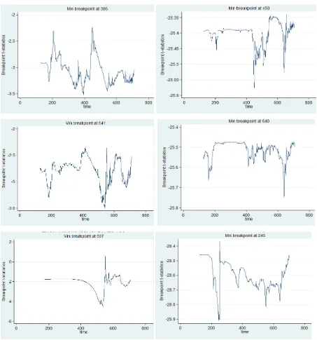
Zivot-Andrews test

The figure 4 illustrates dynamics of t-statistic for all cases. The first column

has statistics for the prices while the second one has for the returns. Each line

corresponds to the returns of the RIN D4, the RIN D5 and the RIN D6,

respectively. The returns are calculated as the difference between the logarithm of

current price and the logarithm of price in the previous time moment.

Figure 4. T-statistics for Zivot-Andrews test.

The dynamics of t-statistic helps to find the minimum and compare with the

25

are the same for all cases, in other words, at the 1% level it is 5.57, at the 5% it is

-5.08 and at the 10% level it is -4.82.

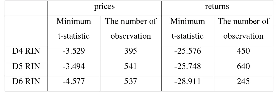
Table 2. Results of Zivot-Andrews test for RIN prices and RIN returns.

prices returns

Minimum

t-statistic

The number of

observation

Minimum

t-statistic

The number of

observation

D4 RIN -3.529 395 -25.576 450

D5 RIN -3.494 541 -25.748 640

D6 RIN -4.577 537 -28.911 245

As it was said in Section 2, the hypothesis about the lack of the unit root is

rejected if value of t-statistic is higher than the critical value absolutely. So

minimum t-statistics for price processes are not high enough to reject the

hypothesis whereas values for the returns case are high significantly. Therefore,

processes of RIN returns are stationary and all models will estimate parameters for

them.

Ljung-Box and ARCH tests

As it was described in Section 2, the null hypothesis, that a process does not

have ARCH effect, is rejected if test statistic is higher than the critical value. Both

tests showed that all series have ARCH effect (Appendix 1), so the type of the

model which should be estimated is MS ARMA-GARCH-M.

3.3. Returns description

For all three series Zivot-Andrews test does not reject the hypothesis that

price process has at least one unit root whereas the test rejects the same hypothesis

for the return process. So we estimate all models using RIN returns.

All returns change in the gap [-0.5; 0.5] except several points of D6 RIN

26

as 3rd and 4th February 2014. These outliers are excluded from the analyzed

sample.

Figure 5. RIN returns

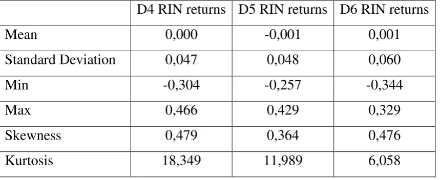
We observe almost zero mean and small standard deviation for all return series (Table 3, where the D6 RIN sample does not have outliers). Minimum points are much the same, but maximum points differ from each other dramatically. Additionally, each series has positive skewness and a usual excess kurtosis for this type of data and sample size.

Table 3. Descriptive Statistics of RIN returns

D4 RIN returns D5 RIN returns D6 RIN returns

Mean 0,000 -0,001 0,001

Standard Deviation 0,047 0,048 0,060

Min -0,304 -0,257 -0,344

Max 0,466 0,429 0,329

Skewness 0,479 0,364 0,476

Kurtosis 18,349 11,989 6,058

3.4. Results of estimation

First of all, we estimate MS GARCH with normal distribution. All results

are presented in Table 4. Regardless of chosen RIN return sample, residuals do not

have standard normal distribution, according to Kolmogorov-Smirnov test. This

-0,4 -0,2 0 0,2 0,4 0,6 03.01.20 11 03.06.20 11 01.11.20 11 03.04.20 12 31.08.20 12 01.02.20 13 03 .07 .20 13 02.12.20 13

D4 RIN returns

-0,4 -0,2 0 0,2 0,4 0,6 03.01.20 11 03 .06 .20 11 01.11.20 11 03.04.20 12 31.08.20 12 01.02.20 13 03.07.20 13 02.12.20 13

D5 RIN returns

-1 -0,5 0 0,5 1 1,5 2 03.01.20 11 03.06.20 11 01.11.20 11 03.04.20 12 31.08.20 12 01.02.20 13 03.07.20 13 02.12.20 13

27

test definitely rejects the hypothesis that the distribution is standard normal,

because probability is too small, it approximately equals 0. Also we can calculate

that the residuals probable have distribution with high parameter than 0 and 1.

Since the definition of GARCH model with normal distribution presupposes

that it has to be standard normal one, so we reestimate model adding additional

restrictions for parameters of distribution. Thus, the model is estimated a way that

residuals have to have zero mean and unit standard deviation. The new values of

parameters are represented in the last three columns of Table 4.

Also we estimate MS GARCH model with two Student-t distributions. If we

ignore the fact that financial assets usually has leptokurtic distribution and estimate

the model using standard normal distribution, then estimators will be consistent

and asymptotically normal, but not efficient.

For the D4 RIN returns changing model from normal distribution to standard

normal one does not influence significantly the parameters, it is a little change of

parameter which reflects the dependence between returns and volatility in a return

equation and conditional probabilities. Moreover, this revision does not impact the

value of likelihood, probably it is because of small lack between -0.0042 and 0 as

well as 1.0303 and 1, in spite of the rejection by Kolmogorov-Smirnov test.

Besides that, for the D4 RIN return choosing of a distribution effect results

and values of parameters dramatically. Also the model with Student-t distribution

has two regimes with similar degree of freedom whereas the model with standard

normal distribution has only one regime, in other words, it is usual

AR(1)-GARCH-M(1,1) model.

In the D5 RIN returns case, making exact standard normal distribution effect

seriously. It does not influence parameters of the second regime, but impact

parameters of the first one, for instance, two parameters become zeros. In addition,

the value of likelihood decreased twofold. Despite of appearance both regimes, the

28

Table 4. Values of estimated parameters

parameter Student-t distribution Normal distribution Standard normal

distribution D4 RIN D5 RIN D6 RIN D4 RIN D5 RIN

D6 RIN D4

RIN

D5

RIN

D6

RIN

-0.475 3.7262 0.0001 0.0005 0.0003 0.0059 0.0005

-0.0006

0.0059

-0.573 0.0003 -0.001 0.0005 0.0003 0.0059 0.0005 0.003 0.0059

0.1570 0.1275 0.2896 0.2292 0.2914 0.2154 0.2292 0.119 0.2154

0.1571 0.2563 0.2785 0.2292 0.2914 0.2154 0.2292 0.2914 0.2154

2.0784 -1.995 -0.142 0.1967 -1.81 -0.345 0.1971 0.7519 -0.345

2.9597 -0.299 -0.062 0.1969 -1.81 -0.345 0.1967 -1.81 -0.345

0.0031 0.9509 0.0021 0.0001 0.0001 0.0072 0.0001 0.0001 0.0072

0.0025 0.0002 0.001 0.0001 0.0001 0.0072 0.0001 0.0001 0.0072

0.0004 0.005 0.9977 0.2732 0.2164 0.305 0.2732 0 0.3050

0.0003 0.5263 0.7182 0.2732 0.2164 0.305 0.2732 0.2164 0.3050

0.9865 0.4911 0 0.7092 0.7618 0 0.7092 0 0

0.987 0.4463 0.2645 0.7092 0.7618 0 0.7092 0.7618 0

0.5678 0.4998 0.5 0.5185 0.1887 0.5047 0.5260 0.5 0.3070

0.5684 0.4999 0.5 0.5185 0.1887 0.5047 0.5260 0.4965 0.3070

mean -0.042 0.0058 -0.0101 0 0 0

std4 1.0303 1.0183 1.0030 1 1 1

5 ₂ 2 2.599

2 3.028 2.796

EL 0.0042 0.0051 0.0051 0.0035 0.0128 0.0039

likelihood 2217.2 2064 1599.6 2049.9 1849.1 486.9 2049.9 1051.1 486.9

4

Standard deviation

5

29

The model with Student-t distribution for the D5 RIN returns also has both

regimes and, in contrast to results of estimation of the model for the D4 RIN

returns, parameters of regimes differ from each other sufficiently. In this case we

receive two distributions with different degrees of freedom.

For the D6 RIN returns the change of normal distribution to standard normal

one impacts only conditional probability, all other parameters are the same. In spite

of the very little difference between parameters of normal distribution with 0 and

1, Kolmogorov-Smirnov test rejects the hypothesis that it is standard normal

distribution again.

In the previous cases with Student-t distribution conditional probability is

approximately 0.5, but for the D6 RIN return it is exactly 0.5. Moreover, changing

distribution significantly has affect on the value of the likelihood, it is less

threefold.

3.5. Results of forecast

Using White’s test, which was described above, we choose the MS GARCH

model with standard normal distribution for all cases as a “better” model, because

value of EL is less than for Student-t distribution (Table 4). Moreover, MS

AR(1)-GARCH-M(1,1) does not forecast zero returns, so we cannot say that this model is

“better” than AR(1)-GARCH(1,1) with excluding zero returns in advance.

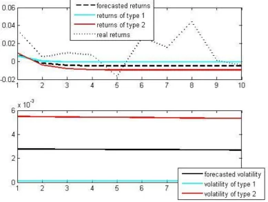
The Figure 6 represents return and volatility forecast for D5 RIN return, it is

the case when we have both regimes. The forecasted returns do not fluctuate the

way which the real data changes, probably it happens because the forecast of

volatility is stable after the fourth step.

Additionally, because of probability which is close to 0.5, the forecasted

volatility is similar as average between high and low volitilities which equals

30

Moreover, it is seen that that the first four steps are forecasted almost right,

because the forecasted returns are not so far from the real returns. It means that

maybe it is better to reestimate model every four or five days and do new forecast.

Figure 6. The forecast of returns and volatility for the D5 RIN

3.6. Comparing the price forecast with the forecast doing by EPA

Except prices of RINs, every day EPA reports its forecast for this day. It

includes bid and ask prices. Bid price is the price at which a participant is prepared

to buy commodity and ask price is the price at which a participant is prepared to

sell commodity. [1.22]

Using received forecast and data which are reported by EPA, we forecast

prices and analyze what forecast is “better”. As it was mentioned in Section 2,

31

Our forecast is not the best way to predict future prices, for example, the D6

RIN prices (Figure 7). Starting the second period our forecast differ dramatically

from the real price whereas the bid and ask prices increase the similar rates. It

means that we do not include a significant factor in our estimation which can

influence the rise of RIN price in this case. Blazsek and Downarowicz [1.3] in their

paper put an additional factor in the return equation. This factor has high

correlation with their data. So probably significant factors enable to forecast RIN

volatility and RIN prices better.

32

Conclusion

The RIN market is a young market, it has big potential for development as

environmentally friendly structure as well as financial one. For nine years of

existence this market has change significantly, for example, EPA which is

regulator of this market understands that it is possible to influence RIN prices

changing level of mandates.

The main actors of financial side of this market are refiners who produce

ethanol and received RINs from EPA for each gallon of ethanol as well as blenders

who buy this ethanol with RINs. Each blender decides how much ethanol is mixed

with gasoline, because there are several types of combination, for example, E10

(10% ethanol and 90% gasoline, E15, E85 and etc.). A blender do not have to buy

all necessary RINs from refiners, it is possible to buy from another blender who

has excess of this financial asset. At the report period blenders should have the

concrete number of RINs which was reported them by EPA. Only 20% of RIN

excess can be kept for the next year, others become invalid.

In this paper we define what RIN means, describe the market structure and

all its actors including refiners, blenders and EPA. Also it has short part about the

last tendency on the market and what is researched now. Besides that, we specify

possible ways to estimate dynamics of a financial asset and forecast returns and

volatility as well as some necessary tests such as Zivot-Andrews, ARCH and

Ljung-Box tests.

According to the main target of this paper to identify MS GARCH model

cannot forecast better than GARCH model, because it cannot forecast zero returns.

Additionally, according to White’s test we identify than standard normal

distribution is better.

At the same time our forecast of volatility using MS GARCH with standard

normal distribution does not work the right way. In other words, forecasted

volatility and returns are not fluctuated and also forecasted returns differ

33

Futhermore, we compare our price forecast with data which are presented by

EPA. Every day it reports bid and ask prices. Using White test again, we measure

the difference between our forecasted prices and real ones as well as the difference

between the average of bid and ask prices and real prices too. The value of

calculated parameter is less in our case. In addition, the price does not change the

way it should do, in other words, maybe we do not include a significant factor in

34

Bibliography

1. Papers:

1.1. Abramson, A., Cohen I.. On the stationarity of Markov switching

GARCH processes // EconometricTheory (2007), vol. 23, pp.

485-500.

1.2. Babcock B., Pouliot S. The Economic Role of RIN Prices. Retrieved

at April 20, 2014, from

http://www.card.iastate.edu/policy_briefs/display.aspx?id=1212

1.3. Bauwens L., Preminger A., Rombouts J., Theory and ingerence for a

Markov switching GARCH model // Econometrics Journal (2010),

vol. 13, pp. 218-244.

1.4. Blazsek S., Downarowicz A., Forecasting hedge fund volatility: a

Markov regime-switching approach // The European Journal of

Finance (2013), vol. 19, no. 4, pp. 243-275.

1.5. Bollerslev T. Generalized Autoregressive Conditional

Heteroskedasticity // Journal of Econometrics (1986), vol. 31 (3), pp.

307–327.

1.6. Carvalhal A., Mendes B., Evaluating the forecast accuracy of

emerging market stock returns // Emerging Market Finance & Trade,

vol. 44, no.1 (2008), pp. 21-40.

1.7. Choi K., Hammoudeh S., Long memory in oil and refined products

market // The Energy Journal, vol. 30, no. 2 (2009), pp. 97-116.

1.8. Dickey, D. A.; Fuller, W. A. Distribution of the Estimators for

Autoregressive Time Series with a Unit Root // Journal of the

American Statistical Association (1979), vol. 74 (366), pp. 427–431 .

1.9. Engle R. Autoregressive conditional heteroskedasticity with estimates

of the variance of U.K. inflation // Econometrica (1982), vol. 50,

pp.987-1008.

1.10. Fama, E. Mandelbrot and the stable Paretian hypothesis. Journal of

35

1.11. Fama, E. The behavior of stock market prices. Journal of Business

(1965a), vol. 38, 34–105.

1.12. Francq C., Zakoian J. Stationarity of multivariate Markov-switching

ARMA models // Journal of Econometrics (2001), vol. 102, pp.

339-364.

1.13. Hamilton, J. A new approach to the economic analysis of

nonstationary time series and the business cycle // Econometrica

(1989), vol. 57, 357-384.

1.14. Hansen P. An unbiased and powerful test of superior predictive

ability, mimeo (2001), Brown University.

1.15. Henneke, J., Rachev S., Fabozzi F., Nikolov M., MCMC-based

estimation of Markov switching ARMA-GARCH models. // Applied

Economics (2011), vol.43, no. 3, pp. 259-271.

1.16. Hill J., Jennings T., Vanezi E., The emissions trading market: risks

and challenges (Financial Service Authority, 2008). Retrieved at April

10, 2014, from

http://www.fsa.gov.uk/pubs/other/emissions_trading.pdf

1.17. Hove J. RIN management and RIN marketing strategies: prepping for

new EPA RIN quality rules. Retrieved at April 15, 2014, from

http://www.rinalliance.com/2013_Jan_RIN%20Management%20and

%20RIN%20Marketing%20Strategies.pdf

1.18. James, T., Fusaro, P., Energy and Emissions Markets: Collision or

Convergence? 2006.

1.19. Kakorina E. RIN market: price behavior and its forecast // Munich

Personal RePEc Archive (2014). Retrieved at April 5, 2014, from

http://mpra.ub.uni-muenchen.de/53715/1/MPRA_paper_53715.pdf

1.20. Karanasos M., Kim J., Moments of the ARMA-EGARCH model //

Econometrics Journal (2003), vol. 6, pp. 146-166.

1.21. Kim C., Nelson C.. State-Space Models with Regime Switching. The

36

1.22. Leppard S., Energy Risk Management. A non-technical introduction

to energy derivatives. 2005

1.23. Klassen F. Improving GARCH volatility forecasts with

regime-switching GARCH // Empirical Economics (2002), vol. 27, pp.

363-394.

1.24. Kolmogorov, A. Sulla Determinazione Empirica di una Legge di

Duistributione // Giornale dell’ Istituto Ialiano delgli Attuar (1933), vol. 4, pp. 1-11.

1.25. Ljung G., Box G. On a Measure of a Lack of Fit in Time Series

Models". Biometrika (1978), vol. 65 (2), 297–303.

1.26. Marcucci J., Forecasting stock market volatility with

regime-switching GARCH models // Studies in Nonlinear Dynamics &

Econometrics, 2005, vol. 9, issue 4, pp. 1-55.

1.27. Mandelbrot B. The variation of certain speculative prices // The

Journal of Business (1963), vol. 36, pp. 394-419.

1.28. McDonald J., Birth time series models and structural interpretations //

Journal of the American Statistical Association, vol.75, no. 369 (Mar.

1980), pp. 39-41.

1.29. McPhal L., Westcott P., Lutman H. The renewable identification

number system and U.S. biofuel mandates // A report from the

Economic Reseach Service (2011). Retrieved at April 10, 2014, from

http://www.ers.usda.gov/media/138383/bio03.pdf

1.30. Miao R., Hennessy D., Bruce A. Babcock investment in cellulosic

biofuel refineries: do waivable biofuel mandates matter? AAEA

annual meetings poster presentation, Denver, CO, July 25-27, 2010.

1.31. Muler N., Pena D., Yohai V., Robust estimation for ARMA models //

The Annals of Statistics (2009), vol. 37, no. 2, pp. pp.816-840.

1.32. Paolella M., Taschini L. An Econometric Analysis of Emission

Trading Allowances // Journal of Banking and Finance (2008), vol.

37

1.33. Perron, P., The great crash, the oil price shock, and the unit root

hypothesis // Econometrica (1989), vol. 57, pp.1361-1401.

1.34. Phillips, P. C. B.; Perron, P. Testing for a Unit Root in Time Series

Regression // Biometrika (1988), vol. 75 (2), pp. 335–346.

1.35. Sabbaghi O., Sabbighi N., Carbon Financial Instruments, thin trading,

and volatility: evidence from the Chicago Climate Exchange // The

Quartely Review of Economics and Finance (2011), vol. 51, pp.

399-407.

1.36. Smirnov N., On the estimation of the discrepancy between empirical

curves of distribution for two independent samples // Bull. Math.

Univ. Moskow (1939b), vol. 2, pp. 3-14.

1.37. Stavins R. Experience with market-based environmental policy

instruments // Discussin paper 01-58, 2008. Retrieved at April 8,

2014, from http://www.rff.org/documents/RFF-DP-01-58.pdf

1.38. Tse Y., Tsui A. A multivariate GARCH model with time-varying

correlations // Journal of Business and Economic Statistics (2002),

vol. 20, no 3, pp. 351-362.

1.39. Whittle P., (1951) Hypothesis Testing in Time Series Analysis.

Thesis, Uppsala University, Almqvist and Wiksell, Uppsala.

1.40. Zivot E., Andrews W. Further evidence on the Great Crash, the

oil-price stock, and the unit-root hypothesis // Journal of Business and

Economics Statistics (1992), vol. 10, no 3, pp. 251-270.

1.41. White H., A reality check for data snooping // Econometrica (2000),

vol. 68(5), pp. 1097-1126.

2. The Internet recourses:

2.1. Analysis of Whether Higher Prices of Renewable Fuel Standard RINs

Affected Gasoline Prices in 2013 // A Whitepaper prepared for the

38

from

http://www.ascension-publishing.com/BIZ/Ethanol-RIN-correlation.pdf

2.2. Countries acting now. Retrieved at April 12, 2014, from

http://www.climatechange.gov.au/international/actions/countries-acting-now

2.3. Court declines to hear challenge to EPA's stance on E15 gasoline. The

Detroit News. Retrieved at February 27, 2014, from.

http://www.biblicalwritings.com/encyclopedia-of-bible-and-theology/?word=Ethanol_fuel_in_the_United_States

2.4. Department of Energy. Retrieved at April 12, 2014, from

http://energy.gov/

2.5. EPA's Themes - Meeting the Challenge Ahead. Retrieved at April 20,

2014, from

http://www2.epa.gov/aboutepa/epas-themes-meeting-challenge-ahead

2.6. Ethanol RINs Market Explodes. Retrieved at March 15, from

http://www.ethanolproducer.com/articles/9753/ethanol-rins-market-explodes

2.7. Historic U.S. fuel Ethanol Production. Retrieved at April 5, 2014,

from http://www.ethanolrfa.org/pages/statistics

2.8. New University Analysis: No Changes Needed to 2014 and 2015

Renewable Fuel Requirements. Retrieved at March 30, 2014, from

http://www.ethanolrfa.org/news/entry/new-university-analysis-no-changes-needed-to-2014-15-renewable-fuel-require/

2.9. RIN fraud not an issue: RINAlliance and EcoEngineers provide

proven success. Retrieved at April 14, 2014, from

http://www.rinalliance.com/RIN_Fraud_Not_An_Issue_PressRelease

39

Appendix

Appendix 1. Results of ARCH and Ljung-Box tests

RIN m ARCH test Ljung-Box (e) Ljung-Box (e^2)

D4 5 H 1 1 1

p-value 0.0032 0.0041 0.0010

ARCHstat/Qstat 17.7774 17.2176 20.5222

Critical Value 11.0705 11.0705 11.0705

10 H 1 1 1

p-value 0.0000 0.0049 0.0000

ARCHstat/Qstat 40.2538 25.2620 53.5790

Critical Value 18.3070 18.3070 18.3070

15 H 1 1 1

p-value 0.0000 0.0000 0.0000

ARCHstat/Qstat 52.8802 51.0660 79.4077

Critical Value 24.9958 24.9958 24.9958

D5 5 H 1 1 1

p-value 0.0813 0.0012 0.0449

ARCHstat/Qstat 11.7937 20.1625 11.3460

Critical Value 11.0705 11.0705 11.0705

10 H 1 1 1

p-value 0.0000 0.0012 0.0000

ARCHstat/Qstat 48.7915 29.0264 57.1199

Critical Value 18.3070 18.3070 18.3070

15 H 1 1 1

p-value 0.0000 0.0017 0.0000

ARCHstat/Qstat 54.2107 36.0569 67.2264

Critical Value 24.9958 24.9958 24.9958

40

p-value 0.0032 0.0041 0.0010

ARCHstat/Qstat 17.7774 17.2176 20.5222

Critical Value 11.0705 11.0705 11.0705

10 H 1 1 1

p-value 0.0000 0.0049 0.0000

ARCHstat/Qstat 40.2538 25.2620 53.5790

Critical Value 18.3070 18.3070 18.3070

15 H 1 1 1

p-value 0.0000 0.0000 0.0000

ARCHstat/Qstat 52.8802 51.0660 79.4077