The Rough Method for Spatial Data Subzone Similarity Measurement

The Rough Method for Spatial Data Subzone Similarity

Measurement

Weihua Liao

School of Mathematics and Information, Guangxi University, Nanning, China Email: [email protected]

Received September 7,2011; revised November 2, 2011; accepted November 28, 2011

ABSTRACT

There are two methods for GIS similarity measurement problem, one is cross-coefficient for GIS attribute similarity measurement, and the other is spatial autocorrelation that is based on spatial location. These methods can not calculate subzone similarity problem based on universal background. The rough measurement based on membership function solved this problem well. In this paper, we used rough sets to measure the similarity of GIS subzone discrete data, and used neighborhood rough sets to calculate continuous data’s upper and lower approximation. We used neighborhood particle to calculate membership function of continuous attribute, then to solve continuous attribute’s subzone similarity measurement problem.

Keywords: Subzone; Rough Sets; Neighborhood Rough Sets; Similarity Measurement

1. Introduction

GIS entity has some spatial relevance in real world. To- ber [1] proposed the famous geography first law “The spatial entities are always interrelated, especially, it have more obvious character for closed distance entities”. Cliff [2] put forward spatial autocorrelation concept from this established law, and the concept is the information for a spatial unit having similarity for it’s around units as sum-marized in Wang [3]. And the spatial autocorrelation has been widely used in many fields, such as regional e- conomy, application ecology, scene analysis, preventive medicine and so on [4]. Anselin [5] found the spatial auto- correlation has two measurement index, that is global in-dex and local inin-dex. Global inin-dex study the spatial mo- de for whole region, and it use a single value to reflect the region’s spatial autocorrelation degree. Local index ca- lculate each unit degree of correlation from its neighbor unit for one attribute. And it has widely application do- main as a similarity problem tool.

GIS subzone measurement is actually an uncertainty study problem. Li [6] found the uncertainty problem stu- dy works have attracted more and more attention by ma- ny study workers since entering the 21st century. There are many mathematic tools for study uncertainty problem, such as fuzzy sets, rough sets, quotient space etc. Rough sets have been widely used in GIS uncertainty study, Pawlak [7] introduced Rough sets theory and discussed in greater detail in Refs [8,9]. It is a technique for dealing with uncertainty and for identifying cause—effect rela-

uni-verse, and took neighbor as basic information particle, then Lin [23] took it to describe others concepts in ap- proximation space. The math pathfinders have done ma- ny study works about rough sets similarity. Wu [24] gi- ven three forms of the differences of rough fuzzy set, and discussed their basic properties, they think that the num- ber of conditions for the difference degree of rough fuzzy set should have must be satisfied. Guan [25] defined the concept of rough similarity degree between two rough sets by using fuzzy sets induced by rough sets, and dis- cussed its properties, and compared four kinds of rough similarity degree in the approximation space.

So it has many studies about similarity measurement for discrete value and continuous value in mathematics. There are two Similarity measurement correlations met- hods in GIS, one is cross-coefficient, and the other is spa- tial autocorrelation that based on spatial location. These two methods can not measure similarity of GIS subzone. This paper use rough sets measurement method to mea- sure two subzone’s similarity problem, simultaneously study the subzone’s similarity based on one universe set.

2. Spatial Autocorrelation and

Cross-Coefficient

2.1. Global Spatial Autocorrelation

Global spatial autocorrelation is an attribute value descri- ption of whole region spatial character. And it estimated global spatial autocorrelation statistic for global Moran’s

I and global Geary’s C, to analyze total region spatial correlation and spatial discrepancy. And global Moran’s

I is used commonly, it is defined as follows:











1

2 0

n n

ij i j

i j n

i i

x x x x

n I

s _{x x}





 

 







(1)

where xi is the observed value for observed spatial cell,

x is the average value for each observed value, S0 is the

sum of all element spatial weight matrix (W), and it can obtained from the follows formula:

0 1 1

n n ij i j

S 

 





(2)

ij

 is the spatial weighting matrix, and the value of ij

can obtain from follows formula:

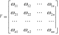
11 12 1

21 22 2

1 2

n n

n n nn

W

  

  

  

 

 

 



 

 

 

     



(3)

where n is the number for spatial cell. And if the i cell and the j cell are neighborhood, then ij= 1, otherwise

ij

 = 0. And one cell is neighborhood for itself, namely

ij

 = 1. It can use Z test to statistic test its result after computing Moran’s I, it can obtain from follows formula (4):

 

 

 

I E I Z I

VAR I 

 (4)

It is frequently took Moran’s I as cross-coefficient, and the value of Moran’s I is between –1 and 1. In given level of significance, when Moran’s I is obviously posi- tive, it indicates each observed value has positive correla- tion, and higher observed value is cluster to higher obser- ved value, lower observed value is cluster to lower obser- ved value, it presents higher to higher cluster or lower to lower cluster. when Moran’s I is obviously negative, it indicates each observed value has negative correlation, and higher observed value is cluster to lower observed value, it presents dispersed pattern. When the Moran’s I

trends to 0, it express that it has no spatial autocorrelation, it is random patterns for spatial observed value.

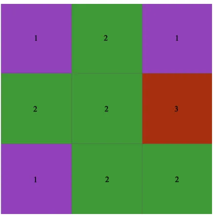
Example 1 considering the example seen in Figure 1,

there are nine polygons, the number ID from left to right, top to down is {1, 2, 3,9}. The label of each polygon in Figure 1 is the value of each polygon. We can see the

value of each polygon is continuous spatial value. Then we can calculate the global Moran’s I value is 0.028508, Z value is 0.636673. So the distribution of Figure 1 is a

dispersed and random spatial pattern.

2.2. Local Spatial Autocorrelation

[image:2.595.120.243.476.524.2]

Global Moran’s I is an overall statistic index, and it only illustrated the average degree of region and adjacent re- gion. Local spatial disparities may expand, when the

[image:2.595.318.524.503.705.2] [image:2.595.123.226.649.710.2]

whole region express a region’s spatial disparities trend we need to use ESDA local analysis method. Anselin (1994) proposed the local spatial relation index LISA (Local Indicators of Spatial Association), it can show the spatial autocorrelation characteristic for local and each spatial cell. It apportioned global Moran’s I to each re- gion, and the i statistic for each region is:

i ij i j

I 



 z z (5) where zi, zj is standardization average value, ij is spa-

tial weighting matrix.

In given significance level, if Ii is obviously positive

and ziis greater than 0, and it indicates that the observed

value of position I and neighborhood are relatively hig- her, it is higher to higher cluster, if it is obviously posi- tive and zi is less than 0, and it indicated that the ob-

served value of position I and neighborhood are rela- tively lower, it is lower to lower cluster, if it is obviously negative and zi is greater than 0, and it indicates that the

neighborhood value is far lower to position I, it is higher to lower cluster, if it is obviously negative and ziis less

than 0, and it indicates that the neighborhood value is far higher to position i, it is lower to higher cluster.

It is weighted average product for observed value of position i and neighborhood. So global Moran’s I and local Moran’s Ii have follows relation:

1 n

i ij j i j i

I z z

n 

 

 _

 

 



j

(6)

The formal condition of LISA statistic and local Mo- ran’s Ii is:

 

,

n i i i

j j i j

I d Z d Z







(7)

We can use Moran scatter plot to describe LISA. All observed value is cross shaft, and all spatial lag value (Wx)

is on ordinate axis. All spatial lag value for each region’s observed value is the weighted average value of neigh- borhood’s observed value. It concretely defined by stan- dardized spatial weighting matrix. The Moran scatter plot can be divided into four quadrants, it is respectively cor- responding to four spatial different region spatial type. The right upper quadrant (HH) is the level for region and its neighborhood are higher, and the spatial disparities degree of both is on the small side. The left upper quad- rant (HL) is the region’s level is lower than its neighbor- hood, and the spatial disparities degree of both are com- paratively large. The left lower quadrant (LL) is the spa- tial level for region and its neighborhood are higher, and the spatial disparities degree of both is on the small side. The right lower quadrant (LH) is the region’s spatial level is higher than its neighborhood, and the spatial dis- parities degree of both is comparatively large.

Example 2 we can compute local Moran’s I of Figure

2, then we can obtain local autocorrelation map, that can

be seen in Figure2. 1) is low and high cluster, 2) is high

and high cluster, 3 is high and low cluster in Figure2.

We can obviously obtain some properties of spatial au- tocorrelation as below:

1) Patial autocorrelation can only compute continuous attribute value, and can not compute discrete categorical data.

2) Spatial autocorrelation can only compute similarity problem of the whole or each unit’s element, and it can not compute for the similarity between subzones that are composed of several units in whole region.

2.3. Cross-Coefficient

The cross-coefficient r is frequently used to measure li- near correlation dimension of two variables in statistics, when xi is not all zero and yi is not all zero, the formula

of cross-coefficient can obtain from follows formula (8):









 

2



2

1 1

i i

n n

i i

i i

x x y y r

x x y y

 

 



 







(8)

where r is the cross-coefficient of variables y and x. x

and y are respectively to the average value of order xi

and i. We can obviously obtain some properties of

cross-coefficient as below:

y

1) Cross-coefficient can only compute continuous at- tribute value, and can not compute discrete categorical data.

2) The length order of xi and must be the same, if

not, it can not compute it. i

[image:3.595.314.533.488.709.2]

y

3. Introduction of Rough Sets Theory

3.1. Concept of Rough Sets

Rough sets theory is a mathematical tool for dealing with uncertainty and vague knowledge. And it is a good tech- nique for dealing with uncertainty and fuzzy of GIS data, it is also a good technique for spatial entity relations. There are many references for studying uncertainty and fuzzy of spatial entity, such as Zhang [26,27].

Definition 1. Given knowledge base K = (U, R), for ea- ch subset XU and an equivalence relation R ind k

 

, we can define two subsets as follows:









RX Y U R Y X

RX Y U R Y X 

   

     (9)

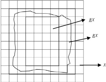
where, RX , RX are respectively called lower appro- ximation and upper approximation of set X. This defini- tion is Pawlak rough sets. If set R is subset of universe, then definable set R is R precise set. If R is a not defin-able set, then R is a rough set. If it has a polygon object X

seen in Figure 3, if we used Pawlak describe it, the

poly-gon object X is a fuzzy object in Figure 3. RX is

defi-nitely belongs to X, RX is possibly belongs to X. Example 3. The classification map of Moran’s I can divide into {{1, 3, 7}{2, 4, 5, 8, 9}{6}} according to e- quivalence class in fig 2. Now it has a subzone X cover- ing {2, 3, 4, 6}, then we can obtain the lower approxima- tion of subzone X is {6}, upper approximation is universe

U. All element’s value must be discrete value when we use Pawlak rough sets partition and compute, but GIS ob- ject attribute’s value is continuous value in practice, such as slope, population density and so on. Then we should use neighborhood rough sets to compute continuous at- tribute value.

3.2. GIS Spatial Data Distance Measurement

Geng (2009) suggested We should measure different att- ribute’s distance in spatial cluster. dijis the distance of

attribute level Xiand Xj. The frequently used distance fo-

rmulas are Minkowski distance, Mahalanobis distance, Canberra distance [28]. We used Mahalanobis distance to define distance of two examples:

 

1

1

q

p _q

ij ia ja a

d q x x

  _ 









 (10)

when q = 1，that is Absolute distance:

 

1

1 p

ij ia ja a

d x







x (11) when q = 2，that is Euclidean distance:

 





2 1 2

1

2 p

ij ia ja a

d x x

 

_ 







when q ，that is Chebyshev distance:

 

1max

ij _{a p} ia ja

d x

 

  x (13) Then, we can obviously see diamond is absolute dis-tance, roundness is Euclidean disdis-tance, square is Cheb- yshev distance in Figure 4.

Example 4. Now we consider it has a GIS map level that composed of nine basic units in Figure 5, B and C

stand for different attribute. Then it should use absolute distance for measure distance x1 and x2 in attribute B, that

we can compute d(x1, x2) = 0.2. It should use Euclidean

distance for measure distance x1 and x2 in attribute B, C,

that we can compute d(x1, x2) = 0.45. We should dispose

source data first in practice, for lack of space, the details will not be dealt with here.

RX RX

[image:4.595.329.512.259.724.2]

X

Figure 3. Rough description of area object.

Figure 4. Neighborhood granules in 2-D spaces.



 (12)

[image:4.595.334.510.282.419.2]

3.3. GIS Continuous Data Granulation and Neighborhood Rough Sets

Li [28] suggested granulation and approximation is the basic problem in rough sets and granular computing. Hu [15] found that Pawlak rough sets are based on the equi- valence class for discrete value space, and the universe partition from equivalence class can divide into univer- se space. But for real number space, the attribute value is continuous, such DEM value etc. Obviously, discrete nu- merical attributes may cause information loss because the degrees of membership of numerical values to discrete va- lues are not considered. Neighborhood structure and or- der structure are important structure for real number spa- ce, so we should work based on neighborhood structure in this paper.

3.3.1. Neighborhood Granulation

There are two methods to define neighborhood, one is defined by the numbers of neighborhood, such as classic k-nearest neighbor methods, the other is defined by dis-tance from one measurement central point to boundary. We used the second method in our work.

Definition 2. Given a N dimension real number space

Ω, we call d is a measurement of RN_{, it usually satisfy}

follows properties:

1) d(x1, x2) ≥ 0, d(x1, x2) = 0, if and only if x1 = x2，

1, 2

N

x x R

  ；

2) d(x1, x2) = d(x2, x1), 1, 2

N

x x R

  ;

3) d(x1, x3) ≤d(x1, x2) + d(x2, x3), 1, ,2 3

N

x x x R

  .

Then we called (Ω, d) is real number space. And Euc- lidean distance is a common measurement tool for real number space.

Definition 3. Given a non-null limited set U{x1, x2, x3, xn} in real number space, for every object xiin U,

then the δ-neighborhood definition is as follows:  

 

x_i



x x U d x x,



, _i





    (14) where δ > 0, 

 

xi is δ neighborhood information

granulation from xi, it for short called as xi neighborhood

granulation.

From the measurement properties, we can get three properties about neighborhood information granulation:

1) 

 

xi  , because of xi

 

xi ；

2) _xj

 

_xi  _xi 

 

_xi

3)

_{ }

i

x U

 



So Given a measurement space (Ω, d) and a non-null limited set U{x1, x2, x3, xn}, if δ1 ≤ δ2, then we can

get these properties:

1)  xi U:1

 

xi 2

 

xi

2) N1N2

Obviously, neighborhood relations are a kind of simi-larity relations, which satisfy reflexivity and symmetry

properties. Neighborhood relations draw the objects toge- ther for similarity or indistinguishability in terms of dis- tances and the samples in the same neighborhood granule are close to each other.

Example 5. Nine polygons are seen in Figure 2, U =

{x1, x2, x3,, x9}, and B and C are respectively stand for

two attribute level value (such as slope, aspect etc), when we choose value in one dimension attribute, we can use absolute distance. We use f (x, b) to express the value in attribute B for example x , then we can get f (x1, b) = 1.6， f (x2, b) = 1.8,, f (x9, b) = 2.1. if we assigned the nei-

ghborhood threshold is 0.2, because of |f(x1, b) – f(x2, b)|

= 0.2 ≤ 0.2, then

 

 

2 1 , 1 2

x  x x  x . In this case, we can get

 

x1



x x x x x1, , , ,2 5 6 7



  ,

 

x₂ 



x x x x₁, , ,_{2 7 8}



,

  

x9 x x x x3, , ,4 8 9



  .

when we get value in two dimension attribute, we should use Euclidean distance, we used f (x, b) to express the value for attribute B, C for example x, if the neighbor-hood threshold is 0.3. Then we can compute each poly-gon’s neighborhood in two dimension space,

 

x1



x x x1, ,5 7



  , 

 

x₂ 



x x₂, 3



,

  

x3 x x x x2, , ,3 4 9



  , 

 

x4 



x x x3, ,4 9



,

  

x5 x x1, 5



  , 

   

x₆  x₆ ,

  

x7 x x x x1, , ,5 7 8



  , 

  

x9  x x x3, ,4 9



.

If it has many attributes, we can compute the distance for examples, and computed the neighborhood for examples.

3.3.2. Neighborhood Approximation

Definition 4. Given a set of objects U{x1, x2, x3,,xn}

and a neighborhood relation R, called D = {U, R} is a neighborhood approximation space [29].

Definition 5. Given D = {U, R} and X ⊆ U. For any

X ⊆ U, two subsets of objects, it is called lower and up- per approximations of X in D= {U, R}, that are defined as follows:

 





 





,

,

i i i

i i i

aprX x U x X x U

aprX x U x X x U

 

 _{   }

 

   

 (15)

Obviously, aprX X aprX .The positive region of X



pos X

 



, negative region of X



neg X

 



and boundary region of X in the approximation space are de-fined as follows:

 

 

 

~

pos X aprX

neg X aprX

bn X aprX aprX

 

 _



 _{ }



(16)

two subsets: positive region and boundary region. Posi- tive region is the set of samples which can be classified into one of the decision classes without uncertainty, whi- le boundary region is the set of samples which can not be determinately classified. Intuitively, the samples in boun- dary region are easy to be misclassified. In data acquire- ment and preprocessing, one usually tries to find a fea- ture space in which the classification task has the least boundary region. It is as summarized in Zhang [26].

Example 6. We given two sets X = {x1, x2, x3, x5, x7}

and Y={x2, x4, x6} in Figure 5, one sets stand for a group

continuous value. Then we can get pos (X) ={x1, x2, x5},

pos (Y) ={x6}, accordingly, we can get the negative re-

gion and boundary region for two sets.

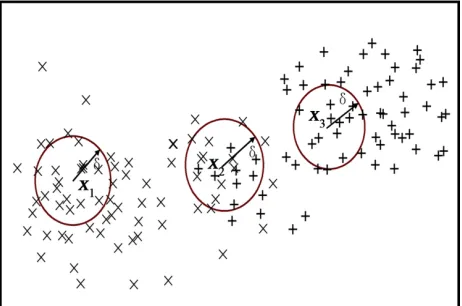
Then we can get a map that shown binary classifica- tion in a 2-D numerical space in Figure 6, it took it as

the first example with “×” label, took it as the second

example with “+” label. So we can see x1 is belongs to

the lower approximations of the first example, x3 is be-

longs to the lower approximations of the second example because of its neighborhood are from the second number,

x2 is boundary example because of its neighborhood is

belongs to the first example and the second example too. The definition is according to our intuitive recognition for classification problem in real world.

4. Rough Measurement Concept

Definition 7. U is universe, R is equivalence relation of U,

A U

  , the rough membership for element x U of set A [30], that are defined as follows:

 

[ ] [ ] R R A R A x x x

   (17) The rough membership of x in A is equal to rough membership for fuzzy set x in equivalence class [ ]xR

that weakly contains to A. So we can understand rough membership as a coefficient, it describe inaccuracy for

x U in A.

The formula (17) is defined for GIS discrete value by Pawlak rough sets membership, but for a continuous va- lue, we can not get equivalence class easily, and we can get this membership from Definition 8.

Definition 8. For GIS continuous value, we use nei- ghborhood rough sets definition for continuous value me- mbership, we defined as follows:

 

_{ }

 

i R A i A x x x    

 (18)

The rough membership of x in A is equal to rough membership for neighborhood information granulation

 

xi

 in equivalence class [ ]xR that weakly contains

to A.

Definition 9. U is universe, R is equivalence relation of

U, A U , then a fuzzy set can get from A and R, via:

 

 

: 0, R A U

x x

R A

  1



, , ,



U u u  u

, ,

(19)

Definition 10. Given universe 1 2 n , R is

equivalence relation of U, A and B are two rough sets of universe U, A B U u iU u, i, the rough membership

about A, B in equivalence relation R is separately

 

R

a_i_A u_i and R

 

i B i

b  u

'_, '

(i = 1, 2,, n), we can get the membership of A and B in equivalence relation R

is separatelyA B

 

, that defined as follows:

 

 

' 1

R R

A A 2

R

A n

 

 

 

1 2

' 1 2

1 2 n R R R B n B B n A

u u u

u

u u

B

u u u

         u    u u     (20)

Then the similarity of set A and B can get from follows formula: [31].













1 1 min , , max , n i i R i n i i i a b SimD A B

else a b         





1, A B   

(21)

We used the formula from Shi [32], it is the similari- ty formula, defined as follows:













1

1

1,

2 min ,

, n i i R i n i i i A B a b SimD A B

else a b              





(22)

Obviously, the higher the similarity of set A and B has, the bigger valueSimD A BR



,



has, vice versa. And it

[image:6.595.309.540.554.707.2]

satisfied these properties:





 

1) SimD A BR ,  0,1





, A B,



;

2) SimD A BR





SimDR ;



,



0

SimD A B 

3) _R ,



1,2,

u U i n

   

if and only if i , one value is at least

0 for R

 

and

A ui

 R

_{ }

B ui

 , and set A and B can not be null at the same time.

5. Case Study

Considering the example seen in Figure 7, it has 100 po-

lygons, the number from left to right, top to down is {1, 2, 3,100}. Now we have three subzone covering poly-gons in Figure 7, that is A, B, C, each subzone covered

16 unit polygons, how to measure these three subzone’s similarity, from membership formula, we can get.

1 2 3 4 5 6 100

0.17 0.17 0.17 0.16 0.17 0.16 0.16

A

x x x x x x x

       

1 2 3 4 5 6 100

0.12 0.12 0.12 0.22 0.12 0.12 0.22

B

x x x x x x x

       

1 2 3 4 5 6 100

0.16 0.16 0.16 0.16 0.16 0.16 0.16

C

x x x x x x x

       





Then the similarity of subzone A and B is:















 







100

1 100

1

2 min ,

,

2 0.12 0.12 0.12 0.16 0.12 0.16

0.8080

0.12 0.17 0.12 0.17 0.16 0.22

i i

i R

i i

i

a b SimD A B

a b



 



    

 

    





 



,



0.9515

SimD A C 



,



0

SimD B CIn a similar way, _R  . So the similarity for R , A and B is less than the similarity of A and C, the similarity for B

and C is less than the similarity of A and C.

.8594

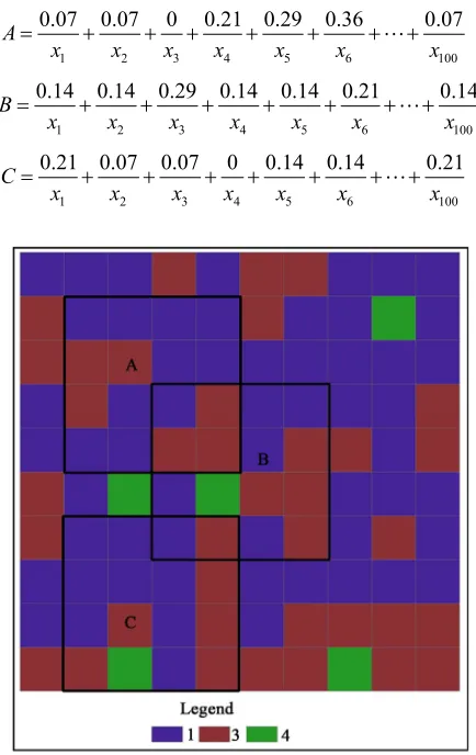
Considering the example seen in Figure 8, it has 100

[image:7.595.314.531.111.455.2]

polygons, the number from left to right, top to down is {1, 2, 3,, 100}. Now we randomly evaluate to every poly- gon’s continuous value (1 - 100), specific value seen in

[image:7.595.59.286.278.488.2]

Figure 8, we have three subzone covering polygons in Figure 8, that is A, B, C, each subzone covered 16 unit

polygons, how to measure these three subzone’s similar-ity for continuous value .

For continuous value in Figure 8, we used absolute di-

stance formula because it only has one attribute, we give threshold δ = 10 for neighborhood granulation. Then we can get each polygon’s distance from others in turns, and get each polygon’s neighborhood information granula-tion. Such as, the neighborhood information granulation of polygon 1 is {1, 10, 27, 28, 34, 50, 51, 65, 68, 75, 94, 98, 99, 100}, the rough membership for subzone A is 1/14, the rough membership for subzone B is 2/14, the

rough membership for subzone C is 2/14. From continu-ous value membership formula, we can get

0.07 0.07 0 0.21 0.29 0.36 0.07

A

1 2 3 4 5 6 100

x x x x x x x

       

1 2 3 4 5 6 100

0.14 0.14 0.29 0.14 0.14 0.21 0.14

B

x x x x x x x

       

1 2 3 4 5 6 100

0.21 0.07 0.07 0 0.14 0.14 0.21

C

x x x x x x x

       

[image:7.595.316.531.480.719.2]

Figure 7. All-around polygon classification and subzone map.

Then the similarity of subzone A and B is:



















 







100

1 100

1

2 min ,

,

2 0.07 0.07 0 0.14 0.14 0.07

0.989

0.07 0.14 0.07 0.14 0.07 0.14

i i i

R

i i i

a b SimD A B

a b









    

 

    





 

In a similar way, SimDR



,C



0.9567, 71

S . So the similarity for A and less than the similarity

the sub si

7. Acknowledgements

nk the project sponsor

REFERENCES

[1] W. R. Tobler Simulating Urban

3

A



,



0.92 R

imD B C 

of A and B, the similarity for B

and C is less than the similarity of A and C. If used spatial autocorrelation to measure

C is

zone milarity for above case, we can find it can not measure

Figure 7, because the value is discrete. And the spatial

autocorrelation can only compute continuous attribute va- lue, it can not compute for the similarity between sub-zones that are composed of several units in whole region. The cross-coefficient can not measure Figure 7 too,

be-cause the value is discrete. And if the subzone in map is not equal length for continuous value, it can not measure similarity too. The rough measurement based on mem-bership function solved this problem well.

6. Conclusion and Future Work

sure similarity This paper used rough membership mea

problem for different subzone. Because Moran’s I can only measure universe or each unit’s spatial autocorrela-tion, it can not measure subzone, so our method can co- mpute GIS subzone similarity based on universe. And for continuous value, we used distance function and nei- ghborhood rough sets to divide continuous value’s upper and lower approximation and classification problem, then we put forward a rough membership function based on neighborhood information granulation. At last, we used rough similarity measurement formula to measure GIS subzone similarity problem, this method can provide a new direction for GIS point group or others’ object group similarity measurement. Our future work should study object group similarity based on different distribution, and for similarity problem based on rough entropy.

The author would like to tha ed by the scientific research foundation of GuangXi University (Grant No.XTZ110584).

, “A Computer Movie

Growth in the Detroit Region,” Economic Geography, Vol. 46, No. 2, 1970, pp. 234-240. doi:10.2307/143141

[2] A. D. Cliff and J. K. Ord, “Spatial Autocorrelation,” Pion,

. Li and Y. Ge, “A Theoretic Framework

pplication of the Integration of London, 1973.

[3] J. F. Wang, L. F

for Spatial Analysis,” Acta Geographica Sinica, Vol. 55 No. 1, 2000, pp. 92-103.

[4] F. Chen and D. S. Du, “A

Spatial Statistical Analysis with GIS to the Analysis of Regional Economy,” Geomatics and Information Science of Wuhan University, Vol. 27, No. 4, 2002, pp. 391-396. [5] L. Anselin, “Local Indicators of Spatial Association:

LI-SA,” Geographical Analysis, Vol. 27, No. 2, 1995, pp. 93-115. doi:10.1111/j.1538-4632.1995.tb00338.x

[6] D. Y. Li and C. Y. Liu, “Artificial Intelligence with

Un-Rough Sets,” International Journal of

Com-wlak, “Rough Sets Theoretical Aspects of

Reason-Theory and Its Application to certainty,” Journal of Software, Vol. 15, No. 11, 2004, pp. 1583-1594.

[7] Z. Pawlak, “

puter and Information Sciences, Vol. 11, 1982, pp. 341- 356.

[8] Z. Pa

ing about Data,” Kluwer Academic Publishers, Dordre- cht, 1991.

[9] Z. Pawlak, “Rough Set

Data Analysis,” Cybernetics and Systems, Vol. 29, No. 9, 1998, pp. 661-668. doi:10.1080/019697298125470 [10] R. Slowinski, “A generalization of the in Discernibility

Relation for Rough Sets Analysis of Quantitative Infor-mation,” Decisions in Economics and Finance, Vol. 15, No. 1, 1992, pp. 65-78. doi:10.1007/BF02086527 [11] P. Srinivasan, “The Importance of Rough

Approxima-tions for Information Retrieval,” International Journal of Man-Machine Studies, Vol. 34, No. 5, 1991, pp. 657-671. doi:10.1016/0020-7373(91)90017-2

[12] T. Beaubouef, F. Petry and B. Buckles, “Extension of the Relational Database and Its Algebra with Rough Sets Techniques,” Computational Intelligence, Vol. 11, No. 2, 1995, pp. 233-245.

doi:10.1111/j.1467-8640.1995.tb00030.x

[13] X. B. Yang, D. J. Yu and J. Y. Yang, “Dominance-Based Rough Set Approach to Incomplete Interval-Valued In-formation System,” Data & Knowledge Engineering, Vol. 68, No. 11, 2009, pp. 1331-1347.

doi:10.1016/j.datak.2009.07.007

[14] T. Beaubouef, F. E. Petry and R. Ladner, “Spatial Data Methods and Vague Regions: A Rough Sets Approach,” Applied Soft Computing, Vol. 7, No. 1, 2007, pp. 425-440. doi:10.1016/j.asoc.2004.11.003

[15] Q. H. Hu, D. R. Yu and Z. X. Xie, “Numerical Attribute Reduction Based on Neighborhood Granulation and Rough Approximation,” Journal of Software, Vol. 19, No. 3, 2008, pp. 640-649. doi:10.3724/SP.J.1001.2008.00640 [16] H. Xie, H. Z. Cheng and D. X. Niu, “Discretization of

Continuous Attributes in Rough Sets Theory Based on Information Entropy,” Chinese Journal of Computers, Vol. 28, No. 9, 2005, pp. 1570-1574.

Engineering, Vol. 16, No. 12, 2004, pp. 1457-1471. doi:10.1109/TKDE.2004.96

[18] D. Dubois and H. Prade, “Rough Fuzzy Sets and Fuzzy Rough Sets,” International Journal of General Systems, Vol. 17, No. 2, 1990, pp. 191-209.

doi:10.1080/03081079008935107

[19] Q. H. Hu, D. R. Yu and Z. X. Xie, “Fuzzy Probabilistic Approximation Spaces and Their Information Measures,” IEEE Transactions on Fuzzy Systems, Vol. 14, No. 2, 2006, pp. 191-201. doi:10.1109/TFUZZ.2005.864086 [20] D. S. Yeung, D. G. Chen, et al., “On the Generalization

of Fuzzy Rough Sets,” IEEE Transactions on Fuzzy Sys-tems, Vol. 13, No. 3, 2005, pp. 343-361.

doi:10.1109/TFUZZ.2004.841734

[21] Q. H. Hu, D. R. Yu and Z. X. Xie, “Information-Pr- eserving Hybrid Data Reduction Based on Fuzzy Rough Techniques,” Pattern Recognition Letters, Vol. 27, No. 5, 2006, pp. 414-423. doi:10.1016/j.patrec.2005.09.004 [22] R. Slowinski and D. Vanderpooten, “A Generalized

Defi-nition of Rough Approximations Based on Similarity,” IEEE Transactions on Knowledge and Data Engineering, Vol. 12, No. 2, 2000, pp. 331-336.

doi:10.1109/69.842271

[23] T. Y. Lin, “Data Mining and Machine Oriented Modeling: A Granular Computing Approach,” Applied Intelligence, Vol. 13, No. 2, 2000, pp. 113-124.

doi:10.1023/A:1008384328214

[24] R. M. Wu and X. H. Zhang, “A Research on the

Rough

Simi-. Liang, “Rough Set

tering

d Knowledge

Discov-nder Rough

Similarity Direction

Shi, “Measure of

i and Y. P. Lian, “Measure of Similarity between ence Measures of Rough Fuzzy Sets,” Journal of South-west University for Nationalities (Natural Science Edi-tion), Vol. 35, No. 6, 2009, pp. 1139-1142.

[25] Y. Y. Guan and H. K. Wang, “Measures of

larity between Sets,” Fuzzy Systems and Mathematics, Vol. 20, No. 1, 2006, pp. 134-139.

[26] W. X. Zhang, W. Z. Wu and J. Y

Theory and Method,” Science Press, Beijing, 2005. [27] X. P. Geng, X. C. Du and P. Hu, “Spatial Clus

Method Based on Raster Distance Transform for Ex-tended Objects,” Acta Geodaetica et Cartographica Sinica, Vol. 38, No. 2, 2009, pp. 162-168.

[28] X. F. Li and J. Li, “Data Mining an ery,” Higher Education Press, Beijing, 2003. [29] Y. Zhou, H. Lin and Y. B. Cui, “The Study u

Relation and It’s Neighbor Relation,” Computer Science, Vol. 31, No. 10A, 2004, pp. 61-63.

[30] F. C. Liu, “Similarity Measure and

between Fuzzy Rough Sets,” Computer Engineering and Applications, Vol. 35, 2005, pp. 63-66.

[31] H. K. Wang, Y. Y. Guan and K. Q.

Similarity between Rough sets and Its Application,” Com-puter Engineering and Applications, Vol. 31, 2004, pp. 39-40.

[32] Z. H. Sh