Application of EMD as a Robust Adaptive Signal Processing Technique in Radar/Sonar Communications

Application of EMD as a Robust Adaptive

Signal Processing Technique in

Radar/Sonar Communications

CH.KUSMA KUMARI*

Research Scholar,

Department of Electronics& Communication Engineering, Andhra University, Visakhapatnam

[email protected]

PROF. K.RAJA RAJESWARI

Professor,

Department of Electronics& Communication Engineering, Andhra University, Visakhapatnam

[email protected]

Abstract:

This paper presents the usage of Empirical Mode Decomposition (EMD) based Robust Adaptive Signal processing Technique that can be used for the analysis of signal which is combined with noise. The simulation results demonstrate the effectiveness of the presented system in noise reduction without changing the signal characteristics.

Key words: LMS, RLS, EMD, IMF, sifting process, monotonic function, noise reduction.

1. Introduction

One important issue in signal processing is Noise-reduction. Noise is considered as any unwanted signal that interferes with the information signal. The original signal can be a bio-medical signal, a speech signal, a radar signal or any other type of signal which conveys useful information from one place to another. The noise signal which may be a Gaussian or non-Gaussian is getting interfered either at the transmitter or in the channel or at the receiver causes degradation of the original signal. We need proper modeling technique to perform de-noising. Some of the Techniques are:

1.1 Linear filter

The simple method for signal de-noising is to employ some type of linear filter to remove the noise from the signal. The problem with this technique is that the spectrum of the noise must be known for the appropriate filter to be constructed and the signal needs to be stationary, which is usually not the case for real signal. In the real environment the signal may be nonlinear, non-stationary etc for which the use of linear filtering is somewhat a tedious process to eliminate the noise from the original signal.

1.2 Short Time Fourier Transform (STFT)

1.3 Adaptive filters

Adaptive filters are essentially digital filters with self-adjusting characteristics. These are mostly used at conditions (1) where the filter characteristics are to be varied i.e. adapted to changing conditions, (2) where there is spectral overlap between the signal and noise and (3) if the band occupied by the noise is unknown or varies with time. Because of these self adjusting performance and in-built flexibility, adaptive filters are used in the applications like telephone echo cancelling, radar signal processing, navigational system equalization of communication channels and bio-medical signal enhancement.

Adaptive algorithms are used to adjust the coefficients of the digital filter such that the error signal is minimized according to some criterion. Common algorithms that have found widespread application are Least Mean Square (LMS), Recursive Least Squares (RLS) etc. LMS is most efficient in terms of computation and storage requirements. It does not suffer from numerical instability problem inherent in other algorithms. But LMS exhibits poor performance for effect of non-stationary and for the effect of signal component on the interference input channel. Hence clearly we can say that LMS is not suitable for real-time or on-line filtering applications. However RLS algorithm has superior convergence properties. For continuous data processing and to improve the estimates, RLS methods are preferred because the estimates are updated for each set of data acquired without repeatedly solving the time-consuming matrix inversion directly. But RLS also suffers with the blow up problem (occurs when there is no input signal for longer time) and is also very much sensitive to computer round off errors which results in negative values that leads to instability. One solution to avoid these problems is to use some factorization algorithms along with the basic RLS algorithm that increases the complexity. [1]

2. Empirical Mode Decomposition (EMD)

EMD is an emerging method in Signal Processing proposed by Norden Huang et.al of NASA [2] in 1998. This method is very much suitable for non-linear & non-stationary signal analysis. The EMD algorithm decomposes the signal y1(t) into narrow band oscillatory components called Intrinsic Mode Functions (IMF) ci(t), i=1,2…N and with a final residue signal r(t).



=

+

=

1 i

i

(

t

)

r(t

)

c

y1(t)

where N means the number of IMF functions. Residue r(t) reflects the average trend of a signal y1(t) or a constant value. IMF’s are the signals with the following characteristics: (1) In the whole data set, the number of extremes (maxima & minima) and the number of zero crossings must either equal or must differ by a maximum of one. (2) Each point, that is defined as mean value of envelopes defined by local maxima and local minima is zero. The decomposition method used in the EMD is called as “Sifting” process.

The biggest advantage of this method is that it is totally adaptive and data driven, without the need for a prior basis function selection for signal decomposition. The EMD has been widely used for data analysis such as Image processing, Bio-signals processing [3], Seismic analysis and detecting [4] mechanical faults of rotating machines and many applications.

The algorithm proceeds in the following steps (see in Fig.1) [5]:

(1) Create upper envelope ‘maxenv(t)’ by local maxima and lower envelope ‘minenv(t)’ by local minima of data y1(t).

(2) Calculate the mean of upper envelope

and lower envelop

2

(t)

minenv

(t)

maxenv

(t)

m

1

+

=

(3) Subtract the mean from original data

h

(t)

=

y1(t)

-

m

(t)

(4) Verify that h1(t) satisfies conditions for IMF’s. Repeat steps 1 to 4 with h1(t) until it is an IMF.

(5) Get first IMF (after k iterations)

c

(

t

)

=

h

(

t

)

−

m

(

t

)

r

(

t

)

=

y1(t

)

−

c

(

t

)

(8) After N iterations y1(t) is decomposed according to Eq. (1). By selecting appropriate IMF’S the de-noised signal can be achieved.

3. Simulation Results

Let us consider a random signal

y(t)

=

sin

(t)

+

sin

(2

*

t)

+

sin

(3

*

t)

for t = 0: 1/1000: 10. In order to use the EMD as robust adaptive signal processing technique the signal is combined with some random noise and an input signal y1(t) is applied to the algorithm for de-noising. For comparison the same signal y1(t) is also applied to LMS and RLS adaptive filtering algorithms to de-noise the signal and simulation outputs are presented in the following figures.

Figure.2 describes the de-noising capability of LMS for the order 28, 29. Up to order 28 LMS is exhibiting somewhat better performance, but when the order is greater-than 28 this algorithm is not able to de-noise the signal.

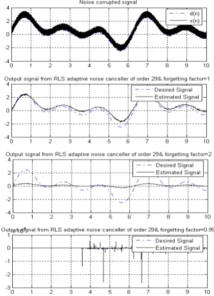
Figure.3 describes the de-noising capability of RLS for the order 29 and for different forgetting factors. Irrespective of the order RLS is exhibiting better performance if the forgetting factor is 1, but if the forgetting factor is varied then this algorithm is not able to de-noise the signal.

Fig: 1. Flow diagram of EMD algorithm. N=1; r (t) = y1 (t)

Obtain all the Extremes of y1 (t)

Calculate Upper envelop ‘maxenv(t)’ and Lower envelop ‘minenv(t)’ by interpolation

Compute the local mean as m(t)=[maxenv(t)+minenv(t)]/2

h(t)=y1(t)-m(t)

IS h(t) an IMF

N=N+1 Cn(t)=h(t) r(t)=r(t)-Cn(t)

Is r(t) a monotonic function

End of EMD

y1(t)=r(t) y1(t)=h(t)

NO

YES

NO

Now the signal is analyzed using EMD algorithm. Figure.4 (a) is the input signal y(t). Figure.4 (b) is the noise added input signal y1(t) that is applied to EMD process. From Figure.4(c) to Figure.4 (n) IMF’s are calculated. Figure.4 (o) is the de-noised signal which is similar as the input signal In this particular EMD process to obtain the de-noised output the first six IMF’s (i.e. from Figure. 4 (c) to Figure. 4 (h)) are not considered, only the remaining six IMF’s (i.e. from Figure. 4 (i) to Figure. 4 (n)) are added to obtain the noise suppressed signal at the output. The addition of IMF’s will be depending on the type of signal considered for the analysis.

From the Figure.4 we can observe that the original input signal which is shown in (a) is similar with the output signal shown in (o). Hence by using EMD process as a robust adaptive filtering technique, the noise signal is eliminated in the original signal.

Fig: 4. (a) Input Signal (b) Noise added input signal (c) to (n) IMF’s calculated using EMD process (o) De-noised Output signal

4. Conclusion

Thus Empirical Mode Decomposition is one of the best methods to reduce the noise present in a received signal. EMD does not depend on any parameter and does not require prior estimates as in the case of adaptive filtering techniques [6]. This method can be applicable in radar/sonar communications to achieve high signal to noise ratio. This method can also be used in real environment to analyze non-stationary signals.

EMD is also applicable to obtain various parameters to improve the performance of the Direction of Arrival (DOA) estimation for sound signals in SONAR application which is the future scope of this paper.

Acknowledgements

This work is being supported under the project “Robust Signal Processing Techniques for RADAR/SONAR Communications using VLSI Tools by Ministry of Science & Technology, Department of Science & Technology (DST), New Delhi, India, under Women Scientist Scheme (A) with the Grant No: 100/ (IFD)/8893/2010-11.

References

[1] “Digital Signal Processing” A practical approach by Emmanuel C.Ifeachor, Barrie W.Jerris.

[2] N.E. Huang, Z. Shen, S.R. Long, M.L. Wu, H.H. Shih, Q. Zheng, N.C. Yen, C.C. Tung and H.H. Liu, “The empirical mode decomposition and Hilbert spectrum for nonlinear and non-stationary time series analysis,” Proc. Roy. Soc London A, Vol. 454, pp. 903–995, 1998.

[3] Karagiannis and P. Constantinou “Investigating Performance of Empirical Mode Decomposition Application on Electrocardiogram” 2010 5th Cairo International Biomedical Engineering Conference Cairo, Egypt, December 16-18, 2010.

[4] Jiajun Han and Mirko van der Baan “Empirical Mode Decomposition and Robust Seismic Attribute Analysis” Recovery – 2011 CSPG CSEG CWLS Convention.

[5] P. Trnka and M. Hofreiter “The Empirical Mode Decomposition in Real-Time” 18th International Conference on Process Control June 14– 17, 2011, Tatranská Lomnica, Slovakia