Mechanisms in wing-in-ground effect aerodynamics

(1)

Mechanisms in Wing-In-Ground Effect

Aerodynamics

M arvin A lan Jones

U niversity College London

University of London

A thesis su b m itted for th e degree of

D o c to r o f P h ilo so p h y

(2)

ProQuest Number: U644143

INFORMATION TO ALL USERS

The quality of this reproduction is dependent upon the quality of the copy submitted.

In the unlikely event that the author did not send a complete manuscript and there are missing pages, these will be noted. Also, if material had to be removed,

a note will indicate the deletion.

uest.

ProQuest U644143

Published by ProQuest LLC(2016). Copyright of the Dissertation is held by the Author.

This work is protected against unauthorized copying under Title 17, United States Code. Microform Edition © ProQuest LLC.

ProQuest LLC

789 East Eisenhower Parkway P.O. Box 1346

(3)

To my Parents

for giving me the opportunity to learn and to understand.

To my Teachers

for showing me how to w rite it down.

To my Sister

(4)

Acknowledgements

I would like to th an k Professor Frank Sm ith for his encouragem ent and guidance as

my supervisor, Dr. Sean O ughton and Dr. Sergei T im oshin for all th eir advice and

assistance, and th e Engineering and Physical Sciences Research Council for their

financial support. I would also like to th a n k all th e lads from th e UCL football

team for providing an escape from th e stu d y of ‘how aeroplanes fly’as they liked to

call it. Finally, I would like to th a n k my family and Loraine for th eir support and

(5)

Abstract

An aircraft in low-level flight experiences a large increase in lift and a m arked re

duction in drag, com pared w ith flight a t altitude. This phenom enon is term ed the

‘w ing-in-ground’ effect. In these circum stances a region of high pressure is created

beneath th e aerofoil, and a pressure difference is set up betw een its upper and lower

surfaces. A pressure difference is not p e rm itte d a t th e trailing edge and therefore a

mechanism m ust exist which allows th e pressures above and below to adjust them

selves to produce a continuous pressure field in th e wake. It is th e stu d y of this

mechanism and its role in th e aerodynam ics of low-level flight th a t forms th e basis

of our investigation. We begin in C h ap ter 2 by considering th e flow p ast a th in aero foil moving a t m oderate distances from th e ground, th e typical ground clearance a

being of order unity. T he aforem entioned m echanism is introduced and described in

detail in th e context of this inviscid problem . C h ap ter 3 considers th e sam e flow for

large and small ground clearances and in th e later case shows th a t th e flow solution

beneath th e aerofoil takes on a p articu larly simple form. In th is case th e lift is shown

to increase as a~^. In C hapter 4 we focus on th e flow p ast th e trailing edge of an

aerofoil moving even nearer th e ground, w ith th e ground ju st outside th e boundary

layer. We show th a t in this case our asym ptotic theory for small a is consistent

w ith a ‘triple-deck’ approach to th e problem which incorporates ground effects via

a new pressure-displacem ent law. T he triple-deck ground-interference problem is

stated and solved. In C hapter 5 we investigate th e case where th e aerofoil is so near

th e ground th a t th e ground is inside th e boundary layer. Here th e moving ground

interacts w ith th e aerofoil in a fully viscous way and th e non-linear boundary layer

equations hold along th e entire length of th e aerofoil. Again a pressure difference at

th e trailing edge is not p erm itted and th is produces up stream adjustm ent back to

th e leading edge. Regions of reversed flow can occur and th eir effects, w ith regard to

downforce production and racing car u n d ertray design, are considered. In C hapter

(6)

C ontents

1 In trod u ction 15

2 Inviscid ‘W in g-In -G rou n d ’ E ffect 27

2.1 In tr o d u c tio n ... 27

2.2 Problem F o r m u la tio n ... 29

2.3 M athem atical M e th o d s ... 31

2.3.1 Sym m etry A rgum ents ... 31

2.3.2 T he Solution ...32

2.3.3 Com pleting th e B oundary C o n d itio n s ...34

2.3.4 T he Pressure Difference Solution ... 42

2.4 N um erical M e th o d s ...43

2.4.1 T he E valuation of th e Pressure Difference [p] ( a : ) ... 43

2.4.2 T he Evaluation of -0 (x) 43

2.4.3 T he Evaluation of h { x ) and M { x , ^ )... 45

2.4.4 T he Evaluation of f (x) 46 2.4.5 The Evaluation of (p) (x) and {v) { x ) ...48

2.5 Flow P r o p e r tie s ...52

(7)

C O N T E N T S 5

3 Inviscid S olu tion s for ^ 1 and ^ <K 1 57

3.1 I n tr o d u c tio n ... 57

3.2 Problem F o r m u la tio n ...60

3.3.1 Fourier Transform ing th e Integral E q u a t i o n s ... 60

3.4 Flying High > 1 ) ...62

3.4.1 T he Leading O rder Solution for ^ 1 ...63

3.4.2 T he Next O rder C orrection for Z$> 1 ...65

3.5 Flying Low (/5 1) ...66

3.5.1 T he Leading O rder Solution for <K 1 ...68

3.5.2 T he In-Between O rder Solution for /? <C 1 ...70

3.5.3 T he Next O rder C orrection for ^ 1 ... 71

3.6 Edge F l o w s ... 72

3.6.1 T he Trailing Edge N o n -E ig e n so lu tio n ... 73

3.6.2 The Leading Edge E ig en so lu tio n ... 83

3.6.3 Setting th e C onstants po- (0), P f - (0), and p i_ ( 0 ) ... 85

3.7 T he Global Solution for 1 ...88

3.8 Flow P r o p e r tie s ...89

4 V iscou s-In viscid ‘W in g -In -G ro u n d ’ Effect 91 4.1 I n tr o d u c tio n ... 91

(8)

C O N T E N T S 6

4.3 M athem atical M e th o d s ...97

4.3.1 T he Solution of th e Interaction Law E q u a tio n s ...98

4.3.2 T he E valuation of th e Fam iliar Interaction L a w s ...100

4.3.3 T he Stream function-V orticity F o r m u la tio n ...102

4.4 N um erical M e th o d s ...104

4.4.1 The Basic D is c r e tis a tio n ... 105

4.4.2 The D iscretised W iener-Hopf Solution A l g o r i t h m ... 106

4.4.3 T he D iscretised Interaction L a w s ...109

4.4.4 T he Solution of th e B oundary Layer E quations ... 110

4.5 F urther C o m m e n t s ...116

4.6 Flow P r o p e r t ie s ... 117

5 V iscou s ‘W in g -In -G ro u n d ’ Effect 121 5.1 In tr o d u c tio n ... 121

5.2 Problem F o r m u la tio n ... 123

5.3.1 T he Flow D irectly B eneath th e Aerofoil ... 128

5.4 Num erical M e th o d s ...130

5.4.1 T he Basic D is c r e tis a tio n ... 131

5.4.2 T he Difference E q u a tio n s ... 132

5.4.3 T he Starting Profiles for 'ifj and Q, N ear x = 0 ... 133

(9)

C O N T E N T S 7

5.4.5 Finding th e Pressure P- {x) ... 135

5.5 Flow P r o p e r t i e s ... 136

5.5.1 Wake Effects ...148

6 T unnel E ffects 155 7 C onclusions and Further W ork 161 7.1 Sum m ary ...161

7.2 F urther W o r k ... 163

A T h in Layers and th e Triple D eck S tru ctu re 165 A .l B oundary L a y e r s ... 165

A. 1.1 T he Blasius B oundary L a y e r ... 167

A .1.2 T he G oldstein Near W a k e ... 168

A .2 The Triple D e c k ... 170

A .3 Diffusion L a y e r s ... 174

B W ien er-H o p f C alcu lation s 177 B .l I n tr o d u c tio n ... 177

B.2 C alculating i? (A)_^ and R { K ) _... 178

B.3 C alculating th e C onstant A ...179

B.4 C alculating th e C onstant // 181

(10)

C O N T E N T S 8

C T riple-D eck S tu d y P rob lem s 187

C .l I n tr o d u c tio n ...187

C.2 Flow P ast a Bum p on a F lat P late in Surface E f f e c t ...189

C.2.1 Problem F o rm u la tio n ... 189

C .2 .2 Small Bum ps {h <^1) 191

C.2.3 Larger B u m p s ...193

C.3 Flow P ast th e Trailing Edge of a F lat P la te in Sym m etric Tunnel Effect 196

(11)

List o f Figures

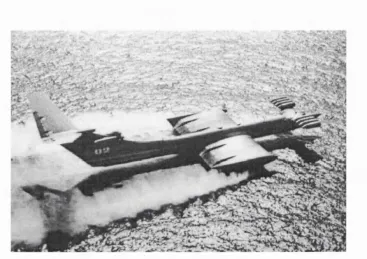
1.1 T he KM Ekranoplan, designed by R otislav Alexiev, w ith its relatively short stubby wings and Y -shaped ta il...18

1.2 The KM E kranoplan as viewed from the side... 18

1.3 The X-112, designed by Alexander Lippisch, w ith its reverse

delta-wing planform ...19

1.4 The X-112 as viewed from th e side...19

1.5 The A m phistar designed by D im itri Sinitsyn. The m odern incarna

tion of th e KM ekranoplan 21

1.6 T he F lairb o at, desined by G unther Jorg, w ith its tan d em aerofoil

configuration...21

1.7 T he Airfisch 3 designed by Hanno Fischer. T he m ost m odern incar

nation of th e Lippisch X-112...22

1.8 T he Hover wing, also designed by H anno Fischer, w ith its unique cata

m aran /hovercraft take-off system ...22

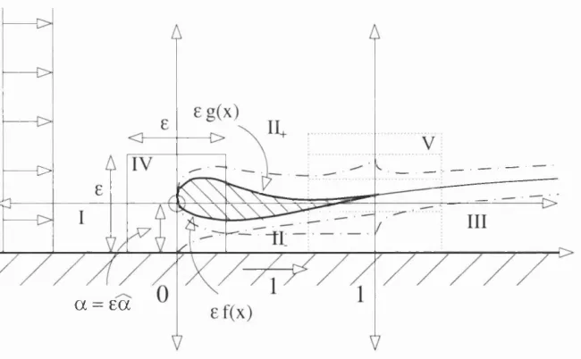
2.1 Cross-section of an aerofoil of thickness e w ith two viscous boundary

layers and a th in viscous wake flying a t a ground clearance a ...33

2.2 Sym m etry argum ents lead to th e introduction of a v irtu al image aero foil beneath th e g r o u n d ... 33

(12)

L I S T OF F IG U R E S 10

2.3 T he integration contours T+, T=, and T_ are defined in th e complex

C plane as above ... 35

2.4 T he pole in the integrand m ust be circum navigated when z is on the surface of th e a e ro fo il...35

2.5 T he functions / (x), h (a;), M (rr, {), a n d '0 (a:) for a = 0.5... 50

2.6 T he sums and differences [p] (a:), (p) (x), [u] (x), and (v) (x) for a = 0.5. 50 2.7 T he pressures and velocities p± (x) and v± (x) for a = 0.5... 50

2.8 The pressure p ertu rb atio n p { x , y ) for a = 0.5... 51

2.9 The transverse velocity p e rtu rb atio n v (x, p) for a — 0.5...51

2.10 The stream w ise velocity p e rtu rb atio n u (x, y) for a; = 0.5...51

2.11 The to ta l displacem ent thicknesses (x) of a horizontal fiat plate aerofoil in ground effect for a = 16 to T ...53

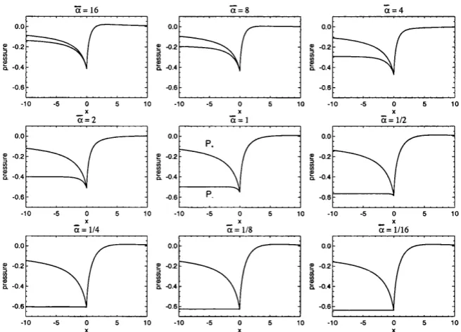
2.12 The pressures p± (x) on a horizontal fiat p late aerofoil in ground effect for a = 16 to T ...53

2.13 T he displacem ents (x) of a fiat p late aerofoil in ground effect at positive angle of a tta ck for o; = 16 to ^ ... 55

2.14 T he pressures p± (x) on a fiat p late aerofoil in ground effect a t positive angle of a tta ck for a = 16 to ^ ... 55

2.15 T he displacem ents ô± (x) of a fiat plate aerofoil in ground effect at negative angle of a tta ck for a = 16 to ^ ... 56

(13)

3.2 T he ‘around-the-edge’ eigensolution which is p erm itted only a t the

leading edge (II) and th e stream lined non-eigensolution which may

occur a t either th e trailing edge (III) or th e leading edge...59

3.3 N um erical solutions for th e pressures (a;) and p_ (x) for a = ^ as

com puted using th e m ethod developed in C h ap ter 2... 90

3.4 A nalytic global solutions for the pressures (x) and p_ (x) ioi a = ^

as calculated using th e small (3 theory developed in this chapter. The

leading edge eigensolution has been added to th e global solution of

section 3.7, however th e non-eigensolutions have n o t... 90

4.1 T he triple deck flow stru ctu re a t th e trailing edge of an aerofoil in

ground effect. Shows th e lower decks (I±), th e m ain decks (II±), th e

upper deck (III), and th e ground diffusion layer (IV) ... 93

4.2 T he interactive ground effect mechanism. Pressure continuity, in the

wake, drives a displacem ent effect which in tu rn drives a pressure

correction and so o n ...93

4.3 T he triple deck pressures P± (V ) for a flat p late in ground effect for

Q = 16 to ^ ... 118

4.4 T he triple deck displacem ent gradients A'^ (X ) for a flat plate in

ground effect for â = 16 to ^ ... 118

4.5 T he triple deck displacem ents A± (X ) for a flat p late in ground effect

for â = 16 to ...119

4.6 T he norm alised skin frictions (X, 0) on th e trailin g edge of a flat

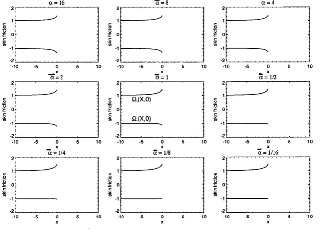
p late in ground effect for â = 16 to ^ ...119

(14)

L I S T O F F IG U R E S 12

5.2 Cross-section of a th in aerofoil in extrem e ground effect. T he bound

ary layers associated w ith th e aerofoil and th e ground merge produc

ing a fully viscous solution beneath th e aerofoil... 124

5.3 The linearly expanding diffuser shape w ith front wheel (not to scale). 137

5.4 The proposed step change in height diffuser shape, which according

to lubrication theory produces more downforce th a n th e linearly ex

panding one... 137

5.5 Several examples of stream wise velocity profiles u ( x , y ) , a t varying

X stations, for forward flow at d = 1, ^ = 1/2, and 7 = 1 /3 ... 138

5.6 Several examples of stream wise velocity profiles u { x , Y ) , a t varying

X stations, for a reversed flow case a t d = 1, /? = 2, and 7 = 1 / 3 .. . . 138 5.7 The stream lines of constant ' ip{x,Y) for d = 16 to /3 = 1, and

7 = 1 directly beneath th e diffuser ...140 5.8 The pressures p± (x) for d = 16 to ^ = 1, and 7 = ^ directly

b eneath the diffuser. Note th e changes of scale betw een each row of

g raphs... 141

5.9 The skin frictions {x) and flo (3;) for d = 16 to ^ , ^ = 1, and

7 = 1 directly beneath th e diffuser ...141 5.10 The stream lines of constant 'ip{x^Y) for d = 1, /3 = 16 to and

7 = 1 directly beneath th e diffuser ... 143 5.11 The pressures p± (æ) for d = 1, ^ = 16 to and 7 = ^ directly

b eneath th e d iffu se r... 144

5.12 The skin frictions [x) and LIq(3:) for d = 1, ^ = 16 to and

7 = 1 directly beneath th e diffuser ... 144 5.13 The stream lines of constant i p ( x ^ Y) for d = 1, P = 1, and 7 = 0 to

(15)

5.14 T he pressures (x) for a = 1, /? = 1, and 7 = 0 to 1 directly beneath th e diffuser ... 147

5.15 T he skin frictions (x) and Ho (a;) for S = 1, jS = 1, and 7 = 0 to 1 directly b en eath th e d if f u s e r ... 147

5.16 The non-dim ensional lift L as a function of th ro a t length 7 and expan sion param eter ^ as calculated as p a rt of m any num erical boundary-

layer s o lu tio n s ... 149

5.17 T he non-dim ensional lift L as a function of th ro a t length 7 and ex pansion param eter /3 as calculated using lubrication t h e o r y ... 149

5.18 Wake results showing stream lines, pressures, and skin frictions for

forward and separated flows. Notice th e reduced pressure variation

in th e right hand case... 151

5.19 Stream lines of constant Tp {x^Y) showing th e extrem ely small closed

eddy close to th e trailing edge... 152

5.20 T he flow topology close to th e trailing edge as observed in the nu

m erical wake solutions (not to scale)...154

5.21 A sim ilar flow topology envisaged for vortex shedding behind a cir

cular cylinder... 154

6.1 Cross-section of a th in aerofoil w ith b oundary layers and a th in vis cous wake moving through a tu n n e l... 158

6.2 T he doubly periodic cascade of image aerofoils introduced due to

sym m etry conditions being applied on the tu n n el floor and ceiling. . . 159

6.3 Integration contours T2n± in th e complex plane corresponding to the

(16)

A .l T he solution to the equation / " ' (77) + ( 77) / " (77) = 0 w ith / (0) = 0, / ' (0) = 0, and / ' ( +00) = 1... 169

A.2 The solution to th e equation g”' (77) + | p (77) (77) — (77)^ = 0 w ith

g (0) = 0, g" (0) = 0, and g" ( +00) = A = 0.3346... 169

C .l The triple-deck flow stru ctu re around a bum p on an otherw ise flat

surface, which is moving past another surface... 188

C.2 The triple-deck flow stru ctu re near th e trailing edge of a th in aerofoil in sym m etric tunnel effect... 188

C.3 T he pressure d istribution P [ X) on a small bum p in surface effect,

for a range of surface clearances â. h = 0.01. G ( X ) = 194

C.4 The displacem ent A [ X ) on a small bum p in surface effect, for a range

of surface clearances â. h = 0.01. G { X) = 194

C.5 The pressure distribution P { X) on a larger bum p in surface effect,

for a range of surface clearances â. h = 1. G { X) = (1 — X' ^Ÿ for |A | < 1 and 0 otherw ise...195

C.6 The displacem ent A (A ) on a larger bum p in surface effect, for a range of surface clearances â . h = 1. G (A ) = (1 — A^)^ for |A | < 1 and 0

otherw ise... 195

C.7 The pressure P (A ) over th e trailing edge of a flat p late in sym m etric

tunnel effect, for a range of surface clearances â... 197

(17)

C hapter 1

In trod u ction

Is it a boat? Is it a plane? Is it a car? No, i t ’s a W IG. This is th e term given to wing-

in-ground effect vehicles which are designed to exploit th e aerodynam ic efficiency

gains associated w ith low level flight.

Ever since th e beginning of m anned flight, pilots have experienced som ething strange

when landing aircraft. Ju st before touchdown it feels as if th e aircraft doesn’t want

to land, as if it is floating on a cushion of air; this phenom enon is term ed ‘wing-in-

ground effect’ or simply, ‘ground effect’.

A erodynam ically speaking, two things happen as an aircraft approaches the ground

and these two phenom ena are term ed span-dom inated and chord-dom inated ground

effect. T he former results in a reduction in th e induced drag, D , and th e la tte r

results in an increase in th e lift, L, experienced by th e aircraft.

The two m ain sources of drag experienced by aircraft in flight are referred to as

th e skin drag and th e induced drag. As th e nam e suggests th e first is caused by

friction of th e air on the skin of the aircraft, w hilst th e second is produced as a

direct result of th e w ing’s ability to generate lift and is som etim es called the ‘lift

induced d ra g ’. W hen a wing generates lift th e high pressure air, created beneath the

wing, leaks around th e wing tip to m eet th e low pressure air on to p of th e wing and

(18)

C H A P T E R 1. IN T R O D U C T I O N 16

causes a wing-tip vortex. These vortices are som etim es visible w hen w ater in the

air condenses in th e low pressure vortex core and ap p ear as spiral lines extending

backw ards from th e wing tips. T he energy th a t is stored in these vortices is lost and

is experienced by th e aircraft as drag. Hence th e te rm ‘lift induced d ra g ’.

W hen th e aircraft approaches the ground these w ing-tip vortices become weaker

due to destructive interference between th e vortices them selves and th eir counter-

ro ta tin g image vortices beneath th e ground. This leads to a corresponding reduction

in th e induced drag on th e aircraft.

As m entioned earlier chord dom inated ground effect increases lift. W hen in ground

effect, th e air passing beneath th e wing is slowed down so th a t th e pressure there

rises causing a large increase in lift; this is sometim es referred to as ‘ram effect’. In

some circum stances th e fluid beneath th e aerofoil can be m ade to stag n ate producing

large pressures, leading to large lift.

T he combined result of th e two phenom ena described above is to increase th e ratio

L /D , which is commonly used to m easure th e efficiency of aircraft since when in

stead y flight weight is equal to lift and th ru s t is equal to drag and so L / D is an

expression of how much weight can be carried for a given am ount of th ru st. In

fact, lift-to-drag ratios for wings in ground effect are roughly twice as good as those

for wings in free flight, making wing-in-ground effect flight one of th e m ost energy

efficient m ethods of tra n sp o rta tio n available.

This thesis is concerned w ith identifying and und erstan d ing th e underlying aerody

nam ic mechanisms which give rise to chord-dom inated ground effects for th e entire

range of possible ground clearances from flight a t a ltitu d e to surface skimming.

T h e phenom enon of wing-in-ground effect has been known since 1920, in fact the

W right B rothers unknowingly used ground effects in th e ir first atte m p ts to fly in the

1900’s and th e first theoretical investigation of ground effect was m ade by Wiesels-

(19)

well aware th a t if one of their engines was dam aged, m aking sustained flight a t al

titu d e impossible, an alternative to ditching in th e ocean was to descend alm ost to

sea level and use wing-in-ground effect to get hom e on th eir one rem aining engine.

Large birds, such as th e A lbatross, are also known to utilise wing-in-ground effect

to conserve energy on long flights.

In 1935 the Finnish engineer K aario (1959a,b) was th e first to build a vehicle specifi

cally designed to take advantage of ground effects. However it w asn’t u n til the 1960’s

th a t independent research in m any countries including th e USSR, USA, Japan, and

G erm any began to take off.

In th e USSR th e m ajor developm ents took place a t th e C entral Hydrofoil Design

Bureau, led by R otislav Alexiev. T he need for faster tra n sp o rta tio n over w ater led

Alexiev to consider wing-in-ground effect vehicles as an im provem ent upon his earlier

invention, th e hydrofoil. His work eventually led to th e developm ent of th e 540

tonne KM E kranoplan dubbed th e ‘C aspian Sea M onster’ by A m erican intelligence

officers after they sp otted its peculiar planform -shape in satellite images. The KM is

characterised by its relatively short stubby wings and its huge Y -shaped tail, which

operates out of ground effect and gives th e craft stability. It was approxim ately

100 m etres long and travelled at an altitu d e of 20 m etres above th e C aspian Sea at

around 300 mph! See Figures 1.1 and 1.2.

A round th e sam e tim e th e G erm an aerodynam iscist Lippisch (1964), inventor of

th e delta-w ing, designed a revolutionary new W IG; th e X -11 2. It h ad a reversed delta-w ing planform w ith negative dihedral a t th e leading edge and a large T-shaped

tail, again for stability. This configuration proved to be inherently stable in ground

effect and m any recent designs have been based on th e original Lippisch concept.

See Figures 1.3 and 1.4

More recently, fu rth er developm ent in th e USA, Jap an , Germany, and A ustralia

have lead to m any weird and wonderful W IG designs. For exam ple, th e A m phistar

(20)

C H A P T E R 1. IN T R O D U C T IO N 18

a

Figure 1.1: The KM Ekranoplan, designed by Rotislav Alexiev, w ith its relatively

short stubby wings and Y-shaped tail.

tM M m

(21)

C H A P T E R L IN T R O D U C T IO N 19

Figure 1.3: The X-112, designed by Alexander Lippisch, w ith its reverse delta-wing

planform.

(22)

worked w ith Alexiev on th e C aspian Sea M onster project; th e F lairb o at designed by

G unther Jorg (Jorg (1987, 1997)) w ith its tan d em wing configuration; th e Airfisch 3

designed by H anno Fischer (Fischer (1989, 1988)), th e m ost m odern re-incarnation

of the Lippisch; and th e Hoverwing also designed by H anno Fischer (Fischer and

M atjasic (1996, 1997)), which combines catam aran and hovercraft technology to

aid take off; this being im p o rtan t since initially gettin g free of th e w ater, and into

ground effect, efficiently is one of the m ajor practical difficulties associated w ith

wing-in-ground effect flight. See Figures 1.5, 1.6, 1.7, and 1.8.

It is our aim throughout this thesis to gain an understanding of th e physical mech

anisms involved in producing aerodynam ic ground effects, these being th e fluid dy

nam ical phenom ena th a t are introduced when one forces an aerofoil to perform

in close proxim ity to th e ground. In fact we will only consider th e lift enhancing

properties of wing-in-ground effect flight.

As m entioned earlier, in ground effect a region of high pressure is created beneath

the aerofoil and a pressure difference is set up betw een its upper and lower surfaces;

this pressure-difference is responsible for th e increased lift experienced by aircraft

when travelling near th e ground. For th in tw o-dim ensional aerofoils th e lift, L, per

unit length is given by

1

L =

J

{ p _ { x ) - p + { x ) ) d x - \ - - - , (1.1)

0

to leading order, where the leading and trailing edges of th e aerofoil are a t x = 0

and 1 for convenience and th e functions (æ) and p_ (æ) denote th e pressures on the upper and lower surfaces of th e aerofoil respectively. As one can clearly see it is

th e difference in th e pressures (æ) and (x) th a t creates th e lift.

However, a difference in pressure is not p erm itted at th e trailing edge, due to th e fact

th a t th e pressure may not vary across th e aerofoil’s th in viscous wake, and therefore

(23)

Figure 1.5: The A m phistar designed by D im itri Sinitsyn. The modern incarnation

of the KM ekranoplan.

(24)

Figure 1.7; The Airfisch 3 designed by Hanno Fischer. The most modern incarnation

of the Lippisch X-112.

Figure 1.8: The Hoverwing, also designed by Hanno Fischer, w ith its unique cata

(25)

to ‘feel’each other and adjust themselves accordingly so as to produce a continuous

pressure field a t th e trailing edge and in th e wake.

It is the study of this mechanism and its role in th e aerodynam ics of th in aerofoils

travelling parallel w ith and close to th e ground th a t forms th e basis of th e following

investigation.

We begin, in C hap ter 2, by considering th e inviscid p o tential fiow p ast a th in aerofoil flying a t relatively large distances from th e ground. T he aforem entioned mechanism

is introduced and described in th e context of this classical th in aerofoil problem

(Sedov (1965)). A great deal of work has been focused on this and sim ilar problems

in two and th ree dimensions and a t large and sm all ground clearances including

significant contributions by W idnall and Barrows (1970), Tuck (1971), K ida and

Miyai (1973), Tuck (1980), P lotkin and Kennell (1981), Newm an (1982), Tan and

Plotkin (1986), and P lotkin and Dodbele (1988).

However, in contrast to all of th e above work we include th e effects of viscosity by

considering th e infiuence of th e attach ed Blasius boundary layers (Blasius (1908))

and th e aerofoil’s th in G oldstein wake (G oldstein (1930)) on th e inviscid outer fiow.

This is achieved by effectively incorporating th e displacem ent thicknesses of th e th in

viscous layers into th e function which describes th e aerofoil shape. T he inclusion

of these effects is essential since th e singular n a tu re of th e Blasius and Goldstein

displacem ent thicknesses greatly infiuence th e lift on th e aerofoil in ground-effect,

especially when sm aller values of th e ground clearance p aram eter a are considered.

Having included these viscous effects th e boundary condition on th e ground is re

placed by a sym m etry condition, which leads to th e in tro d u ctio n of an image aerofoil

beneath th e ground. The problem of finding th e fiow solution is th en reduced, using

complex analytical techniques (G arrier et al. (1966)) to th a t of solving a singular

integral equation for th e lift distribution on th e aerofoil. T he relevant solution is

obtained analytically (Kondo (1991)) and is evaluated num erically for a range of

(26)

In C hapter 3 we examine th e large and small ground clearance lim its of th e ground-

interference problem introduced in C hapter 2. We begin w ith th e integral equations derived in C h ap ter 2 and use Fourier integral transform techniques (Sneddon (1972))

to simplify th e integral equations in each limit.

For large ground clearances we are able to show th a t th e aerofoil does not feel the

presence of th e ground to leading order and a t next order th e effect of th e ground’s

presence is to add a v irtu al angle of a tta ck to th e aerofoil.

For small ground clearances we show th a t th e flow solution directly beneath the

aerofoil takes a very simple form, which depends ultim ately on th e flow solution

in two scaled regions around th e leading and trailing edges. Two classes of edge-

flow solutions are identified and application of the K u tta condition a t th e trailing

edge allows a unique solution to be constructed in a logical way. T he W iener-Hopf

technique (Noble (1958), Sparenberg (1956), and Sparenberg (1958)) is used to find

one class of edge-flow solution w hilst a conformai m apping technique (Churchill

and W ard Brown (1990)) is employed to find th e other. T he lift on th e aerofoil is

crucially shown to increase as ea~^ for small ground clearances a , where e =

In C hapter 4 we focus in on the trailing edge region and consider this edge-flow

when th e aerofoil is even nearer th e ground, w ith th e ground ju st outside th e clas

sical boundary layer. In this case th e inviscid asym ptotic th eo ry for small ground

clearances, developed in C hapter 3, is entirely consistent w ith a ‘triple deck’ flow

stru ctu re at th e trailing edge (Stew artson (1969) and M essiter (1970)), which in

corporates ground effects via a new pressure-displacem ent interaction law. This

consistency is entirely due to th e fact th a t viscous effects were included in the orig

inal inviscid problem and it is now clear why these effects m ust be included from

th e outset if one is to construct a sensible theory.

T he triple deck ground-interference problem is s ta te d and solved in p a rt analytically

and in p a rt num erically using a W iener-Hopf solution of th e new pressure displace

(27)

C H A P T E R 1. I N T R O D U C T I O N 25

C arter (1979). Solutions for th e pressures and displacem ents are presented for a

range of ground-clearances and shown to agree, for large ground-clearances, w ith

th e results of Jobe and B urggraf (1974) for flow p ast th e trailin g edge of a flat p late

in th e absence of th e ground. The new pressure-displacem ent law for flows w ith

ground interference takes on a particularly simple form for sm all ground clearances

and th e im plications in term s of th e solutions presented are discussed.

In ch ap ter 5, we consider th e flow past a th in aerofoil moving extrem ely close to

th e ground, w ith th e ground inside th e classical b oundary layer. T h e governing

equations inside and outside the gap are shown to be th e boundary layer equations

and th e moving ground can now strongly influence th e flow solution in a fully vis

cous way. In contrast w ith the work of Tuck and Bentwich (1983), Tichy and Chen

(1985), Tichy (1986), Szeri (1987), and W ilson and Duffy (1998) we concentrate

on th e flow in a diverging channel where th e m inim um ground clearance is tow ards

th e front of th e aerofoil. T he diverging channel case typically produces negative

lift or downforce and applications in Formula One racing car design are considered.

T he mechanisms encountered in th e context of these flows include a viscous-inviscid

in teraction which fllls th e entire gap and is again associated w ith th e requirem ent

of pressure continuity a t the trailing edge, th e generation of strong upstream influ

ence which forces a localised pressure jum p a t th e leading edge, and im portantly

su b stan tial flow separation and reversed flow a t th e trailing edge leading to certain

wake effects. T he governing equations are solved num erically and th e solutions are

shown to agree w ith th e predictions of the inviscid asym ptotic th eo ry of C hapter 3

for larger gaps and those of lubrication theory (Batchelor (1967)) for sm aller ones.

Finally, in C h ap ter 6 we consider th e effects of adding a ceiling into th e problems discussed in C hapters 2, 3, and 4, thus effectively considering w ing-in-tunnel effects. We show th a t th e results of C hapters 2 ,3 , and 4 can be generalised to include tunnel

effects by simply replacing th e algebraic kernels appearing in th e integral equations

(28)

moving through tunnels can th en be obtained in m uch th e sam e way as for those of

th in aerofoils in ground effect.

Therefore, in th e investigation th a t follows we present a com plete description of

th e phenom enon of two-dim ensional chord-dom inated “w ing-in-ground”effect, as ap

plied to th in aerofoils, spanning th e entire range of ground clearances from those of

(29)

C hapter 2

Inviscid ‘W in g-In -G rou n d ’ Effect

2.1 In tr o d u c tio n

As m entioned already an aircraft in low-level flight can experience a large increase

in lift and a m arked reduction in drag, com pared w ith flight a t altitude. This phe

nomenon is term ed ‘w ing-in-ground’ effect. In this chapter we consider th e increase

in lift produced by essentially inviscid fluid mechanics, on a th in aerofoil travelling

near th e ground . The inviscid assum ption is valid for th e case in which th e ground

does not directly interfere w ith th e viscous boundary layers produced on th e aerofoil

surfaces.

One can consider this chapter as a prelim inary stu d y of ‘w ing-in-ground’ effect,

specifically a stu dy of th e phenom enon in its weakest form. T h e inclusion of this

chapter allows us th e o p p ortunity to introduce some of th e im p o rtan t physical ideas

and m ath em atical techniques, which will be developed in th e later chapters, in the

familiar context of a potential flow problem. In fact th e ‘ground w ork’ done in this

chapter allows us to approach th e problem s of th e later chapters more readily, in

the knowledge th a t th e assum ptions made later are based on solid foundations.

Inviscid p o ten tial flow theory predicts th e occurrence of a rapid variation in pressure

(30)

C H A P T E R 2. IN V ISC ID ‘W IN G -IN -G R O U N D ’ E F F E C T 28

near the trailing edge of certain slender aerodynam ic shapes, when placed in a

uniform stream . It is th e precise n atu re of this pressure variation which gives rise to

th e ‘Triple-Deck’ theory of trailing edge flow due to Stew artson (1969) and M essiter

(1970). If we are to extend triple-deck theory to include th e effects of ground-

interference we m ust first un d erstan d th e aforem entioned pressure variation in the

context of a th in aerofoil moving near th e ground.

Therefore we begin our investigation by considering th e flow p ast a th in aero

foil travelling at m oderate distances from, and parallel to, th e ground. We non-

dimensionalise the lengths and velocities in th e problem on L and U respectively

where L is th e aerofoil chord length and U is th e aerofoil’s speed relative to the

ground. As a result the fluid pressure is non-dim ensionalised based on the quantity

pU"^ where p is th e fluid density. We will lim it th e discussion by considering only

two-dimensional, incompressible, steady flows a t high Reynolds num ber and will

consequently take as our startin g point th e 2D steady Navier-Stokes equations in

non-dim ensional form as w ritten below.

+ + (2.1)

+ + + (2.2)

£ + ^

(2

3 )

The stream w ise and transverse com ponents of th e velocity vector field are denoted

by U {x, y) and V (x, y) respectively and th e scalar pressure field is denoted P (x, y).

The non-dim ensional Reynolds num ber is defined to be R e = where u is the

kinem atic viscosity of th e fluid. We will assume Re ^ 1.

In a frame moving w ith the aerofoil, our task becomes one of determ ining the flow

around a th in body in a uniform stream , close to a plane boundary which is moving

at the free stream velocity. See Figure 2.1.

We denote th e typical non-dim ensional distance betw een th e ground and th e aerofoil

(31)

C H A P T E R 2. IN V IS C ID ‘W IN G -IN -G R O U N D ’ E F F E G T 29

above inviscid ground-interference problem. However, we m ust include th e effects of

viscosity by incorporating boundary conditions into th e problem which are consistent

w ith th e presence of th in boundary layers adjacent to th e aerofoil, followed by a

th in viscous wake. The inclusion of th e wake, of unknow n shape g (a;), allows the

possibility of a discontinuous velocity field across th e wake centerline w hilst retaining

th e need for a continuous pressure field there. Also, by allowing this layer the

freedom to adjust its shape, we introduce th e m echanism by which the pressures

above and below the plate, p+ (a;) and p_ (x), m ay adju st them selves so as to meet

th e required pressure continuity condition at th e trailing edge, (1) = p_ (1).

Finally we solve th e governing po ten tial fiow equations, subject to th e appropriate

boundary conditions, using complex analytical techniques for a range of ground

clearances. At th e h eart of th e problem lies a singular integral equation which

m ust be solved for th e lift distrib u tio n on th e aerofoil. Once this all-im portant

lift distrib u tio n has been found th e fiow solution can be com pleted. T he lift is

qualitatively shown to increase as for decreasing ground clearance a and the

rapid variation in pressure predicted a t th e trailing edge for flows w ithout ground-

interference is shown to persist in flows close to th e ground.

2.2 P r o b le m F o rm u la tio n

We begin by studying th e flow p a st a general th in aerofoil, w ith b o th cam ber and

thickness, moving parallel w ith and close to th e ground. Since we are dealing w ith

a th in aerofoil we expect th e flow to differ only slightly from th a t of an undisturbed

uniform stream , alm ost everywhere, and therefore construct th e solution in term s

of th e following p ertu rb atio n expansions.

U { x , y ) = l - \ - £ u ( x , y ) - \ , (2.4)

V { x , y ) =-- 0- \ - e v { x , y ) - \--- , (2.5)

(32)

T he expansion param eter is the classical boundary layer thickness and typical aero

foil thickness, e = . The expansions above are expected to hold everywhere

except in th e boundary layers, th e wake, th e ground layer and near th e leading and

trailin g edges. The flows in these regions are considered in A ppendix A. The bound

ary layers and wake are of Blasius and G oldstein typ e respectively, th e ground layer

is a passive linear diffusion layer and th e flow in th e neighbourhood of th e trailing

edge is described by th e triple-deck theory of Stew artson (1969) and M essiter (1970).

T he leading edge flow is not considered.

We su b stitu te expansions (2.4)-(2.6) into th e Navier-Stokes equations and obtain,

a t leading order, th e inviscid equations of linearised p oten tial flow.

(2,8)

(^> 3^) + ^ (^> 2^) =

(2.9)

A fter th e elim ination of u (x, y) these become th e C auchy-R iem ann equations in the

unknow n pertu rb atio n s p (x, y) and v (x, y),

2 (^.2/) = (2-10)

(2.11)

O ur concern, then, is w ith finding th e complex function w { x + iy) = p( x ^ y ) -f

iv (T, y), analytic in a slit upper half plane, bounded in th e far field, and satisfying

th e boundary conditions,

w [ x P 0%) = p+ (z) + iv+ (a;), (2.12)

w { x — Iii) = p - { x ) i v - { x ) , (2.13)

w [x — iq) = p={x)-\ -Qi , (2.14)

(33)

C H A P T E R 2. IN V IS C ID ‘W IN G -IN -G R O U N D ’ E F F E C T 31

where (x) is ground pressure. D isplacem ent effects produced by th e aerofoil

profile, th e Blasius boundary layers on th e aerofoil surfaces, and th e G oldstein wake

are included via th e condition on (x) and u_ {x) given below (see A ppendix A ).

s' {x) for a: G (—0 0,0)

(a;) = < c' (x) ± (x) ± % (x) for X G [0,1] (2.16)

s '( x ) ± (x) for x G ( 1 , +oo)

where the Blasius and G oldstein displacem ent thicknesses are denoted sSb (x) and

sôg (x) respectively, the cam ber and thickness of th e aerofoil are denoted ec (x) and

et (x) respectively, and th e unknow n shape of th e dividing stream line upstream

and th e defiected wake dow nstream are denoted e s ( x ) . We also define th e to ta l

displacem ent thicknesses eô± (x) by w riting

X

s±{x)

= (2.17)

0

2.3 M a th e m a tic a l M e th o d s

2 .3 .1

S y m m e tr y A r g u m e n ts

We simplify th e problem slightly by elim inating p = (x ). T his is achieved by re

interpreting th e no-penetration condition im posed a t th e plane boundary, z = x —ia,

as a sym m etry condition. We are th e n faced w ith th e problem of finding th e complex

function w {x iy) = p (x, y) + iv (x, y) which is analytic in a doubly slit plane,

bounded in th e far field, and satisfies th e new boundary conditions,

w (x + Oi) = (x) -h i v ^ ( x ) , (2.18)

w { x — Oi) = (x )-h ( x ) , (2.19)

w { x — i(3 + Oz) = p - (x) — IV- ( x ) , (2.20)

w { x — i(5 — Oz) = (x) — ZU+ ( x ) , (2.21)

(34)

where 15 = 2a. Due to these sym m etry argum ents we have introduced an image

aerofoil beneath th e ground and are now essentially considering th e flow p ast an

unstaggered, non-lifting biplane w ith two th in viscous wakes. See Figure 2.2.

2 .3 .2

T h e S o lu tio n

We flnd a solution by applying C auchy’s integral form ula for w (z) three times, using

th e contours F+, F=, and F_ in th e complex ( plane deflned in Figure 2.3.

Taking th e lim it as lim , summing th e resulting balances, and im posing th e

bound-R —>oo

ary conditions (2.18)-(2.21) yields the solution

(( — z)

where for convenience we have introduced th e n o tatio n

[u] (a;) = v+ (x) - ( x ) , (2.24)

{v) (a:) — u+ (a:) 4- u_ (a;), (2.25)

[p] (3:) = P+ (x) - p - (a;), (2.26)

(p){x) = p + { x ) T p - { x ) , (2.27)

for sums and differences. We can flnd th e pressure an d transverse velocity p e rtu r

bations, p { x , y ) and v (a;,?/), by taking real and im aginary p a rts of equation (2.23)

to obtain

^

=

è l

—oo

(

+00

(35)

60 (x)

■{>

4>

Figure 2.1: Cross-section of an aerofoil of thickness £ w ith two viscous boundary

layers and a th in viscous wake flying a t a ground clearance a

r>

Figure 2.2: Sym m etry argum ents lead to th e intro d u ctio n of a v irtu al image aerofoil

(36)

- i l

(2.29)

T he stream w ise velocity p e rtu rb atio n u {x, y) is th en found via th e simple relation

u { x , y ) = - p { x , y ). (2.30)

The solution is therefore determ ined in term s of th e differences [u] {x) and [p] (æ).

However, although we know th e function [u] {x) everywhere and th e pressure con

tinuity condition (2.22) informs us th a t [p] (x) = 0 outside th e interval x G [0,1],

[p] (x) is unknow n inside this interval. T he function [p] ( z ) in th e interval x G [0,1]

describes th e lift distribution on th e aerofoil and is therefore of prim ary im portance.

It m ust be found before th e solution is complete.

2 .3 .3

C o m p le tin g t h e B o u n d a r y C o n d itio n s

We now tu rn to th e task of com pleting th e boundary conditions by finding the

pressure difference [p] (x) in th e interval x G [0,1]. Using C auchy’s integral formula

once again, we consider th e solution at a point on th e aerofoil surface. We redefine

th e contours T+ and T= slightly by adding a small circum navigation of th e pole

which is now encountered in th e integrand a t this point. See Figure 2.4 .

Having done this we continue as before by applying C auchy’s integral formula three

tim es using th e new contours F+ and F= for w {x + Oz) and w { x — Oi) respectively.

Taking th e lim it j i m lirn and sum m ing th e three resulting balances gives

u ,(x + 0 i ) + c . ( x - 0 i ) = +

m J (ç — X )

+ 00

(^ - t ) - i/3

(2.31)

1 r io — i/3 + Oi) — uj — i/3 — Oi)

(37)

Im^ z = X + ly

+R

o

w(C) = p. + iy

P = 2a _ReC

o

w(C) = p. - iv

C = ^ - 2ia

w (0 = p+ - iy.

Figure 2.3: T he integration contours F+, F=, and F_ are defined in th e complex (

plane as above

Im^

z =

+R

I w(C) = p + iy

P = 2a _ReC

<y ■o

w(C) = p - iy

C = Ç - 2ia

w(C) = p+ - iy.

Figure 2.4: T h e pole in th e integrand m ust be circum navigated when z is on the

(38)

Applying th e boundary conditions (2.18)-(2.21) and using th e sho rth an d notation

for sums and differences we arrive a t th e expression

TTl J

K - 4

(b] ( 0 - « M ( 0 ) (K - ^) + i/3) a

-(2.32)

If we take im aginary and real p arts of this expression we o b tain a pair of coupled

integral equations involving th e sums and differences, [v] (x), {v) (a;), [p] {x), and

(p) (x), namely

(v) (x) =

^ J

H ( 0 - TO(Ç - a;)j b] (Ç)

bX^;) =

^ f (^ j^ ^ ^ + m { ^ - x ) ‘j [ v ] { ^ ) d ^ - J l { ^ - x ) [ p ] { ^ ) d ^ ,

(2.33)

(2.34)

where I (x) — and m (x) = X

In th e above equations (5 = 2a where a is th e non-dim ensional ground-clearance

param eter. For convenience we will now adopt P as our p aram eter of choice. It

is im p o rtan t since it is th e distance between th e aerofoil and its v irtu al p artn er

beneath the ground. See Figure 2.2

The two integral equations m ust be solved subject to th e m ixed displacem ent and

pressure-continuity boundary conditions,

0 for æ E (—oo, 0)

t ' (x) 4- 2% (x) for X G [0,1]

2ôg{x) for x G ( 1 ,+ o o )

2c' {x) for X e [0,1]

? for a; 0 [0,1] b ] ( x ) = <

(v) (x) =

(2.35)

(39)

[p] (s) =

(p) (z) =

? for T G [0,1]

0 for T 0 [0,1]

? for X G [0,1]

? for T ^ [0,1]

where ? is used to highlight th e fact th a t th e functions in question are unknown in

th e corresponding intervals shown above.

(2.37)

(2.38)

T h e S olu tion o f th e Integral E quations

It is clear from an exam ination of the integral equations and bou n d ary conditions

above th a t we m ust use our knowledge of {v) {x) in th e interval x G [0,1] to find

[p] (x) in th e interval x G [0,1]. We can accomplish this by considering integral

equation (2.33) for x G [0,1]. We apply th e pressure-continuity condition [p] (x) = 0

for X 0 [0,1] and, after a m inor rearrangem ent, equation (2.33) becomes th e integral

equation

( ( g - a )

[p

1 ^ J

(2.39)

valid for x G [0,1]. This is a singular Predholm integral equation of th e first kind

for the pressure difference, [p] (x), in th e interval x G [0,1]. T he right hand side

of th e equation is known. T he equation has a Cauchy type kernel and we refer to

Muskhelishvili (1946) for advice on its solution.

In order to solve th e equation we m ust first reduce it into an integral equation

of th e second kind which is easier to solve. This reduction involves finding the

solution of th e related ‘d o m in an t’ equation. T he dom inant integral equation adm its

more th a n one solution and we m ust choose th e one th a t is consistent w ith the

physically relevant constraint of zero pressure difference at th e trailing edge. The

(40)

th e resulting Predholm equation of the second kind is solved for [p] (x) in th e interval

X G [0,1].

Once [p] (x) is determ ined we can explicitly determ ine {v) (x) and (p) (x) every

where using th e integral expressions (2.33) and (2.34) respectively. Furtherm ore

once th e sums and differences, [p] (x), (p) (x), [u] {x), and {v) (x) are all completely

determ ined, we m ay calculate p± {x) and v± {x) from th e simple relations

P±( ^) = ^ ((p) W ± [p] (2:)), (2.40)

% (3:) = ^ ((u) (x) ± M ( x ) ) . (2.41)

T h e Singular Integral E q u ation o f th e F irst K ind

We have reduced th e problem under consideration to th a t of finding the solution of

an integral equation subject to th e additional constraint th a t th e solution m ust be

zero at ac = 1. T h e integral equation (2.39) can be w ritten as

^ / ( ( 1 ^ ^ - ” » ( ? - j [P] (?) = f ( ^ ) . (2 42)

for T G [0,1] where

1

7

f { x ) = - / l { ^ - x ) [u] ( 0 - {v) ( x ) , (2.43)

7T J

—00

is a known function of x in th e interval x G [0,1].

The kernel of equation (2.42) is split into a singular p a rt and a regular p art. We

recognise th e singular p a rt as the C auchy-H ilbert kernel, and refer to it as the

dom inant p a rt of th e kernel. We rew rite (2.42) as

-

-f

=

f{x)

+ -

f

x)\p]

( 0 d^, (2.44)

7T J [ t — X ) 7T J

0 ^ ^ 0

for x G [0,1] by taking th e regular p a rt of th e kernel onto th e right-hand side. We

then proceed by seeking the solution of this dom inant equation as if th e right-hand

(41)

T h e S o lu tio n o f th e D om in an t E q u ation

T he solution of th e dom inant equation

= (2.45)

0

is now considered. It is not uniquely defined by equation (2.45) and we m ust identify

th e ap p ro p riate solution by im posing th e constraint of zero pressure difference at

th e trailin g edge, [p] (1) = 0. T he solution we require is w ritten below for x G [0,1].

For th e details of its derivation see M uskhelishvili (1946, section 113).

We now use th e above solution to reduce th e original singular Fredholm integral

equation of th e first kind into a non-singular integral equation of th e second kind.

T h e R e d u c tio n o f th e Integral E q u ation

We apply th e integral operato r defined by equation (2.46) to b o th sides of the

dom inant equation (2.44) to obtain

1

X

h(x)-\~ - I M (x, g) [p] (x)

7T J (2.47)

for X G [0,1] where

'^ (^) = - ^ / /r?5' (fS)

and

M { x , 0 = (2-49)

In short, we have undone th e effects of th e C auchy-H ilbert operator on th e left of

(42)

E quatio n (2.47) is nothing more th a n a Predholm integral equation of th e second

kind for th e pressure difference [p] (æ) in th e interval x G [0,1]. Before we consider

th e solution of (2.47) we make a minor alteratio n w ith regard to th e square root

singularities appearing in equations (2.47)-(2.49). If it is our intention to evaluate

the solution num erically th en these square root singularities could cause problems.

Therefore we factor th e square root out of equation (2.47) and thereby make sure

th a t any such singularities appear under an integral sign, where th eir contributions

rem ain finite. We do this by introducing the function

which leads to th e following non-singular Predholm integral equation of th e second

kind for th e function xjj (x) in th e interval x G [0,1],

i ; {x) = h { x ) V ^ J (x, () ijj (() (2.51)

T h e S o lu tio n o f th e Integral E q u ation o f th e Secon d K ind

We m ust now solve th e equation (2.51) for -0 (x) in th e interval x G [0,1]. We begin

by w riting (2.51) as

1 }

0 ( x ) = h (x ) + - / TV (x, 0 0 ( 0 (2.52)

7T J

0

where

N ( x , 0 = T - ^ M ( x , i ) . (2.53)

T he solution of (2.52) can be found using th e m ethod of successive substitution. See

Kondo (1991, page 43) . We su b stitu te for 0 (() on th e right-hand side of (2.52)

using th e expression (2.52) itself w ith x replaced by ( and ^ replaced by to obtain

I } r I }

0 ( x ) = h { x ) - \ ~ - N { x , ( ) h (() 4- - / ((, 6 ) 0 (&)

(43)

1

11 =

h(x) + - j N { x , O h { O d ^ +

:^J J

N(x,^,)N{^uOi’ (Od^idt

0 0 0

(2.54)

S ubstituting successively for 'ip {^) in a similar m anner (n — 1) tim es gives

1 }

i ; ( x) = h{ x ) + - N { x , ^ ) h { ^ ) d ^ 7T J

0

1 1

+

lN{x,^,)N{^uî)h{Od^id^

0 0

1 ^ ^ ^

+ ^ / / / N 6 ) TV ( 6 , 6 ) TV ( 6 , 0 ( 0

0 0 0

11

1 + " ' + — y

J - J N (x,^i) •" N

(^n-l, 0

i’

(0

'

d^n-ld^-0 0 0

(2.55)

Assuming th e above p artial sum tends to a well defined lim it as n —)• oo we obtain

the solution

1 }

^l;(x) = h ( x ) + - N { x , ^ ) h ( ^ ) d ( 7T J

0

..

1 1

+ ^ / / i V ( a ; , f i ) i V ( ^ i , Ç ) A ( ^ ) d $ i d Ç

0 0

. . 1 1 1

+

^ / / 1 N(x,C,)Ni^u^2)N{^2,0hi0diid^2dî

0 0 0

i l l

1 +

" ' ^ J

y ' " y A

" (æ, (i) ' " N (^n-ij 0

h

(() •

d^n-id^

0 0 0

+ . . . (2.56)

(44)

2 .3 .4

T h e P r e s s u r e D iffe r e n c e S o lu tio n

We are finally in a position to w rite down th e solution for \p] {x). In th e interval

æ G [0,1] th e pressure difference takes th e form

[p] (^) = (^) (2.57)

where

1 }

'ip{x) = h( x ) + - N ( x , ^ ) h { ^ ) d ^ 7T J

0

^ 1 1

+

J J ^

^

—

0 0

1 1 1 1

+ —

J J ■

'

■ J

N {x, ^i ) ■ ’ • N (Cn-i, 0 h (() • • • d^n-id ^

H---0 0 0

(2.58)

In the above equation h {x) and N {x, ^) are defined to be

and

To com plete th e solution / (a:) is given by

1

7

f { x ) = - / l { ^ - x ) [t)] (() d i - {v) (a;) (2.61)

7T J —oo

where

^ = (^G2)

(45)

2 .4

N u m e r ic a l M e th o d s

2 .4 .1

T h e E v a lu a tio n o f t h e P r e s s u r e D iffe r e n c e

[p] {x)

T he solution as derived in th e previous section is far from simple in form and its

evaluation is not a straight-forw ard m atter. T he stru ctu re of th e solution is such

th a t we m ust consider its evaluation in stages. To s ta rt w ith we m ust determ ine

the function f (x) in the interval x G [0,1] using equation (2.61). We th en go

on to evaluate th e expressions (2.59) and (2.60) for h { x ) and th e kernel N {x, ^)

respectively. Finally, 'ip (x) is calculated using th e infinite sum (2.58). This completes

the solution in th e form (2.57)

Each of these stages presents its own difficulties, associated w ith th e accurate evalu

ation of a singular integral or an infinite sum, and we shall address each one in turn.

We will begin w ith th e last stage first, by considering an efficient way to calculate

the infinite sum appearing in equation (2.58).

2 .4 .2

T h e E v a lu a tio n o f

ip

(x)

We are faced w ith th e task of evaluating 'ip (x) in th e form of th e infinite sum (2.58)

which is the solution to the integral equation (2.52). T he ta sk is com pleted by using

the m ethod of successive approxim ations. We use th e form of (2.52) to define a

sequence of approxim ations to 'ip {x) which are calculated in an iterative manner.

The iteratio n is defined on th e interval x G [0,1] by

'ipo (x) = 0, (2.63)

1 r

ipn (x) = h{ x ) -h - N (T,

0

'ipn-i

(0

(2.64)

7T J

0

(46)

We m ust now show th a t this process does indeed yield a useful approxim ation to

the solution -0 (x). We do this in a sim ilar way to section (2.3.3), by substituting

for 'ipn-i iO above using equation (2.64) itself w ith x replaced by ( replaced by

^1, and n replaced by n — 1.

1 } r 1 }

0n (3^) = h{ x) - \ N {x, ^) h{^)-\--- / ((, &) ((i)

7T J 7T J

0 . 0 0

1 1 1

de

=

h{x) + ^ J N {x,^) h(^) dc+^ J j N {x,

e o

N

( e i , e ) V’n-2 ( e ) ^^ei^^e

0 0

(2.65)

By successively back-substituting in this way n tim es we ob tain th e following expres

sion for th e approxim ation to 0 (æ), 0 „ {x), in term s of th e initial approxim ation,

00 (a;).

1 }

'ipnix) = h{ x ) 4- - N { x , ^ ) h { ^ ) d ^ 7T J

0

1 1

+ N { x , ^ y ) N { ^ „ i ) h ( O d ^ i d i

0 0

1 1 1

+ ^ / /

J N(x,i,)N(i^,^,)N(i,,

0

h(i)diid^

2

di

0 0 0

1 1 1

+ ---— y

J

• "

J

N {x,^i) ' ■ ’ N (& -1 , ( ) 00 ( 0 - d^n-id^

0 0 0

(2.66)

In our case 0o (rr) = 0 and so th e last term disappears and we obtain

1 }

ijjnix) = h{ x ) + - / AT(T,() A (( ) d (

7T J

0

.. 1 1

+ 1 N { x , i , ) N { ^ u O h ( O d ^ i d i +

---0 0

1 1 1

+

^//•••/Af(^,ei)'"iv(en-2,e)A(e)dei---<ien-2de-0 ^//•••/Af(^,ei)'"iv(en-2,e)A(e)dei---<ien-2de-0 0