Connectivity-based Performance Evaluation for Mobile Cognitive Radio Network

Connectivity-based Performance Evaluation for

Mobile Cognitive Radio Network

Shuqi Liu

School of Electronics and Information Engineering, Soochow University, Suzhou China School of Electrical and Information Engineering, Jiangsu University of Technology, Changzhou China

Email: [email protected]

Yiming Wang and Cuimei Cui

School of Electronics and Information Engineering, Soochow University, Suzhou China Email: [email protected], [email protected]

Abstract—In this paper, we propose a model of mobile cognitive radio network after fully considering the analysis method of network connectivity based on random way-point (RWP) mobility scheme. The closed-form solution of connectivity probability has been derived to evaluate the network performance in this model. And it shows that the network connectivity is related to the size of mobile cognitive radio network, the number of secondary users, the transmission range of secondary users and primary users, the interference range of secondary users and primary users, the number of primary users and the activity factor of primary users. Simulation results are good agreement with numerical results, which verifies our theoretical analysis is correct and reasonable.

Index Terms—mobile cognitive radio network, random way-point mobility model, network connectivity, connectivity probability

I. INTRODUCTION

Cognitive radio has emerged as a promising technology to enhance spectrum utilization by sensing the spectrum and opportunistically using the spectrum of primary users [1-4]. In cognitive radio network, there are two kinds of users: primary users (PUs) and secondary users (SUs). PUs are licensed users with high priority in the utilization of the spectrum, which constitute the primary network. SUs are unlicensed users with low priority in the utilization of the spectrum, which constitute the secondary network. It is important to understand the connectivity of the secondary network so that proper network operations can be performed. In traditional wireless ad hoc network, the communication among nodes is realized by using the same frequency. The distance between the transmitter and the receiver and the transmission power of the transmitter are the only parameters affecting the network connectivity. But in cognitive radio network, two SUs can connect if they are in radio visibility and have at least one available common channel. As a consequence, the node position, the transmission power and their free spectrum bands all affect cognitive radio network connectivity. In other words, the connectivity is the foundation of reliable data

transmission in cognitive radio network. A communication link exists between two SUs if the two SUs meet the following two conditions: (1) they are within each other’s transmission range; (2) they have a common spectrum band determined by the transmitting and receiving activities of nearby PUs.

In this paper, we propose the model of mobile cognitive radio network (MCRN) after the model of one-dimensional mobile ad hoc network in [5] gives us inspiration. Our model is very useful for certain applications such as BusNet in [22] where buses are mobile and bus stops are stationary. In this case, BusNet may be a secondary network which is composed of SUs. The PUs are some network devices. In other words, the developed model can be used to realize the communication among vehicle to vehicle along roads by using the unlicensed spectrum bands, which provides many applications (e.g., accident warning and traffic indication). It is noted that we only investigate CRNC and don’t consider what protocol is used to realize communication in the paper.

With the proposed model, we firstly derive the closed formula of connectivity probability in MCRN, and then analyze the impact of network parameters on connectivity probability. Lastly we further verify that the theoretical analysis is reasonable through simulation.

The rest of the paper is organized as follows: In Section 2, we present the system model for evaluating the

MCRN connectivity. Section 3 is dedicated to the

analysis of connectivity based on the system model. Simulation results are reported in Section 4. Finally, we conclude the paper in Section 5.

II. SYSTEM MODEL

Consider a channel model with path loss and small scale fading governed by the propagation-related power

attenuation model, Pr P h dt 2

α

−

= , where Pr is the

received power,

P

t is the transmission power, d is the

distance between the transmitter and receiver under

consideration, α ≥2 is the path loss exponent and h

represents the small scale fading component. Obviously, the distance between the transmitter and receiver is given by

1/

2 t

r

( )

P

P h

d = α (1)

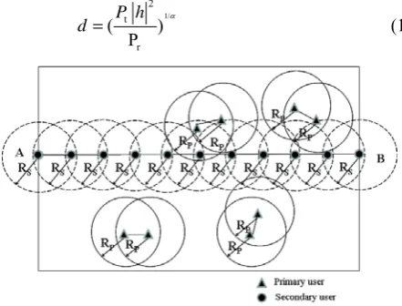
Figure 1. Model of mobile cognitive radio network.

The developed network model is illustrated in Fig. 1,

we assume the MCRN is composed of Ns mobile SUs,

stationary secondary source node A and destination node

B and Np motionless PUs. We consider a road as a line

in the model, and mobile SUs are uniformly placed along the line between A and B at the beginning. Then they move along the line between A and B based on RWP mobility model. The network size is represented with the

length L and the width D which means the distance

between A and B is L. PUs are uniformly distributed

within the cognitive radio network region.

We assume PUs and SUs are equipped with omnidirection antenna, denoting the primary

transmi-ssion range with Rp and the secondary transmission

range with Rs. The circle with radius Rp denotes the

coverage area of the PU, and the circle with radius Rs

denotes the coverage area of the SU. Now we investigate connectivity problem and only consider bidirectional links in the secondary network when we define connectivity. Therefore, when we determine whether there exists a communication link between two SUs, we need to check the existence of spectrum opportunities in both directions and the distance between these two nodes. The secondary network consists of all the SUs and all the bidirectional secondary links. As for primary network, we also consider that any primary link between two PUs is bidirectional, and a potential primary link exists between any two PUs if and only if the distance between these two

nodes is less than the primary transmission range Rp, the

primary links are illustrated in Fig. 1.

We assume that each PUj(j=1,...,Np) has a licensed

spectrum band with carrier frequency fj , denoted as

channel chj , and all the PUs transmit with a given

transmission power P, and each PUjis characterized by

an on-off transmission with activity factor βj.

ONj

j j j

ON OFF

t

t t

β =

+ (2)

where j

ON

t and j OFF

t are the average duration of the

activity period of the PU and the average duration of silence period of the PU, respectively. In addition, let Ej

represent the event that " PUj does not transmit at an

arbitrary time t ". Then the probability that this event happens is as follows.

( ) 1P Ej = −βj (3)

Each secondary user opportunistically exploits locally unused licensed spectrum without interfering

transmissions of PUs. In the same time, let Aj represent

the event that " PUj transmits at an arbitrary time t " with

probability of ( )P Aj =βj. Assuming that the events A1,

A2, …, ANp are independent and unrelated. The

probability that all the PUs are active (i.e., the probability

that all the PUstransmit at the same time) is as follows.

₁

1

( p ) p ( )

N N

active _j j j

j

p P A P A

=

=

Here we represent the interference region of a primary user as a dish of radius RPI and the interference region of

a secondary user as a dish of radius RSI(see Fig. 2). So

the behavior of a secondary link at any given time slot is dependent on two conditions: firstly, all active PUs are out of the two interference regions of the two associated SUs; secondly, these two SUs are out of the interference regions of all currently active PUs. Assuming that an active SU or PU may refer to either a transmitter or a receiver at a given time slot. Then the minimum distance between an active PU and an active SU is equal to

{

}

max ,

I PI SI

R = R R , which corresponds to the maximum

interference range, as illustrated in Fig. 2 where

PI p

R >R , RSI >Rs . To reflect the characteristic of the real wireless communication environment, we use the Log-Normal Shadowing Model [23] and assume

(6 / 5)

PI p

R = R and R_SI =(6 / 5)R_s. Notice that we define

the interference region centered at some PU or SU with

radius RI as the maximum interference region (MIR).

Therefore, a SUi can transmit by using channel chjin two

different cases:

1) when the distance between PUj and SUi is longer

than or equal to RI, SUi always identifies the channel

j

ch as unused;

2) when the distance between PUj and SUi is shorter

than RI and PUjis inactive.

If one of these two cases occurs, the channel chj is

available for the SUi.

According to the proposed network model, there are 1

s

N + segments to form the secondary network. For the

convenience of connectivity analysis, additional terms are defined as follows:

X : A continuous random variable describing the

location of a mobile cognitive node at any instant time, which represents the distribution of secondary nodes. The PDF and CDF of X are f x( )and F x( ).

x

K : A random variable denoting the length of a

segment with the left edge locating at x. The PDF and

CDF of Kx are q kx( )and Q kx( ), respectively.

i

L: A random variable denoting the location of the left

edge of the i-th segment. Let r li( ) represent the PDF of

i

L .

,

i k

p : The probability that the i-th segment has a length

shorter than or equal to k when all the PUs are inactive.

In practical application, k is a constant representing the

distance between the transmitter and the receiver.

Assuming that Rsis equal to k throughout the paper.

,

c i k

p : The probability that the i-th segment has a length

shorter than or equal to k when PUs located in the MIR

of SUi-1 or SUi are active and there is at least one

common channel between SUi-1 and SUi.

c

p : The connectivity probability of MCRN when PUs

located in the MIR of any secondary user are inactive.

c c

p : The connectivity probability of MCRN when PUs

located in the MIR of any secondary user are active.

III. CONNECTIVITY ANALYSIS

In this section, we analyze connectivity of MCRN. If

all the PUs located in the MIR of any secondary user are

inactive, SUs always have available common channel. The network composed by SUs can be considered as a traditional one dimensional mobile ad hoc network. The link between two nodes is only influenced by the distance between two nodes. Now we review an existing conventional one dimensional mobile ad hoc network connecivity analysis [5].

1

( ) [ ( )][1 ( ( ) ( ))]Ns

x s

q k =N f x+k − F x+ −k F x − (5)

where 0≤ ≤x L and 0≤ ≤ −k L x. Obviously the CDF

of Kxis as follows:

( ) 1 [1 ( ( ) ( ))]Ns

x

Q k = − − F x+ −k F x (6)

The left edge of the i-th segment will be located at l if

one node is located at l, and the remaining 2i− and

1 s

N − +i nodes are located on the left and right sides of

the node located at l, respectively. Hence, the following

equation can be obtained

1

2 2

1

( ) [ ( )] [ ( )] [1 ( )] s

s

N i

i i

i s N

r l =N f l C−₋ F l − −F l − + (7)

where 2≤ ≤i Ns+1 and 0≤ ≤l L. From (5), (6), and

(7), the probability that the i-th segment with its left edge

located at x has a length shorter than or equal to k can be

described as ( ). ( )Q k r xx i . Then pi k, is defined as

, ₀ ( ). ( ) ( )

L k L

i k x i _{L k} i

p − Q k r x dx r x dx

−

=

∫

+

∫

(8)

In (8), due to the border effect, when the left edge of a

segment falls between L−k and L , the segment is

always shorter than k , indicating a connection, i.e.

( ) 1 x

Q k = . Hence the connectivity probability in

conventional one dimensional mobile ad hoc network when the above analysis is applied becomes the following:

1

0 ,

2

( )( ) 1

0 1

s

N

i k s

i c

s

L

Q k p N

k p

L N

k

+

=

⎧ ⎡ ⎤

≥ −

⎪ _{⎢ ⎥}

⎪ ⎢ ⎥

=⎨

⎡ ⎤

⎪ _{< −}

⎢ ⎥

⎪ _{⎢ ⎥}

⎩

∏

(9)

than or equal to k, the i-th segment is considered to be

connected which means the i-th link is valid in conventional mobile ad hoc network. But the link may be invalid if there is no available channel between them in cognitive radio network. Hence, the analysis method described above must be revised.

In Fig. 2, one can see transmission range ( , )R Rs p and

interference range ( ,RSI RPI) for SU and PU,

respec-tively. To realize communication between SUi-1 and SUi,

we must consider behavior of PUs and choose channels

which are not used by PUs. This implies that the SUi-1

(SUi) can transmit data to SUi (SUi-1) if the transmission

from SUi-1 (SUi) does not interfere with nearby primary

nodes. To solve the interference problem, we consider the minimum distance between an active primary user and an

active secondary user is equal to RI =max

{

RPI,RSI

}

when we analyze the network connectivity. We can see from Fig. 2 the channel of primary link 1 is always

available to the link between SUi-1 andSUi , the primary

link 2 and the primary link 3 are not the case because of the relative location of PUs and SUs.There are two possible cases for the i-th secondary link which depend on the location of SUi-1 and SUi. Let RI < < −x L RI represent the first case of the MIR of SUi-1 or SUi being

completely within cognitive radio network region and 0≤ <x RI or L−RI ≤ ≤x L corresponds to the other case which is the MIR of SUi-1 or SUi being partly within

cognitive radio network region.

For the case of RI < < −x L RI: Fig. 2 shows SUi-1 is

located at ( ,0)x , and the MIR centered at SUi-1 is

indicated with 2

1

i I

C₋ =πR . We denote PDF of PUs with

1 ( , )

. WV

g w v

D L

= . The probability that a primary user is

located within the scope of Ci−1 is indicated with pi−1( )x .

1

2

1( ) ( , ) _.

i

I

i _C WV

R

p x g w v dA

D L

π

−

− =

∫∫

= (10)

Figure 2. Link between two neighboring SUs under influence of PUs

Similarly, SUi is located at (x+k,0), and the MIR

centered at SUi is indicated with Ci =πRI2 . The

probability that a primary user is located within Ci is

denoted with p xi( +k).

2

( ) ( , )

. i

I

i _C WV

R

p x k g w v dA

D L

π

+ =

∫∫

= (11)

Overlapping area of the MIR which is covered by SUi-1

and SUi is represented with Ccom

2 2 2

2 2

2

2 arccos

4 2

I

com I I

I

k R k

C R k R

R −

= − − (12)

The probability that all the PUs are located in the MIR

of SUi-1 or SUi is denoted with pall pu− and given by

1 0

[ ( )] [ ( )] , 1

0 , 0

p

p p

N

N j

j j

N i i p

j all pu

p

C p x wp x k N

p

N

− −

= −

⎧

+ ≥

⎪

=⎨

⎪ ₌

⎩

∑

₍₁₃₎

where, w=(Ci −Ccom) /Ci. If all the PUs are located in the MIR of SUi-1 or SUi, and all the PUs are active, the

probability that there is no available common channel between SUi-1 and SUi is given by

nc all pu active

p = p − p (14)

For the case of 0≤ <x RI or L−RI ≤ ≤x L : This

happens when not all the MIRs of SUi-1 or SUi are located

within cognitive radio network region. Notice that the probability that all the PUs are located in the MIR of SUi-1

or SUi within cognitive radio network region is different

from (13). Due to the symmetry of the model, the

analysis method of 0≤ <x RI is the same as it

of L−RI ≤ ≤x L , so we only analyze the case of

0≤ <x RI in the paper. The MIR which is covered by

SUi-1 or SUi within the scope of MCRN is denoted by

b total

C₋ and is given by

2 2 2

2 2 2

3 _{2 arcsin} 4

2 4

I

b total I I I

I

k R k

C R k R R

R

π

−

−

= + − −

(15)

The probability that all the PUs are located in the MIR

of SUi-1 or SUi within cognitive radio network regionis

b all pu

p ₋ and given by

( ) , 1

.

0 , 0

p

N b total

p b

all pu

p

C

N

p D L

N

−

−

⎧ _≥

⎪

=⎨

⎪ ₌

⎩

(16)

b

b nc all pu active

p ₋ = p ₋ p (17)

In MCRN, the link between two nearest neighboring secondary users relies on the distance and available common channel between them. If the two nodes are within the transmission range of each other and they have at least one available common channel, the link is valid, otherwise the link is noneffective. Therefore, the

connectivity probability of the i-th segment between SUi-1

and SUi is given by

, ₀ ( ) ( )

( ) ( )

( ) ( )

( ) I

I

I

I

R c

i k b nc x i

L R

nc _R x i

L k

b nc x i

L R

L

b nc i

L k

p Q k r x dx

Q k r x dx

Q k r x dx

r x dx

β β β β

−

−

−

− ₋

− ₋

=

+

+

+

∫

∫

∫

∫

(18)

where βb nc− = −(1 pb nc− ) or βnc = −(1 pnc) is the probability that there is at least one available common

channel between SUi-1 and SUi for 0≤ <x RI and

I

L−R ≤ ≤x L or R_I < < −x L R_I , respectively. The

connectivity probability of MCRN is

1

0 ,

2

( )( ) , 1

0 , 1

s

N c

i k s

i c

c

s

L

Q k p N

k p

L N

k

+

=

⎧ _{⎡ ⎤}

≥ −

⎪ ⎢ ⎥

⎪ ⎢ ⎥

=⎨

⎡ ⎤

⎪ _{< −}

⎢ ⎥

⎪ _{⎢ ⎥}

⎩

∏

(19)

The steady-state mobile cognitive users distribution of the RWP mobility model is given in [24], and the PDF and CDF is shown as follows.

2

3 2

3 2

3 2

6 6

( ) , 0

2 3

( ) , 0

f x x x x L

L L

F x x x x L

L L

⎧

= − + ≤ ≤

⎪⎪ ⎨

⎪ _{= − + ≤ ≤}

⎪⎩

(20)

Using above equations, the connectivity probability of mobile cognitive radio network can be calculated via numerical method.

IV. NUMERICAL RESULTS

Let us now verify these analytical results by computer simulation. In our simulation environment, SUs move according to the RWP model in a line, whose length and

width have been set as L=1000 ,m D=780m ,

respectively. Each secondary user picks a random spot in a line and moves there with a constant speed which is randomly chosen in [0, 5m/s]. Upon reaching this point, the node randomly picks a new destination and repeats the process. The transmission range and interference range of the PUs, whose positions are assumed static,

have been set toRp =180mand RPI =216m, respectively.

The interference range of SUs is related to transmission

range Rs . We assume any mobile cognitive node will

move towards the contrary direction at the same speed if

it reaches the border (i.e., A or B) during the sampling interval. Our simulation results are repeated 10000 times, 200 random network topologies are generated during simulation. Such the experiment is repeated 50 times for every network topology, and finally averaged over all 200 random network topologies (i.e., 10000 experiments).

Given Np =7and the activity factor of primary users

1 j

β = (j=1,...,Np), the resulting curves are shown in

Fig. 3 and Fig. 4. It may be observed that this simulation yields the same qualitative behavior as the analytical plots.

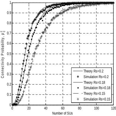
In Fig. 3, it shows simulation results are in good agreement with theoretical results for

0.15 , 0.18 , 0.2 s

R = km km km, respectively. As expected,

in all the three cases, the value of c

c

p increases with

increase of Ns for given Rs or with increase of

transmission range Rs for given Ns. One can see from

Fig. 3 that c

c

p is close to 1 when Ns is larger than 55 for

fixed Rs =200m. To reach some connectivity target

c c

p ,

the smaller the transmission range of SUs is, the more number of SUs in the secondary network is.

Fig. 4 gives the curve obtained with our formula and that produced by the simulations, we obtain the acceptable results between analytical and simulation

results. Fig. 4 demonstrates that c

c

p increases with

increase of transmi-ssion range Rs and the number of

SUs. For fixed Np, the relationship among

c c

p , Ns and S

R is similar to Fig. 3. Notice that an increase of the

transmission power of some SU leads to an increase of interference with PUs and other SUs, and the energy consumption increases accordingly. So we should take the full consideration of the tradeoff between energy

consumption and network connectivity.

Figure 3. Analytical and simulation results for different RS

0 20 40 60 80 100 120

0 0.1 0.2 0.3 0.4 0.5 0.6 0.7 0.8 0.9 1

Number of SUs

C

onnec

ti

v

it

y

P

robab

ilit

y

, p

c

c

Figure 4. Analytical and simulation results for different NS

0 2 4 6 8 10 12 14 16 18 20

0 0.1 0.2 0.3 0.4 0.5 0.6 0.7 0.8 0.9 1

Number of PUs

C

o

nn

ec

ti

v

it

y

P

rob

ab

ili

ty

, p

c

c

Theory PUs activity factor β=1 Simulation PUs activity factor β=1 Theory PUs activity factor β=0.5 Simulation PUs activity factor β=0.5 Theory PUs activity factor β=0.1 Simulation PUs activity factor β=0.1

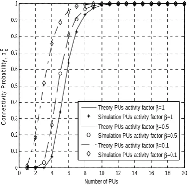
Figure 5. Number of PUs Np versus connectivity probability Pcc

Assuming Rs =0.15km , Ns =80 , Fig. 5 gives the

theoretical and simulation plots for different PUs activity

factor βj =1,βj =0.5, βj =0.1 (j=1,...,Np) , and

simulation results further verify our analysis. One can see

that the value of c

c

p increases with the increase of

number of PUs for fixed PUs activity factor, but the c

c

p

decreases with the increase of PUs activity factor βjfor

fixed Np. When the number of PUs is large enough, the

connectivity performance of MCRN is close to that of conventional mobile ad hoc network. The larger the activity factor of PUs is, the worse the network connectivity becomes. This is so because the secondary network in our model is a linear network. Increasing the number of PUs or decreasing the activity factor of PUs implies increasing the probability of available common channel between any two neighbor cognitive users.

V. CONCLUSIONS

This paper investigated the connectivity of a MCRN with RWP mobility model. We proposed a network model and derived an analytical expression which was the closed form solution of connectivity probability. We pointed out that the connectivity probability was relevant to some parameters and showed that the connectivity of the cognitive radio network was greatly impacted by the number of the PUs, the activity factor of PUs, the number of the SUs, the transmission range of the SUs, the

maximum interference range RI. Besides, increasing the

number of PUs is helpful to MCRN connectivity. A comparison is made between the theoretical analysis and simulation in various scenarios. The results derived in this paper are of practical value for researchers and developers who design MCRN or study routing of MCRN based on the connectivity probability.

ACKNOWLEDGMENT

The work was supported by National Natural Science Foundation of China (No.61172056), Doctoral Fund of Ministry of Education of China (20093201110005) from Soochow University and Jiangsu Natural Science Foundation (No. BK2011377).

REFERENCES

[1] F. Akyildiz, W. Lee, M. Vuran, and S. Mohanty, “Next generation/dynamic spectrum access/cognitive radio wireless networks: A survey,” Computer Network, vol. 50, no. 13, pp. 2127–2159, 2006.

[2] S. Haykin, “Cognitiveradio: brain-empowered wireless communica-tions,” IEEE Trans. Selected Areas in Communications, vol. 23, no. 2, pp. 201–220, 2005.

[3] M. Timmers, S. Pollin, A. Dejonghe, A. Bahai, L. V. Perre, and F. Catthoor, “Accumulative interference modeling for distributed cognitive radio networks,” Journal of Communications, vol. 4, no. 3, pp. 175-185, 2009.

[4] D. Y. Zhang, X. F. Lin, and H. Zhang, “An improved cluster-based cooperative spectrum sensing algorithm,” Journal of Computers, vol. 8, no. 10, pp. 2678-2681, 2013. [5] C. H. Foh, G. P. Liu, B. S. Lee, B. C. Seet, K. J. Wong,

and C. P. Fu, “Network connectivity of one-dimensional MANETs with random waypoint movement,” IEEE Commun. Lett., vol. 9, no. 1, pp. 31–33, 2005.

[6] M. Desai and D. Manjunath, “On the connectivity in finite ad hoc networks,” IEEE Commun. Lett., vol. 6, no. 10, pp. 437–439, 2002.

[7] J. Li, L. Lachlan, H. Andrew, C. H. Foh, M. Zukerman and M. F. Neuts, “Meeting connectivity requirements in a wireless multihop network,” IEEE Commun. Lett., vol. 10, no. 1, pp. 19–21, 2006 .

[8] P. Santi, “The critical transmitting range for connectivity in mobile ad hoc networks,” IEEE Trans. Mobile Computing, vol. 4, no. 3, pp. 310–317, 2005.

[9] C. Bettstetter, “On the minimum node degree and connectivity of a wireless multihop network,” Proc. IEEE the 3rd ACM international symposium on Mobile ad hoc networking & computing, pp.80–91, 2002.

[10]A. Abbagnale and F. Cuomo, “Connectivity-driven routing for cognitive radio ad-hoc networks,” Proc. IEEE the 7th ICC on SECON, pp. 1-9, 2010.

0 0.05 0.1 0.15 0.2 0.25

0 0.1 0.2 0.3 0.4 0.5 0.6 0.7 0.8 0.9 1

Transmission Range of SUs

C

o

nn

e

c

ti

v

it

y

P

rob

ab

il

ity

,

pc

c

[11]F. Cuomo, A. Abbagnale, and A. Gregorini, “Impact of primary users on the connectivity of a cognitive radio network,” Proc. the 9th IFIP Annual Mediterranean ad hoc networking workshop, pp. 1-8, 2010.

[12]A. Abbagnale and F. Cuomo, “Leveraging the algebraic connectivity of a cognitive network for routing design,” IEEE Trans. Mobile Computing, pp. vol. 11, no. 7, pp. 1163–1178, 2012.

[13]A. Abbagnale, F. Cuomo, and E. Cipollone, “Analysis of k-Connectivity of a Cognitive Radio Ad-Hoc Network,” ACM International Workshop on Performance Evaluation of Wireless Ad Hoc, Sensor, and Ubiquitous Networks, pp. 1-8, 2009.

[14] Q. Zhou, L. Gao, and S. G. Cui, “Connectivity of two-tier networks,” Proc. IEEE GLOBECOM Workshops, pp.368-372, 2010.

[15]P. Wang, I. F. Akyildiz, and A. M. Al-Dhelaan, “Dynamic connectivity of cognitive radio ad-hoc networks with time-varying spectral activity,” Proc. IEEE Global Telecommunications Conference, pp.1-5, 2010.

[16]W. Ren, Q . Zhao, and A. Swami, “On the connectivity and multihop delay of ad hoc cognitive radio networks,” IEEE Trans. Selected Areas in Communications, vol. 29, no. 4, pp. 805–818, 2011.

[17]W. Ren, Q . Zhao, and A. Swami, “Connectivity of heterogeneous wireless networks,” IEEE Trans. Information Theory, vol. 57, no. 7, pp. 4315-4332, 2011. [18]O. Dousse, P. Thiran and M. Hasler, “Connectivity in

ad-hoc and hybrid networks,” Proc. IEEE INFOCOM Twenty-First Annual Joint Conference of the IEEE Computer and Communications Societies Proceedings, pp.1079-1088, 2002.

[19]C. Z. Li and H. Y. Dai ,“Transport capacity and connectivity of cognitive radio networks with outage constraint,” Proc. IEEE Information Theory Proceedings IEEE International Symposium, pp.1743-1747, 2010. [20]D. Cavalcanti, N. Nandiraju, D.Nandiraju, D. P. Agrawal,

and A. Kumar, “Connectivity opportunity selection in heterogeneous wireless multi-hop networks,” Pervasive and Mobile Computing, vol. 4, no. 3, pp. 390-420, 2008. [21]K. Shafiee and V. Leung, “Connectivity-aware

minimum-delay geographic routing with vehicle tracking in VANETs,” Ad Hoc Networks, vol. 9, no. 2, pp. 131-141, 2011.

[22]K. J. Wong, “Busnet: Model and usage of regular traffic patterns in mobile ad hoc networks for inter-vehicular communications,” Proc. ICICT, pp. 1-7, 2003.

[23]L. Qin and T. Kunz, “On-demand routing in manets: The impact of a realistic physical layer model,” Proc. International Conference on Ad-Hoc, Mobile, and Wireless Networks, pp.37-48, 2003.

[24]C. Bettstetter, G. Resta, and P. Santi, “The node distribution of the random waypoint mobility model for wireless ad hoc networks,” IEEE Trans. Mobile Computing, vol. 2, no. 3, pp. 257–269, 2003.

Shuqi Liu received her B.S. degree in

School of Information Engineering from Zhengzhou University, Zhengzhou, in 2002, and M.S. degree in Electronics and Information Engineering from Soochow University, Suzhou, China, in 2005. Since 2005, she has been a lecturer at School of Electrical and Information Engineering, Jiangsu University of Technology, Changzhou, China. She is currently pursuing her Ph.D. in signal and information processing at Soochow University. Her research interests include adaptive signal processing, connectivity analysis, cross-layer design and routing design for cognitive radio networks.

Yiming Wang was born in 1956. She

received her B.S. degree in electronic device and Ph.D. degree in communications engineering from Nanjing University of Posts and Telecommunications, Nanjing, China, in 1982 and 2006 respectively. She is now a full Professor and Ph.D. supervisor at the school of Electrical and Information Engineering, Soochow University, China, where she has been leading research activities in the area of cognitive radio, multimedia communication and wireless communications. Her current research interests include communication signal processing, broadband wireless communications and cognitive radio.

Cuimei Cui received her M.A.Sc.