Differentiation of Soft Bone Strength in Human Femur Radiographic Images Using Sharpness Features and Extreme Learning Machine

(1)

International Journal of Emerging Technology and Advanced Engineering

Website: www.ijetae.com (ISSN 2250-2459, ISO 9001:2008 Certified Journal, Volume 4, Issue 6, June 2014)

777

Differentiation of Soft Bone Strength in Human Femur

Radiographic Images Using Sharpness Features and Extreme

Learning Machine

T. Christy Bobby

Department of Electronics and Communication Engineering, East Point College of Engineering and Technology, Bangalore, 560 049, India

Abstract— In this work, an attempt has been made to

analyze human femur radiographic bone images using sharpness features and learning models. The sharpness features are derived for the neck of the femur bone images to characterize the trabecular structure. The significant parameters are found using Independent component analysis (ICA) and Principal Component Analysis (PCA). The first three most significant parameters are used as inputs to the Extreme Learning Machine (ELM) and Evolutionary Extreme Learning Machine (E-ELM) classifiers and the performance of the classifiers and feature selection techniques are analysed. The results demonstrate that it is possible to differentiate normal and abnormal images using sharpness features. Also, the E-ELM classifier using radial basis activation function performs better in terms of classification accuracy (99%) for the features selected using ICA

Keywords— Evolutionary Extreme Learning Machine, Extreme Learning Machine, Human femur, Independent Component Analysis, Principal Component Analysis, Sharpness features, Trabecular structure.

I. INTRODUCTION

Osteoporosis is characterized by a loss of bone mass and a deterioration of the trabecular structure. Bone strength reflects both bone density and quality. Bone quality depends on trabecular architecture, mineralization, turnover, and micro-fracture accumulation. The potential benefits from trabecular architecture evaluation would be expected to improve the prediction of the fracture. Radiographs are commonly used to quantify trabecular texture patterns in human femur bones. The significant parts of the information that are available in 3D images are also available in the conventional radiographs. Trabecular bone structure is also visible in great detail on standard radiographs [1, 2]. Hence, there has been considerable interest in using conventional radiography combined with various image and texture analysis techniques for assessing trabecular structure.

Conventionally, radiologists perceive image patterns and diagnose on the basis of a combination of their training, experience, and individual judgment.

It follows that there will be an inevitable degree of variability in image interpretation as long as it relies primarily on human visual perception. Hence tools for automated image analysis system can provide objective information to support clinical decision-making and may serve to reduce this variability [3]. Texture characterization of the images is an important part in medical image analysis. Texture analysis describes a wide range of techniques that enable quantification of the gray-level patterns, pixel interrelationships, and the spectral properties of an image that are imperceptible to the human visual system [3, 4].

One of the techniques used to inspect textural abnormalities is calculation of image sharpness features. The sharpness features are categorised in to four categories, which include derivative based, statistical based, histogram based and transforms based parameters. Derivative based parameters give scale-space representation of the image. Statistical texture analysis methods measure the spatial distribution of pixel values. Despite their simplicity, histogram techniques are invariant to translation and rotation, and insensitive to the exact spatial distribution of the pixels. Transform based parameters are based on the ratio of upper to lower spatial frequency energy. Two-dimensional transforms have been used extensively in image processing to tackle problems such as image description and enhancement. Texture directionality preserved in the power spectrum allows directional and non-directional components of the texture to be distinguished. These characteristics make them ideal for medical image discrimination applications. In the literature, the sharpness features are used to find the focus characteristics of the microscopy images. [5, 6]. In this work the sharpness features are used to distinguish the trabecular architectural variation in the femur bone images.

(2)

International Journal of Emerging Technology and Advanced Engineering

778

In the analysis of multivariate dataset, PCA finds a set of the most representative projection vectors such that the projected samples retain most of the information about original samples. ICA captures both second and higher-order statistics and projects the input data onto the basis vectors that are as statistically independent as possible [7, 8].

Artificial Neural Networks (ANN) have seen a rapid growth and it has been applied widely in many biomedical applications such as human facial expression recognition [9], automatic detection of breast cancer [10] and multiple objective decision making problems [11]. The Extreme Learning Machine (ELM) is a neural network algorithm proposed recently as an efficient learning algorithm for Single-hidden Layer feed Forward Neural network (SLFN). This method makes the selection of the weights of the hidden neurons very fast using Moore-Penrose (MP) generalized inverse problem. Also, MP avoids many difficulties faced by gradient-based learning methods such as stopping criteria, learning rate, learning epochs, and local minima. However, ELM usually needs higher number of hidden neurons due to the random determination of the input weights and hidden biases [12]. Evolutionary Extreme Learning Machine (E-ELM) has been proposed by taking advantages of both ELM and Differential Evolution (DE) to remove redundancy among hidden nodes and achieve satisfactory performance with more compact networks [13].

In this work, the sharpness features are derived for the human femur bone X-ray images to characterize the trabecular structure. The significant parameters are found using feature selection techniques such as ICA and PCA. The first three most significant parameters are used as inputs to the ELM and E-ELM classifiers. The performance of the classifiers and feature selection techniques are analyzed using classification accuracy.

II. METHODOLOGY

An easy way to comply with the conference paper formatting requirements is to use this document as a template and simply type your text into it. Digitized pelvis images (N = 60, normal= 21, abnormal 39) recorded using clinical X-ray unit are considered for this analysis. Auto threshold algorithm is employed to recognize the presence of mineralization in the digitized images [14]. From the pre-processed bone images, Region of Interest (ROIs) of image size 163 × 163 pixels are chosen from the femoral neck. The femoral neck region is selected for the analysis, as clear trabecular architecture and architectural variations are seen in this region due to stress distribution.

The ROIs is selected in such a way that it covers the upper region of the neck lying on the principal tensile trabeculae, the lower region of the neck lying at the base of the principal compressive trabeculae and Ward's Triangle lying between these structures [15, 16].

The sharpness features [5] are extracted for both normal and abnormal femur bone images. Derivative based parameters (d1- d6) obtained for the analysis include squared gradient, Brenner gradient, Tenenbaum gradient, energy Laplace, contrast and sum of squared Gaussian derivatives. Statistical parameters (s7-s10) derived are variance, normalized variance, autocorrelation and standard deviation based correlation. Image histogram based parameters (h11-h15) estimated are range algorithm, threshold content, threshold pixel count, image power and entropy. Image transform based parameters (t16, t17) derived are Shen and Chen’s algorithms and AC energy based focus measure. These parameters are examined to distinguish normal and abnormal bone images. The most significant features are extracted using feature selection algorithms and those features are employed for classification to achieve better performance.

The Principal Component Analysis is performed on the features derived. PCA uncovers combinations of the original variables which describe the dominant patterns and the main trends in the data. This is done through an eigenvector decomposition of the covariance matrix of the original variables. The extracted latent variables are orthogonal and they are sorted according to their eigenvalues. The high dimensional space described by matrix X is modelled using PCA as

T

X TP E (1) Where T is the score matrix composed by the principal components, P is the loadings composed by the eigenvectors of the covariance matrix and E is the residual matrix[17].

The ICA is also performed on the derived feature set. Let s be the vector of unknown source signals and Y is the vector of observed mixtures. If A is the unknown mixing matrix, then the mixing model is written as

Y



As

(2)

(3)

International Journal of Emerging Technology and Advanced Engineering

779

u



Wx



WAs

(3)

is an estimation of the independent source signals[18]. The three most significant parameters derived using PCA and ICA are used as input feature vectors to the classifiers. Training SLFNs with K hidden neurons and activation function g(x) is used to learn N distinct

samples ( , )x t_i _i , where x_i [x_i₁,x_i₂,...,x_in]T Rn is

the inputs and t_i [t_i₁,t_i₂,...,t_im]T Rm is the targets. In ELM, the nonlinear system has been converted to a linear system:

H





T

(4)

Where H 

 

h_ij (i1, ...,N and j 1, ...,K) is the

hidden-layer output matrix, h_ij_g w( _j.x_ib_j) denotes the

output of jth hidden neuron with respect to

x

_i

, [ 1, 2..., ]

T

j j j jn

w  w w w

is the weight vector connecting jth

hidden neuron and input neurons, and

b

j denotes the bias of jth hidden neuron; w x_j. _i denotes the inner product of

j

w

, [ 1, 2..., ]

T k

   

is the matrix of output weights

and _j [ _j₁, _j₂...,_jm] (T j 1, ..., )k denotes the

weight vector connecting the jth hidden neuron and output neurons; T [ ,t t₁ ₂,...,t₃]T is the matrix of targets .Thus, the determination of the output weights is as simple as finding the Least-Square (LS) solution to the given linear system. The minimum norm LS to the linear system is

† , H T

 

 (5)

Where H† is the MP generalized inverse of matrix H. The minimum norm LS solution is unique and has the smallest norm among all. In E-ELM using DE and MP generalized inverse, the population is randomly generated.

The population is composed of a set of input weights and hidden biases.

,

, ...,

,

, ...

,... ,

,

11 12

1 21 22

2

1 ,...

,...

,

,...,

2

1

2 w

w

k

n

w

b

n

nk

k



_

















(6)

All wij and bj are randomly initialized within the range of

[−1, 1]. For each individual the corresponding output weights are analytically computed by using the MP generalized inverse. The fitness of each individual is evaluated using cost function (E) is Root Mean Squared Error (RMSE)

2

( . )

1 1 ₂

N K _{g W} _X _b _t

i i j i j

j i

E

m N

  

 _  _

 (7)

The fitness to the RMSE only on the validation set is used to save time. After the fitness, all individuals in the population are calculated in three steps of DE are: mutation, crossover and selection. In DE, during selection, the mutated vectors are compared with the original ones, and the vectors with better fitness values are retained to the next generation. However, for neural networks training, using the fitness alone as the selection criteria is not appropriate. Therefore, to further improve the generalization performance, one more criteria is added into

the selection: the norm of output weights  . In this

selection strategy, when the difference of the fitness between different individuals is small, in that the smaller

 is selected. The determination of new

population



_i

,

_G_₁, can be described as follows

, ( _, ) ( _, ) ( _, ),

, ( _, ) ( _, ) ( _, ) ( _, )

, ₁

, ,

,

, ,

G if f f f

i i G i G i G

G if f f f f

i i G i G i G i G

and i G

i G i G

else i G

    

      



 

 



 

  

 













(8)

(4)

International Journal of Emerging Technology and Advanced Engineering

780

The TP and TN are the cases where the abnormal is classified as abnormal and normal classified as normal, respectively [20].

III. RESULTS AND DISCUSSION

Typical pre-processed radiographic images of normal and abnormal femur trabecular bones are shown in Figures 1 (a) and (b) respectively. The trabecular patterns are found to be closely arranged in normal images, whereas the trabecular spacing is seen with discontinuities in abnormal cases. The overlap between trabeculae is also found to be less in abnormal images. The ROI selected for analysis is shown in Figures 1 (c)

(a) (b)

100 200 300 400 500 600 700 800 100

200

300 400

500 600

700 800

900

[image:4.612.326.570.170.403.2]

(c)

Fig. 1. Typical normal (a) abnormal (b) and ROI (c) femur bone images

The normalized average and standard deviation values of the derived sharpness features for ROI femur images are shown in table 1. It is observed from the results that the mean values of the d1, d2, d3, d4, d5, d6, s9, s10, h11, h12, h13, h14, h15 features are found to be distinct for normal and abnormal images. This is likely attributable to prominent trabecular architecture and architectural variations seen in the selected ROI. Some features are not highly distinguishable as the mean values are nearly the same.

Table 1.

Normalized average and standard deviation values of thederived sharpness parameters for ROI

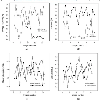
Figure 2(a) and (b) show the variation of energy Laplace and contrast features for various images. These two features are found to have clear demarcations between normal and abnormal images. Where, the squared gradient and Variance features shown in figures 2(c) and (d) respectively have overlapping values for normal and abnormal images. This raises an ambiguity in employing all the features for classification procedure, as it increases the complexity of the classifier. Thus the most significant features are extracted using feature selection algorithms and those features are employed for classification to achieve better performance.

To reduce the complexity in classifying the normal and abnormal images, the features are selected using PCA and ICA. The significant feature vectors are sorted by the magnitude of variance using PCA and kurtosis using ICA. The first three significant features selected using PCA are Energy Laplace (d4), Entropy (h15) and Threshold content (h12). The features selected using ICA is Brenner gradient (d2), Energy Laplace (d4) and Range algorithm (h11).

Sharpness features Normal Abnormal Squared gradient (d1) 0.41±0.13 0.29±0.01 Brenner gradient (d2) 0.53±0.23 0.35±0.11 Tenenbaum gradient (d3) 0.55±0.56 0.41±0.53 Energy Laplace (d4) 0.72±0.38 0.36±0.26 Contrast (d5) 0.73±0.37 0.35±0.24 Sum of squared Gaussian

derivatives (d6) 0.72±0.38 0.36±0.26 Variance (s7) 0.51±0.16 0.51±0.14 Normalized variance (s8) 0.46±0.38 0.46±0.05 Autocorrelation (s9) 0.52±0.003 0.43±0.35 Standard deviation

based correlation (s10) 0.59±0.32 0.46±0.25 Range algorithm (h11) 0.72±0.707 0.44±0.21 Thresholded content (h12) 0.72±0.34 0.59±0.22 Thresholded pixel count (h13) 0.51±0.25 0.54±0.33 Image power (h14) 0.64±0.28 0.49±0.25 Entropy (h15) 0.91±0.02 0.93±0.04 AC energy algorithm (t16) 0.51±0.16 0.51±0.14 Shen and Chen’s algorithm

[image:4.612.68.277.291.531.2]

(5)

International Journal of Emerging Technology and Advanced Engineering

781

0 5 10 15 20

0.0 0.1 0.2 0.3 0.4 0.5 0.6 0.7 0.8 0.9 1.0

Normal Abnormal

E

n

e

rg

y

la

p

la

c

e

[

d

4

]

Image Number

0 5 10 15 20

0.0 0.1 0.2 0.3 0.4 0.5 0.6 0.7 0.8 0.9 1.0

Normal Abnormal

C

o

n

tr

a

st

[

d

5

]

Image number

(a) (b)

0 5 10 15 20

0.0 0.2 0.4 0.6

Normal Abnormal

S

q

u

a

re

d

g

ra

d

ie

n

t

(d

1

)

Image number

0 5 10 15 20

0.1 0.2 0.3 0.4 0.5 0.6 0.7 0.8 0.9

Normal Abnormal

V

a

ri

a

n

c

e

(

s

7

)

Image Number

[image:5.612.139.505.127.477.2]

(c) (d)

Fig. 2. Scattergram of (a) Energy Laplace (b) Contrast(c) Squared gradient (d) Variance value for normal and abnormal images

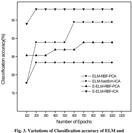
The optimal feature reduction technique among PCA and ICA is analyzed based on the performance of the classifier. These significant features are given as inputs to the ELM and E-ELM classifiers for further analysis. Table 2 shows the accuracy of classification models with different activation functions such as Sigmoidal, Sine, Hardlim, Triangular basis (TBF) and Radial Basis Functions (RBF). Figure 3 shows the comparison between the classification accuracy of the ELM and E-ELM classifier for features selected using PCA and ICA for varying number of epochs.

[image:5.612.332.556.521.665.2]

Features selected by ICA produced a maximum classification accuracy of 94% for hardlim activation function from 600 epochs using ELM classifier. The features selected using PCA produced only 83% of maximum classification accuracy using RBF activation function from 200 epochs for the same classifier.

Table 2.

Accuracy of ELM and E-ELM for different activation functions for PCA and ICA

Activation function

Accuracy (%)

ELM E-ELM

PCA ICA PCA ICA

Sigmoidal 77 77 77 94

Sine 77 77 83 94

Hardlim 61 94 83 94

TBF 55 83 83 94

RBF 83 66 88 98

(6)

International Journal of Emerging Technology and Advanced Engineering

782

The maximum classification accuracy is found to be 88% for RBF function from 700 epochs for features selected using PCA.

The results show that both the classifiers show better classification efficiency for ICA selected features. Also, the classification accuracy of E-ELM classifier for ICA selected features is much higher and settles at a maximum value for less number of epochs compared to all the cases. This may be due to the fact that ICA features are sorted based on the kurtosis value which describes the peakedness in the data set. The main advantage of using kurtosis is its computational simplicity. Also, the selected features are Gaussian random variables, independent and they are uncorrelated with each other.

100 200 300 400 500 600 700 800 900 1000 1100 75

80 85 90 95

ELM-RBF-PCA ELM-hardlim-ICA E-ELM-RBF-PCA E-ELM-RBF-ICA

C

la

s

ifi

ca

tio

n

a

cc

u

ra

cy

(%

)

[image:6.612.52.284.303.537.2]

Number of Epochs

Fig. 3. Variations of Classification accuracy of ELM and E-ELM

Thus it is observed from the results ICA based feature reduction technique with E-ELM model using RBF performs efficiently in terms of accuracy (98%) and lesser number (200) of epochs. As it takes lesser number of epochs, for the classification the training and testing time is considerably reduced. The method helps in differentiating normal and abnormal images efficiently based on a feature selection technique which includes features that are uncorrelated in nature.

IV. CONCLUSION

Characterization of trabecular bone quantity and quality has received considerable attention due to its sensitivity to hormonal, mechanical, and therapeutic effects. In this work, sharpness features are derived to characterize normal and abnormal trabecular femur bones using conventional radiographs. Estimation of sharpness features have been attempted for the first time in trabecular images as per the author’s knowledge. Among the seventeen features, thirteen features showed differentiation of normal and abnormal images in terms of their mean values. The results demonstrate that it is possible to differentiate normal and abnormal images using sharpness features. Also it is seen that the E-ELM classifier uses RBF activation function showing better classification accuracy (98%) for features selected using Independent component analysis. Hence it appears that characterization of femur image using sharpness features could be used as an index for automated image analysis system and gross abnormality detection, micro-damage studies and modelling the mechanics of soft tissue in diseases.

REFERENCES

[1] Lespessailles, E., Chappard, C., Bonnet, N., Benhamou, C.L. (2006). Imaging Techniques for Evaluating Bone Microarchitecture. Joint Bone Spine, 73, 254–261.

[2] Donnelly, E. (2011). Methods for Assessing Bone Quality a Review. Clin Orthop Relat Res, 469, 2128–2138.

[3] Kassner, A., Thornhill, R.E (2010). Texture Analysis: A Review of Neurologic MR Imaging Applications. Am J Neuroradiol, 31, 809– 816.

[4] Xie, X. (2008). A Review of Recent Advances in Surface Defect Detection using Texture analysis Techniques. ELCVIA, 7(3), 1-22. [5] Artyukhova, O.A., Samorodov, A.V. (2011). Comparative Study of

Sharpness Parameters of Microscopic Images of Biomedical Preparations. Biomed. Engg, 45(1), 12-18.

[6] Nailon, W.H. Texture Analysis Methods for Medical Image Characterisation. Biomedical Imaging, 75-100.

[7] Kavitha, A., Sujatha, M., Ramakrishnan, S. (2011). Evaluation of Flow–Volume Spirometric Test Using Neural Network Based Prediction and Principal Component Analysis. J Med Syst, 35, 127– 133.

[8] Cai, L., Tian, X. (2011). Improved Post-Nonlinear Independent Component Analysis Method Based on Gaussian Mixture Model. In: Fourth International Workshop on Advanced Computational Intelligence, pp.19-21.

(7)

International Journal of Emerging Technology and Advanced Engineering

783 [10] Elif, D.U. (2009). Adaptive Neuro-Fuzzy Inference Systems for

Automatic Detection of Breast Cancer. JOMS, 33(5), 353-358. [11] Cheng, C., Cheng, C.J., Lee, E.S. (2002). Neuro-Fuzzy and Genetic

Algorithm in Multiple Response Optimization. Appl. Comput. Math, 44, 1503-1514

[12] Liu, N., Wang, H. (2010). Ensemble Based Extreme Learning Machine. IEEE Signal Process Lett. 17(8), 754-757.

[13] Huynh, H.T., Won, Y. (2009). The Use of Evolutionary Algorithm in Training Neural Networks: Evolutionary Computation, Evolutionary Computation, Book edited by: Wellington Pinheiro dos Santos, ISBN 978-953-307-008-7, pp. 572, October 2009, I-Tech, Vienna, Austria.

[14] Christopher, J.J., Ramakrishnan, S. (2008). Assessment and classification of mechanical strength components of human femur trabecular bone using texture analysis and neural network. J Med Syst, 32(2), 117–122

[15] Gregory, J.S., Stewart, A., Undrill, P.E., Reid, D.M., Aspden, R.M. (2004). Identification Of Hip Fracture Patients From Radiographs Using Fourier Analysis Of The Trabecular Structure: A Cross-Sectional Study. BMC Med Imaging, 4(4), 4-14.

[16] Rudman, K.E., Aspden, R.M., Meakin, J.R. (2006). Compression or tension? The stress distribution in the proximal femur. Biomed Eng Online. 5(12).

[17] Aguado, D., Montoy, T., Borras, L., Seco, A., Ferrer, J. (2008): Using SOM and PCA for analyzing and interpreting data from a P-removal SBR. Eng. Appl. Artif. Intell, 21, 919-930 .

[18] Draper, B.A., Baek, K., Bartlett, M.S., Beveridgea, J.R. (2003). Recognizing Faces with PCA and ICA. Comput. Vision Image Understanding. 91, 115-137.

[19] Zhu, Q., Qin, A.K., Suganthan, P.N., Huang, G.B.: Evolutionary Extreme Learning Machine. Pattern Recognit. 38, 1759-1763 (2005) [20] Fawcett, T.: An introduction to ROC analysis. Pattern Recognit. Lett.