© 2017, IRJET | Impact Factor value: 5.181 | ISO 9001:2008 Certified Journal
| Page 479
Performance Comparison of Sensor Deployment Techniques
Used in WSN
R.S.Kittur
1, A.N.Jadhav
21
D.Y. Patil College of Engineering & Technology, Kolhapur,Maharashtra, India
2
D.Y. Patil College of Engineering & Technology, Kolhapur, Maharashtra, India
---***---
Abstract -Wireless Sensor Networks consisting of nodeswith limited power and are deployed to gather useful information from the field. In WSN, it is critical to collect the information in an efficient manner. When nodes are randomly deployed, all the nodes may not be used efficiently which will reduce the network lifetime. In this paper, we implement artificial bee colony algorithm for proper deployment of sensor nodes and calculate network lifetime in terms of upper bound for this configuration. Simulation results prove that compare to random and heuristic deployment, artificial bee colony performs better for providing enhanced network lifetime.
Key Words:Wireless sensor network, Deployment, Scheduling, Upper Bound, Network Lifetime.
1.INTRODUCTION
1.1 Wireless Sensor Network:
Wireless sensor network is nothing but collection of huge numbers of sensor nodes. Each sensor node consists of sensors, actuators, memory unit and transceivers. Coverage and network lifetime are the basic two crucial problems associated with wireless sensor network and on which we are focusing in this paper. Coverage needs to guarantee that all the targets in area of interest should be monitored with required degree of reliability. In general, coverage answers the questions about quality of service (surveillance) that can be provided by a particular sensor network. In target coverage, there are several points of interest in a given region and sensors need to cover all the points. Sensors collect the data by monitoring the targets in their sensing ranges. With the current available technology, sensors are battery powered. Due to the limitation of battery, how to prolong the network lifetime is a critical issue in wireless sensor networks. For coverage problems, lifetime is the time duration that all the targets or the area is continuously covered. There are two main modes of sensor radio in the network, active and sleep. Sleep means a sensor radio is turned off without any activities while active means the radio is turned on and the active sensors can sense the environment surrounding them. One sensor can only be in one mode at a time. The power consumption of sleep mode is 0.03W much less than that of active mode which
varies between 0.38W-0.7W. In this paper, we are implementing artificial bee colony algorithm for deployment of sensor nodes in wireless sensor network and comparing its result with random and heuristic deployment techniques.
1.2 Sensor Node Deployment
:
Deployment of node is nothing but placement of sensor node in monitoring area. Deployment maybe random deployment or deterministic deployment.Random deployment
: Random deployment is suitable for applications where the details of the regions are not known, or regions are inaccessible. An example of random deployment of sensor nodes would be in battlefield surveillance. In such a deployment, the most common way of extending the network lifetime is by scheduling the sensor nodes such that only a subset of sensor nodes that is enough to satisfy coverage requirement need to be active at a time.Deterministic deployment
:
In deterministic deployment, the details of the region will be known a priori and a provision of deploying nodes at specific locations is possible. As nodes are deployed at particular locations, this method provides better target coverage.1.3 Coverage in WSN
:
Each target in area to be monitored should be monitored continuously by at least one sensor node that is target should be in the sensing range of sensor node. Such network provides required degree of coverage and performs the task in proper way for which it is used.© 2017, IRJET | Impact Factor value: 5.181 | ISO 9001:2008 Certified Journal
| Page 480
sensor nodes can be scheduled to achieve the optimumlifetime. Sensor deployment and scheduling in this way contributes equally to extend the network lifetime. In [8], authors use the ABC algorithm for the deployment of sensors nodes in the network to obtain good coverage in a 2-dimensional space.
2. Network Lifetime Upper Bound in WSN:
It is a parameter calculated mathematically and used for comparison of different deployment algorithms going to implement.
Assume m number of sensor nodes as S1, S2, . . . , Sm which are randomly deployed to cover the region with dimension as X by Y. These m number of sensor nodes monitors then targets as T1, T2, . . . , Tn.
Each sensor node has an initial energy Eo and a sensing radius Sr. A sensor node Si, 1 ≤ i ≤ m, is said to cover a target Tj, 1 ≤ j ≤ n, if the distance between Si and Tj is less than Sr . The coverage matrix is defined as,
1 if Si monitors Tj……..(1) Mij =
0 otherwise where i = 1, 2, . . . ,m.
j = 1, 2, . . . , n.
Now consider initial battery power as bi and energy consumption rate of each node as ei and thus
bi’ = bi / ei represents the lifetime of battery in terms of time. By using above data, the upper bound is calculated as,
∑
………….(2)
For k-coverage,
q j= k, j = 1, 2, . . . , n.
The upper bound is the maximum achievable network lifetime for a particular configuration.
3
. PROPOSED METHOD :
Proposed method consist of implementation of Artificial bee colony (ABC) algorithms and comparison of results of ABC algorithm with random deployment and heuristic deployment algorithm.
3.1 Random Deployment:
Large number of sensor nodes are placed randomly in the area to be monitored which is not accessible easily. Random deployment affects the network life in WSN because this deployment method does not provide required degree of coverage.
3.2 Heuristic Deployment:
One of the approaches of dynamic deployment of sensor nodes in WSN used to enhance network lifetime of WSN. This method gives efficient results compared with random deployment. In this technique, a sensor is moved in such a way that it should cover large number of targets. So that large number of cover sets can be formed. For that, initially place all nodes randomly and move any idle node to least monitored node. Now move all nodes at the center of targets it covers. Further, nearest target is to be identified and node is again placed at the middle of these entire targets. If node can covers this new target also then node is allowed to move else discard this move and finally calculate the upper bound. The performance of Heuristic deployment is understood by flowchart given in fig 1.
Fig.1 Flowchart for Heuristic Deployment
3.3 Artificial Bee Colony Based Deployment:
This optimization algorithm is based on intelligent behavior of Honey Bee Swarm. Here sensors are placed, where large numbers of targets are placed so that each target is covered by large number of sensors. In this algorithm, initially all the targets are covered such that each node at least covers one target and network lifetime is calculated using equation (2).
© 2017, IRJET | Impact Factor value: 5.181 | ISO 9001:2008 Certified Journal
| Page 481
the initial position of ith cluster. F (Di)refers to the nectaramount at food source located at Di. After watching the waggle dance of employed bees, an onlooker goes to the region Di where large numbers of targets are present with probability pidefined as,
Pi = ∑
……..(3)
wherem is the total number of food sources. The onlookerfinds a neighborhood food source in the vicinity of Di as,
Di (t + 1) = Di (t) + δij× f ……….. (4)
Where δij is the neighborhood patch size for jth
dimension of ith food source, and f is a random uniform
variate ∈[−1, 1].
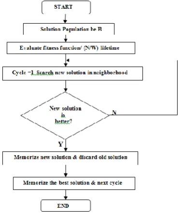
It should be noted that the solutions are not allowed to move beyond the edge of the search region. The new solutions are evaluated using the fitness function (2). If any new solution is better than the existing one, the old solution is replaced with new solution. Scout bees search for a random feasible solution. The solution with the least sensing range is finally selected as best solution. Concept of ABC deployment algorithm flowchart is given in fig 2.
Fig 2. Flowchart for ABC Deployment
4. SIMULATION RESULTS
Simulation for analyzing performance of random, heuristic and ABC deployment is carried first on 300m x 300m region area and then varied to 400m X 400m. For both region areas, comparative results of ABC with random and heuristic deployment are obtained by
[image:3.595.75.262.419.642.2]changing following parameters. Simulation is carried out using Matlab1012a.
Table -1: Specification Table Sr.
No. Specification Value
1 Region area 300m X 300m and
400m X 400m
2 Number of Targets 30, 40 and 50
3 Number of sensor node 50,100, 150
4 Sensing Range 30m to 50m
5 Sensor node battery
power 1000 units
Case I: Performance analysis for change in number of sensor nodes.
Number of Targets = 25
Sensing range of sensor node = 50m
Chart -1: Effect of change in sensor nodes
Chart -2: Effect of change in sensor nodes
50 100 150
0 200 400 600 800 1000 1200 1400 1600 1800 2000
Number of Sensor Nodes
N
e
tw
o
rk
L
if
e
T
im
e
Region area 400m x 400m
Random Heuristic ABC
50 100 150
0 1000 2000 3000 4000 5000 6000
Number of Sensor Nodes
N
e
tw
o
rk
L
if
e
T
im
e
Region area 300m X 300m
© 2017, IRJET | Impact Factor value: 5.181 | ISO 9001:2008 Certified Journal
| Page 482
Case II : Performance analysis for change in coverage(sensing) range of sensor nodes as 30m, 40m and 50m. Number of sensor nodes = 100
Number of Targets = 25
Chart -3: Effect of change in sensing range
Chart -4: Effect of change in sensing range
Case III: Performance analysis for change in target nodes.
Number of sensor nodes = 100 Sensor node coverage range = 50m
Chart -5: Effect of change in target nodes
Chart -6: Effect of change in target nodes
Table -2: Effect on network lifetime for 20m sensing range
Sr. No.
Area (Sq. meter)
Range (meter)
No.of Sensor s
No.of Targe ts
Network Lifetime
Random Heuris
tic ABC
1 100 20 50 25 298 1226 5054
2 150 20 50 25 299 887 2635
3 200 20 50 25 280 554 868
4 250 20 50 25 274.6 588 658
5 250 20 75 25 279.6 896 2454
6 250 20 100 25 304 1122 3320
6. RESULT DISCUSSION
Performance of ABC is definitely better compare to random and heuristic deployment which is shown in all
30 40 50
0 500 1000 1500 2000 2500
Change in coverage range (m)
N
e
tw
o
rk
L
if
e
T
im
e
Region area 400m x 400m
Random Heuristic ABC
30 40 50
0 500 1000 1500 2000 2500 3000 3500 4000 4500 5000
Change in coverage range (m)
N
e
tw
o
rk
L
if
e
T
im
e
Region area 300m x 300m
Random Heuristic ABC
30 40 50
0 500 1000 1500 2000 2500
Number of Target Nodes
N
e
tw
o
rk
L
if
e
T
im
e
Region area 400m x 400m Random Heuristic ABC
30 40 50
0 500 1000 1500 2000 2500 3000 3500 4000 4500
Number of Target Nodes
N
e
tw
o
rk
L
if
e
T
im
e
Region area 300m x 300m
© 2017, IRJET | Impact Factor value: 5.181 | ISO 9001:2008 Certified Journal
| Page 483
charts. It is the improvement in one of the quality factorof wireless sensor network by using such techniques for deployment of sensor nodes in WSN.
Also simulation results shows that by changing different parameters of WSN, performance of ABC deployment algorithm is more and more efficient compare to basic random and heuristic deployment algorithm.
When region area is increases while keeping other parameters of WSN remains constant, then network lifetime reduces as shown in all three cases. As region area increases, sensor nodes dispersed more when deployed. So number of sensor nodes covering a target goes on reduces. Due to that cover sets providing required coverage also go on reduces, which affects the network lifetime.
When numbers of sensor nodes are increases in constant region area, definitely network lifetime enhances shown in case I. As in this situation, there is chance of more number of sensor nodes will cover a target. Because of that large number of cover sets will form. When more number of cover sets are there in WSN, then during scheduling it will improve the network lifetime.
The same results will obtained when sensing range of sensor nodes is increases. Because as sensing range of sensor node increases, more number of near most targets may come in the range sensor node. So case II shows that improvement in network lifetime with increase in sensing range of sensor node.
When numbers of target nodes are increases while keeping other parameters constant, network lifetime reduces as shown results in case III. Because same number of sensor nodes should sense the information continuously and transmit that to the base station from all the targets as go on increases.
Table 1 again shows the effect on network lifetime. Sr. no. 4 and sr. no 6, if compare then it is clear that in same area if numbers of sensors are doubled then network lifetime is approximately five times more for ABC deployment algorithm. By analyzing such comparison, it is easy to select the network parameters depending on the requirement of application.
7.
CONCLUSION
In this paper, we analyze the performance of random, Heuristic and Artificial Bee Colony deployment algorithms. Network survives for more time if ABC algorithm is used for deployment of sensor nodes in wireless sensor network. Even if different parameters of WSN are changed compare to other deployment, ABC deployment algorithm outperforms in all situations. Future work is performance study of scheduling algorithms with dynamic deployment for improvement of network lifetime with required level of target coverage.
REFERENCES:
[1] K. Kar and S. Banerjee, “Node placement for connected coverage in sensor networks”, in Proc. Model.
Optim. Mobile, Ad Hoc Wireless Netw.,2003, pp.556–563.
[2] V. Raghunathan. C. Schurgers, S. Park, and M. B. Srivastava , “Energy-Aware Wireless Micro sensor Networks”, IEEE Signal Processing Magazine.19 (2002), pp.40-50
[3] S. Mini, Siba K. Udgata, and Samrat L. Sabat” Sensor Deployment and Scheduling for Target Coverage Problem in Wireless Sensor Networks”, IEEE SENSORS JOURNAL,VOL.14, NO. 3, MARCH 2014
[4] K. Dasgupta, M. Kukreja, and K. Kalpakis, “ Topology-aware placement and role assignment for energy-efficient information gathering in sensor networks”, in
Proc. IEEE ISCC, 2003, pp. 341–348.
[5] T. Nieberg, J. Hurink, and W.Kern, “Approximation schemes for wireless networks” ,ACM Trans .Algorithms, vol. 4,no. 4, pp. 49:1–49:17, Aug. 2008.
[6] M. Cardei, M. T. Thai, Y. Li, and W. Wu, “Energy-efficient target coverage in Wireless sensor networks” ,
in Proc. 24th Annu. Joint Conf. IEEE INFOCOM, Mar. 2005,
pp. 1976–1984.
[7] S. Mini, S. K. Udgata, and S. L. Sabat,“Sensor deployment in 3-D terrain using artificial bee colony algorithm”, in Proc. Swarm, Evol. Memetic Comput., 2010, pp. 424–431.
[8] C. Ozturk, D. Karaboga, and B. Gorkemli, “Artificial bee colony algorithm for dynamic deployment of wireless sensor networks” ,TurkishJ. Electr. Eng. Comput. Sci., vol. 20, no. 2, pp. 255–262, 2012.
[9] S. Mini, S. K. Udgata, and S. L. Sabat, “Artificial bee colony based sensor deployment algorithm for target coverage problem in 3-D terrain”, in Proc. Distrib.