Maximizing Wireless Sensor Network Lifetime based on Linear Programming Method

(1)

Maximizing Wireless Sensor Network Lifetime Based on Linear

Programming Method

Farzad Kiani

Department of Computer Engineering, Engineering and Natural Sciences Faculty, Istanbul Sabahattin Zaim

University, 34303, Istanbul, Turkey

---*---Abstract**

- The wireless sensor network (WSN) is a distributed, self-organizing network of a set of sensors designed to track physical phenomena or environmental conditions. By relaying messages from one element to another, the coverage area of such a network can reach several kilometers. In this paper, a uniform distribution has been used to distribute several nodes (sensors) within a circular area, all the used nodes with the same initial energy. The main problem of WSN is the gradual depletion of energy during the process of transferring data from one node to another down to the manager node (base station). The goal of this paper is to maximize the lifetime of the wireless network as much as possible by using one of the optimization techniques called linear programming (LP). The proposed system has been tested and implemented by using General Algebraic Modeling System (GAMS).

Key Words:

Wireless Sensor Network, Uniform

Distribution, Linear Programming, Global Algebra Model System, Lifetime.

1. INTRODUCTION

Today, the term "wireless sensor network" is understood as wireless mesh networks with low data rate and ultra-low power consumption, which can be used not only to collect readings from sensors, but also to transmit information of another type (for example, control commands). Such networks have many practical advantages with respect to wired systems. For example, they no need to lay cables for power supply and data transmission. Low cost of installation, commissioning and maintenance of the system, minimum restrictions on accommodation wireless devices, the possibility of introducing and modifying the network operated object without intervention in the process of functioning are other their properties. In addition, reliability and fault tolerance of the entire system is better if it is compared to wired systems.

The wireless communications in wireless sensor networks (WSN) are popular in last year’s [1]. They are different from the other wireless networks such as Mobile Ad-hoc Network so they are combining of large number of mini-size sensor nodes and a few Base Stations (BS) or sinks. Each node is consists of sensing, processing, transceiver and power units. The nodes have low battery and limited processing unit [2]. In the network environment, sensor nodes sense events via sensing unit, collect and process their data via the processing unit, and transmit them to BS/neighbor nodes via transceiver unit. One of the reasons of development and

progression of the WSNs is using the inexpensive, small, and affordable sensor nodes. Therefore, WSNs are used in many applications such as civil, medical, military, governmental and probability-based applications as volcano [3]. In addition, these networks have self-managing property so they can adapt in different conditions by various protocols. Thus, adaptive protocols implementation are an important issue in the network design. For this reason, the resource limitation of sensor nodes are significant factor in the implementation phase. The protocols must use the processing and power units efficiently. Therefore, the most researchers are concerned on these problems in the recent years as especially on the energy saving. Although, energy saving has tradeoff with some of the design factors such as reliability or system overhead, it is a need to maintain balance between all the factors [3]. In particular, it is an important justification and requirement in real-time large data transmission.

The designer must have enough information about design factors, communication architecture and stack protocol of the WSNs in designing appropriate protocols. The design factors in the WSN are standard in the protocols implementation. In fact, they play a guideline role and designers can use them even to compare with other models. They are usually reliability, topology, scalability, power consumption, data reports, and transmission media. The WSN stack is consists of five layers and three planes. The layers are physical layer, data link layer, network layer, transport layer, application layer [4]. The planes are power management plane, mobility management plane and task management plane. In this paper, the data report (delivery), delays rate, and energy efficiency are focused more than the other design factors because its goal is transmitting big data streams in real time applications. Therefore, a dynamic routing protocol is proposed by controlling energy consumption and optimal using of the processing unit.

(2)

(monitoring), perform data aggregation, and then transmit data. Among these tasks, more energy is required in transmitting data than processing data. The most recent efforts on optimizing the wireless sensor network lifetime have been focused on routing protocol (i.e., transmitting data to the base and data request from the base to the sensor node). The dense and random deployment of sensor nodes also makes it almost impractical to recharge such a large number of devices. Each low-cost sensor node has only limited resources such as power, computational ability, bandwidth and memory [7, 8].

Once a sensor node consumes all its battery energy, it will “die” - disappear in the network. The network may stop to work when the remaining sensor nodes are not sufficient to complete the assigned tasks. Energy efficiency is a central issue in satisfying sensor network functionalities and extending system lifetime as shown in figure 1.

Fig -1: A Typical Sensor network architecture [2].

In the WSNs many challenges are still to be faced before they can be deployed on a large scale. The principal challenges related to WSN implementation are [5, 8].

Energy efficiency: Energy saving in the WSNs is a critical issue. However, it is expected that network live for a relatively long time. It is a very important design factor when the charging or changing the battery in the application environment is impossible.

Communications: The WSNs are often deployed in infrequency and different condition environment such as forests, mountainous, underground or underwater regions. Therefore, the communication media may vary according to requirements of the area to be applied.

Data processing: Data compressing and data aggregation are important issues in the WSNs because limitation of energy in nodes and low quality communication. Data reports are usually four types in WSNs as event-based, query-based, time-driven, and hybrid types. Therefore, the applying this with a good method is an emergency design factor that has effective role in energy expenditure.

Resources: The resources are scare in the WSNs than ad-hoc networks protocols. Protocols for sensor networks must try hard to provide the desired QoS by the minimum consumption of resources.

Scalability: WSNs are consisting of many nodes which they have low energy. Therefore, their lifetime is short. Therefore, we can expand helper nodes to network depending on the application. Thus, the scalability of protocols for WSNs must be explicitly considered at the design stage. It should be noted that scalability measure should not seriously harmed to other design parameters.

In this paper, we focused the energy efficiency issue and proposed a new method based on linear programming method.

2. PROPOSED LINEAR PROGRAMMING METHOD

Energy efficiency is debatable in all layers of protocol stack. For example, in collision, packet overhead, latency, overhearing and idle listening are discussed and focus on their management to reach energy efficiency. Energy conservation methods in the WSNs can be realizable in the three categories such as shown in the Figure 2. The researchers in the WSNs referred several methods for energy saving in whole networks such as data aggregation via sensor nodes or Cluster Head (CH) nodes, changing sensor mode to sleep/wake up, maintenance network in connective state, learning methods for finding paths and MAC protocols (e.g. when use of collision management in network) so mention in the Figure 2.

Fig -2: Energy Efficiency schemas in the WSN [10].

All measures are realizable by an energy efficiency routing protocol. The proposed the routing protocol is based on a linear programming method.

[image:2.595.66.258.314.399.2] [image:2.595.331.546.405.569.2]

(3)

c1x1 + c2x2 + ··· + cnxn … (1)

For some ci ϵ R where i = 1,...,n, and the feasible region is the set of solutions to a finite number of linear inequality and equality constraints, of the form:

ai1xi + ai2x2 +·· + ainxn ≤ bi where i = 1,..,s… (2)

and

ai1xi + ai2x2 + ···+ ainxn=bi where i = s + 1,…,m… (3)

A. LP Development

Linear Programming is a robust tool for demonstration of the wide range of applied optimization problems. Development of LP model is consist of four step that they will be used in our system model for maximizing WSN lifetime based on linear programming equations.

1. Identification and labeling of the related decision variables.

2. Specify the objectives of problem and use the identified variables to write an expression for the objective function.

3. Specify the explicit restrictions and write a functional expression for every one as linear or inequality equations.

4. Specify the implicit restrictions and write related functional expression for every one as linear or inequality equations.

B. LP to Solve Optimization of Maximizing Lifetime

We consider the distributed estimation by a network consisting of a manager node and a number of sensor nodes (In this project we have used 10 sensor nodes), where the purpose is to maximize lifetime of the network overall. The optimization problem of network lifetime includes three components:

i. Optimize each sensor node by optimizing the source code.

ii. Optimize the throughput of each sensor node.

iii. Optimize the root path from each sensor node flowed to manager node.

In order to meet and implement the previous three components we have developed two linear equations in GAMS [11] optimizing software (a brief explanation of GAMS will be in the next subsection C). The two developed equations as shown below:

Parameter d(i,j);

d(i,j)=sqrt(power(point_x(i)-point_x(j),2)+power(point_y(i)-point_y(j),2));… (4)

Parameter Ptx(i,j);

Ptx(i,j) = (ro + (E * power(d(i,j),alpha)));… (5)

Equation (4) is developed for calculating the distance between each tow nodes i and j. The variables x and y respectively are the x-coordinate and y-coordinate of each sensing node. Equation (5) is developed for calculating the root (ro) from each sensing node (when this node is being a transmitter node (Ptx) where P is the power of this node) based on the energy (E) of the transmitter node and the distance from the transmitter node (i) to the received one (j).

The main characteristics of equations (4) and (5) are:

1. The flow of the network is from one node toward the manager node depending on the order (ord) of the node when the nodes have been distributed.

2. There is no chance for each sensing node for sending data or energy to itself.

3. Checking the energy level of each node before the sending process.

In order to meet the previous characteristics, we have developed the following two LP equations:

maximize_t define objective function

equa6(i)

equa7(i);

maximize_t.. z=e=t ;

equa6(i)$(ord(i)>1)..

sum(j$(ord(j)>0),f(i,j))-sum(j$(ord(j)>0),f(j,i))-s*t =e= 0… (6)

equa7(i)$(ord(i)>1)..

sum(j$(ord(i)>0),Ptx(i,j)*f(i,j))+sum(j$(ord(j)>0),Prx*f(i,j))=l=e 2; … (7)

C. GAMS

The GAMS software (General Algebraic Modeling System) was originally developed by a group of economists from the World Bank to facilitate the resolution of large and complex nonlinear models on personal computer as well for solving linear models. In fact, GAMS allows solving the simultaneous nonlinear equation system based on follow properties, with or without the optimization of some objective functions.

i. Implementation is comfortable.

ii. Transferability and portability feature is easy between systems and users.

iii. Technical updates are easy and it supports the new algorithms.

(4)

GAMS-IDE works as a general text editor compatible with WINDOWS and offers the ability to launch and monitor the compilation and execution of typical GAMS programs [12].

GAMS is a displaying framework for streamlining that gives an interface an assortment of various calculations. The client provides models to GAMS in an information record as arithmetical conditions utilizing a more elevated amount dialect. GAMS then assemble the model and interfaces naturally with a "solver" (i.e., enhancement calculation). The assembled display and the arrangement found by the solver are then detailed back to the client through a yield record. The straightforward outline underneath delineates this procedure. See figure 3.

Fig -3: GAMS Processes [13]

We use the follow functions in order to name of the extensions files of the conventions.

Input file: Filename.GMS

Output file: Filename.LST

So, compiling and executing of the input file are realized by:

GAMS filename

The GAMS input file is in general organized into the following sections [12]:

• Determination of required data and their indexes.

• Definition of the variable names and types and then mathematical equations particularly restrictions and objective functions).

• Determination of initial values, valid bounds and specific possible options.

• Call to the optimization solver.

The format of the input files is not rigid (although the syntax is) as the reader will verify with the GAMS listings provided in this case study. In addition, there is a rather large number of keywords to provide the flexibility for handling simple and complex models (all in equation form, however, since routines or procedures cannot be handled).

3. EXPERIMENTAL RESULTS

In this paper, we focused on the energy efficient routing problems in the wireless sensor networks and proposed a new method based on linear programming for maximizing network lifetime as a solution. For reach it, data generated at each node and equally initial energy value. We get an optimal result by maximizing the lifetime of the network. Getting a high energy when tracking from hop to hop (from sensor node to the next sensor node) reaching to manager node will be a good factor and most important parameter when trying to design a wireless network.

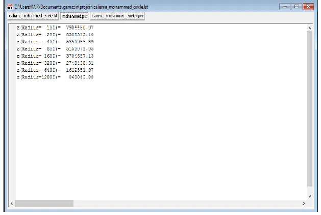
The relationship between the radius of the circular network overall and the lifetime of the WSN is a positive relationship. That is true and that it what we get as a result. We used 10 nodes with the initial energy (1 joule) and the distribution of these nodes in my experiment is random distribution (i.e., the distance among nodes not equal) in meter unit. Figure 4 shows the relationship between the radius and the WSN lifetime.

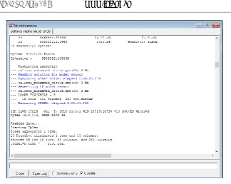
Figure 5 shows the number of iterations needed to reach the maximum lifetime of the designed WSN, also this figure shows the number of in-variable and out-variable of each node, in this paper we are focusing on the number of iterations to get optimal result. In the figure 4, when the radius is (200 m) then the maximum lifetime is (8588313.10 s). Figure 6 shows that the optimal solution (maximum lifetime) of the designed WSN by using LP is (8588313.103448 s) these result is accepted and expressed as an optimal solution.

4. CONCLUSION

Optimal planning of WSNs is a mind-boggling issue, because of the high level of adaptability of flexibility of this kind of network. Hence, it is attractive to have apparatuses that bolster this assignment. In addition, as arranging is normally in view of streamlined system models, the dependability of arranging apparatuses is essential. This paper has exhibited an advancement system to all the while augment lifetime and limit the normal number of bundle bounces for WSN systems. Moreover, we have likewise composed a calculation that accomplishes comes about tantamount to an advancement issue. In both cases, we have considered two sorts of hubs: hubs with enduring batteries, or essential hubs, and hubs with standard batteries, or optional hubs. The objective of the streamlining structure and the task calculation is to send essential hubs, with the goal that lifetime is boosted. The enhancement system comprises of two LP issues.

[image:4.595.55.280.272.377.2]

(5)

about. Reenactment comes about display a nearby similitude with those of the improvement, which proposes that the streamlined system demonstrate in the advancement structure is substantial.

We investigated the stream directing issue for WSN with the target of expanding system lifetime existing stream steering arrangements. For augmenting system lifetime, require information created at every hub and similarly beginning vitality esteem. We get optimal result by augmenting the lifetime of the system. Getting a high vitality when following from jump to bounce (from sensor hub to the following

sensor hub) coming to manager hub is a decent element and most imperative parameter when designing a wireless network.

The theoretical lifetime result while using LP for designing WSN is (8588313.10 s) when the radius is (200 m), we get an optimal result (practical lifetime result) equal to (8588313.103448 s). This result is perfect and we got maximum lifetime for proposed WSN in this paper, the goal is done.

Fig -4: Output result shows the relationship between the radius (in meters) and the network lifetime (in seconds).

[image:5.595.151.466.248.459.2] [image:5.595.152.464.490.737.2]

(6)

Fig -6: Status of the designed network.

REFERENCES

[1] Kim, B., & Park, H., & Kim, K., & Godfrey, D. Kim, K. (2017). A survey on Rael-Time Communications in Wireless Sensor Networks, Wireless Communications and Mobile Computing Journal, 1-14, doi: 10.1155/2017/1864847, 2017.

[2] Kiani, F., & Amiri, E., & Zamani, M., & Khodadadi, T., & Abdul Manaf, A. (2015). Efficient intelligent energy routing protocol in wireless sensor networks, International Journal of Distributed Sensor Networks, 2015, 1-13, doi: 10.1155/2015/618072.

[3] Kiani, F. (2014). Designing New Routing Algorithms Optimized for Wireless Sensor Network, LAP LAMBERT Academic Publishing, Dusseldorf, Germany.

[4] Santi, P. (2005). Toplogy Control in Wireless Ad-hoc and Sensor Networks, Wiley Online Library Books.

[5] Zhang, H., & Wang, H., & Feng H., & Liu B., & Gui B. (2009). A Heuristic Greedy Optimum Algorithm for Target Coverage in Wireless Sensor Networks, IEEE Computer Society, 9, pp. 39-42.

[6] Akshaye, D., & Sushil, K. (2008). A Distributed Algorithmic Framework for Coverage Problems in Wireless Sensor Networks, IEEE Parallel and Distributed Processing , pp. 1-8.

[7] Kumar, J., & Suman, S. (2014). State of Art Techniques for Wireless Sensor Network Lifetime Maximization, International Journal of Enhanced Research in Science Technology & Engineering, ISSN: 2319-7463 3 (1), pp: 275-279,

[8] Shi, L., & Zhang, J., & Shi, Y., & Ding, X., & Wei, Z. (2015). Optimal Base Station Placement for Wireless Sensor Networks with Successive Interference Cancellation, Sensors (Basel), 15(1), pp.1676-90.

[9] Singh, A., & Sharma, T. P. (2014). A survey on area coverage in wireless sensor networks, Control, Instrumentation, Communication and Computational Technologies (ICCICCT), International Conference, pp. 829-836.

[10] Anastasi, G., & Conti, M., & Di Francesco, M., & Passarella, A. (2009). Energy conservation in wireless sensor networks: a survey, Ad-Hoc Networks, 7 (3), 537-568,

[11] Rosenthal, R.E. (2007). GAMS- A User’s Guide, GAMS Development Corporation, Washington, DC, USA.

[12] Robichaud, V. (2010). An Introduction to GAMS, a pedagogical paper is an extract from “GAMS an

Introduction”.

http://anciensite.pep-net.org/fileadmin/medias/pdf/GAMSManual.pdf

[13] Ignacio, E. G. (1991). Introduction to GAMS, Department of Chemical Engineering, Carnegie Mellon University, Pittsburgh, PA 15213,

[image:6.595.148.473.54.312.2]

Maximizing Wireless Sensor Network Lifetime based on Linear Programming Method