Multi Threshold Algorithm Based on Havrda and Charvat Entropy for Edge Detection in Satellite Grayscale Images

(1)

http://dx.doi.org/10.4236/jsea.2014.71005

Multi-Threshold Algorithm Based on Havrda and Charvat

Entropy for Edge Detection in Satellite Grayscale Images

Mohamed A. El-Sayed1,2, Hamida A. M. Sennari3

1

Department of Mathematics, Faculty of Science, Fayoum University, Al Fayoum, Egypt; 2Assistant Professor of Computer Science, Taif University, Taif, KSA; 3Department of Mathematics, Faculty of Science, Aswan University, Aswan, Egypt.

Email: [email protected]

Received November 27th, 2013; revised December 25th, 2013; accepted January 2nd, 2014

Copyright © 2014 Mohamed A. El-Sayed, Hamida A. M. Sennari. This is an open access article distributed under the Creative Commons Attribution License, which permits unrestricted use, distribution, and reproduction in any medium, provided the original work is properly cited. In accordance of the Creative Commons Attribution License all Copyrights © 2014 are reserved for SCIRP and the owner of the intellectual property Mohamed A. El-Sayed, Hamida A. M. Sennari. All Copyright © 2014 are guarded by law and by SCIRP as a guardian.

ABSTRACT

Automatic edge detection of an image is considered a type of crucial information that can be extracted by apply- ing detectors with different techniques. It is a main tool in pattern recognition, image segmentation, and scene analysis. This paper introduces an edge-detection algorithm, which generates multi-threshold values. It is based on non-Shannon measures such as Havrda & Charvat’s entropy, which is commonly used in gray level image analysis in many types of images such as satellite grayscale images. The proposed edge detection performance is compared to the previous classic methods, such as Roberts, Prewitt, and Sobel methods. Numerical results underline the robustness of the presented approach and different applications are shown.

KEYWORDS

Multi-Threshold; Edge Detection; Measure Entropy; Havrda & Charvat’s Entropy

1. Introduction

Edge detection is a very important tool used in many applications of image processing to obtain information from the frames as a preparatory step to feature extraction and object segmentation. This phase detects outlines of an object and boundaries between objects and the background in the image [1]. The detection results benefit applications such as optical character recognition [2], infrared gait recognition [3,4], automatic target recognition [5], detection of video changes [6], and medical image applications [7].

Edge detection concerns localization of abrupt changes in the gray level of an image [8]. Edge detection can be defined as the boundary between two regions separated by two relatively distinct gray level properties [9]. The causes of the region dissimilarity may be due to some factors such as the geometry of the scene, the radio me- tric characteristics of the surface, the illumination and so on [10]. An effective edge detector reduces a large amount of data but still keeps most of the important feature of

the image. Edge detection refers to the process of locat- ing sharp discontinuities in an image [11,12].

Many operators have been introduced in the literature, for example, Roberts, Sobel and Prewitt [13-17]. Edges are mostly detected using either the first derivatives, called gradient, or the second derivatives, called Laplacien. Laplacien is more sensitive to noise since it uses more information because of the nature of the second derivatives.

(2)

decrease the computation time compared with Canny and LoG method. The results were very good compared with the well-known Roberts, Prewitt, and Sobel gradient results.

The outline of the paper is as follows. In Section 2, we have presented the classical edge detection methods that related to the paper. Image thresholding based on Havrda & Charvat’s entropy is presented in Section 3. Section 4 de- scribes the edge detection that was based on entropy. Sec- tion 5 illustrates the multi-threshold algorithm based on Havrda and Charvat entropy for edge detection. In Sec- tion 6, we have presented the effectiveness of proposed algorithm in the case of satellite grayscale images, and also we compared the results of the algorithm with sever- al leading edge detection methods such as Roberts, Pre- witt, and Sobel methods in the same section. Conclusions are presented in Section 7.

2. Classical Edge Detection Methods

Five most frequently used edge detection methods are used for comparison. These are: Gradient operators (Ro- berts, Prewitt, Sobel), Laplacian of Gaussian (LoG or Marr-Hildreth) and Gradient of Gaussian (Canny) edge detections [19,20]. People which would like to read about this subject are referred to [21-23] evaluation stu- dies of edge detection algorithms according to different criteria. The details of methods as follows,

2.1. Roberts Edge Detector

The Roberts Cross operator performs a simple, quick to compute, 2-D spatial gradient measurement on an image as shown in Figure 1. It thus highlights regions of high spatial frequency which often correspond to edges. In its most common usage, the input to the operator is a grayscale image, as is the output. Pixel values at each point in the output represent the estimated absolute magnitude of the spatial gradient of the input image at that point [20].

2.2. Prewitt Edge Detector

The Prewitt edge detector is an appropriate way to estimate the magnitude and orientation of an edge. Although differential gradient edge detection needs a rather time consuming calculation to estimate the orientation from the magnitudes in the x and y-directions, the compass edge detection obtains the orientation directly from the kernel with the maximum response. The Prewitt operator is limited to 8 possible orientations, however experience shows that most direct orientation estimates are not much more accurate. This gradient based edge detector is estimated in the 3 × 3 neighbourhood for eight directions as shown in Figure 2. All the eight convolution masks are calculated. One convolution mask is then selected, namely that with the largest module [20].

1 0 0 −1

0 −1 1 0

[image:2.595.335.507.94.226.2]

Gx Gy

Figure 1. Roberts gradient estimation operator.

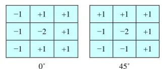
−1 +1 +1 +1 +1 +1

−1 −2 +1 −1 −2 +1 −1 +1 +1 −1 −1 +1

[image:2.595.341.504.157.226.2]

0˚ 45˚

Figure 2. Prewitt gradient estimation operator. 2.3. Sobel Edge Detector

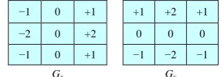
The operator consists of a pair of 3 × 3 convolution ker-nels as shown in Figure 3. One kernel is simply the other rotated by 90˚.

These kernels are designed to respond maximally to edges running vertically and horizontally relative to the pixel grid, one kernel for each of the two perpendicular orientations. The kernels can be applied separately to the input image, to produce separate measurements of the gradient component in each orientation (call these Gx and

Gy). These can then be combined together to find the ab-

solute magnitude of the gradient at each point and the orientation of that gradient [20]. The gradient magnitude is given by:

2 2

x y

G G G= +

Typically, an approximate magnitude is computed us-ing:

x y

G G G= +

which is much faster to compute.

The angle of orientation of the edge (relative to the pixel grid) giving rise to the spatial gradient is given by:

(

)

arctan Gy Gx θ =

2.4. Canny Edge Detector

(3)

−1 0 +1 +1 +2 +1 −2 0 +2 0 0 0 −1 0 +1 −1 −2 −1

[image:3.595.363.488.83.175.2]

Gx Gy

Figure 3. Sobel gradient estimation operator.

Step 1: The first step is to filter out any noise in the original image before trying to locate and detect any edges. It uses a filter based on a Gaussian (bell curve), where the raw image is convolved with a Gaussian filter. The result is a slightly blurred version of the original which is not affected by a single noisy pixel to any sig nificant degree. The Gaussian mask used in my imple-mentation is shown in Figure 4 with σ = 1.4.

Step 2: After smoothing the image and eliminating the noise, the next step is to find the edge strength by taking the gradient of the image using the Sobel operator uses a pair of 3 × 3 convolution masks. The approximate gra-dient magnitude is given by G G G= x + y .

Step 3: Finding the edge direction is trivial once the gradient in the x and y directions are known. However, you will generate an error whenever sumX is equal to zero. So in the code there has to be a restriction set whenever this takes place. Whenever the gradient in the x direction is equal to zero, the edge direction has to be equal to 90 degrees or 0 degrees, depending on what the value of the gradient in the y-direction is equal to. If Gy has a

value of zero, the edge direction will equal 0 degrees. Otherwise the edge direction will equal 90 degrees. The formula for finding the edge direction is just:

(

)

arctan Gy Gx θ =

Step 4: Once the edge direction is known, the next step is to relate the edge direction to a direction that can be traced in an image. So if the pixels of a 5 × 5 image are aligned as follows in Figure 5.

Then, it can be seen by looking at pixel “a”, there are only four possible directions when describing the sur- rounding pixels, 0 degrees (in the horizontal direction), 45 degrees (along the positive diagonal), 90 degrees (in the vertical direction), or 135 degrees (along the negative diagonal). So now the edge orientation has to be resolved into one of these four directions depending on which direction it is closest to (e.g. if the orientation angle is found to be 3 degrees, make it zero degrees). Think of this as taking a semicircle and dividing it into 5 regions as shown in Figure 6.

Therefore, any edge direction falling within the range (0 to 22.5 & 157.5 to 180 degrees) is set to 0 degrees. Any edge direction falling in the range (22.5 to 67.5 degrees) is set to 45 degrees. Any edge direction falling in the range (67.5 to 112.5 degrees) is set to 90 degrees. And finally, any edge direction falling within the range (112.5 to 157.5 degrees) is set to 135 degrees.

2 4 5 4 2

1

159

4 9 12 9 4

5 12 15 12 5

4 9 12 9 4

2 5 5 5 2

Figure 4. Discrete approximation to Gaussian function with σ = 1.4.

× × × × ×

× × a × × × × × × ×

[image:3.595.90.251.85.141.2]

× × × × ×

[image:3.595.313.501.90.386.2]

Figure 5. The pixel “a” and the possible directions.

Figure 6. The range of edge direction in the five regions.

Step 5: After the edge directions are known, nonmaximum suppression now has to be applied. Nonmaximum suppression is used to trace along the edge in the edge direction and suppress any pixel value (sets it equal to 0) that is not considered to be an edge. This will give a thin line in the output image.

Step 6: Finally, hysteresis is used as a means of elimi-nating streaking. Streaking is the breaking up of an edge contour caused by the operator output fluctuating above and below the threshold. If a single threshold, T1 is

ap-plied to an image, and an edge has an average strength equal to T1, then due to noise, there will be instances

where the edge dips below the threshold. Equally it will also extend above the threshold making an edge look like a dashed line. To avoid this, hysteresis uses 2 thresholds, a high and a low. Any pixel in the image that has a value greater than T1 is presumed to be an edge pixel, and is

marked as such immediately. Then, any pixels that are connected to this edge pixel and that have a value greater than T2 are also selected as edge pixels. If you think of

following an edge, you need a gradient of T2 to start but

you don’t stop till you hit a gradient below T1.

3. Havrda & Charvat’s Entropy

[image:3.595.379.471.327.384.2]

(4)

statistical moments of the gray level histogram of the image. The image histogram carries important informa-tion about the content of an image and can be used for discriminating the abnormal tissue from the local healthy background. Considering the gray level histogram

{

h i Ni, =0,1, 2,, g−1

}

where Ng is the number of dis-

tinct gray levels in the ROI (region of interest). If n is the total number of pixels in the region, then the normalized histogram of the ROI is the set

{

H i Ni, =0,1, 2,, g−1

}

,

where Hi=h ni . The source symbol probabilities is

{

i, 0,1, 2, , g 1

}

H= H i N=  ₋ . This set of probabilities must satisfy the condition, 0≤Hi≤1. The average information per source output, denoted S(H) [25], Shannon entropy may be described as:

( )

1

( )

0 log g N i i i

S H H H

−

=

= −

∑

(2) If we consider that a system can be decomposed in two statistical independent subsystems A and B, the Shannon entropy has the extensive property (additivity)

(

)

( )

S A+B =S A +S B , this formalism has been shown to be restricted to the Boltzmann-Gibbs-Shannon (BGS) statistics.

However, for non-extensive systems, some kind of ex- tension appears to become necessary. Havrda & Char- vat’s [26,27] has proposed a generalization of the BGS statistics which is useful for describing the thermo statistical properties of non-extensive systems. It is based on a generalized entropic form,

1 0 1 1 1 g N i i

HC_α Hα

α

−

=

 

= _ − _

− 

∑

 (3)

where the real number α is a entropic index that charac-terizes the degree of non-extensivity. This expression re- covers to BGS entropy in the limit α→1. Havrda & Charvat’s entropy has a non-extensive property for statis-tical independent systems, defined by the following rule [28]:

(

)

( )

( ) (

)

( )

1 .

HC A B HC A HC B HC A HC B

α α α

α α

α

+ = + + −

⋅ ⋅ (4)

Similarities between Boltzmann-Gibbs and Shannon entropy forms give a basis for possibility of generaliza-tion of the Shannon’s entropy to the Informageneraliza-tion Theory. This generalization can be extended to image processing areas, specifically for the image segmentation, applying Havrda & Charvat’s entropy to threshold images, which have non-additive information content.

Considering HC_α ≥0 in the pseudo-additive formal-ism of Equation (4), three different entropies can be de-fined with regard to different values of α .

For α<1, the Havrda & Charvat’s entropy becomes a “sub extensive entropy” where:

(

)

( )

HCα A+B <HCα A +HCα B (5)

For α =1, the Havrda & Charvat’s entropy reduces to an standard “extensive entropy” where:

(

)

( )

HCα A+B =HCα A +HCα B (6)

For α >1, the Havrda & Charvat’s entropy becomes a “super extensive entropy” where:

(

)

( )

HCα A+B >HCα A +HCα B (7)

Let f(x, y) be the gray value of the pixel located at the point (x, y). In a digital image

( )

{

}

{

}

{

f x y x, ∈ 1, 2,,M ,y∈ 1, 2,,N

}

of size M × N, let the histogram be h(a) for a∈

{

0,1, 2,, 255

}

with f as the amplitude (brightness) of the image at the real coor-dinate position (x, y). For the sake of convenience, we denote the set of all gray levels

{

0,1, 2,, 255

}

as G. Global threshold selection methods usually use the gray level histogram of the image. The optimal threshold t* is determined by optimizing a suitable criterion function obtained from the gray level distribution of the image and some other features of the image.

Let t be a threshold value and B = {b0, b1} be a pair of

binary gray levels with

{

b b₀, ₁

}

∈G. Typically b0 and b1

are taken to be 0 and 1, respectively. The result of thre-sholding an image function f(x, y) at gray level t is a bi-nary function f_t

(

x y,

)

such that f_t

(

x y,

)

=b₀ if

(

,

)

t

f x y ≤t otherwise, f_t

(

x y,

)

=b₁. In general, a thre-sholding method determines the value t* of t based on a certain criterion function. If t* is determined solely from the gray level of each pixel, the thresholding method is point dependent [25].

Let h h1, 2,,hk be the probability distribution for an

image with k gray-levels. From this distribution, we de-rive two probability distributions, one for the object (class A) and the other for the background (class B), giv-en by: 1 2 1 2 : , , , , : , , , t A

A A A

t t k B

B B B

h

h h

H H H

h h h

H H H

λ

λ + +

  (8) and where 1 1 , t k

A i B i i i t

H h H h

= = +

=

∑

=

∑

(9) The Havrda & Charvat’s entropy of order q for each distribution is defined as:

( )

1 1 1 1 1 1 and 1 1 t A i k B i t HC A HC B α α α α λ α λ α = = +   = _ − _ −     = _ − _ −  

∑

(10)

The Havrda & Charvat’s entropy HCα is parametri-

(5)

measure between the two classes (object and background). When HCα is maximized, the luminance level t

that maximizes the function is considered to be the opti-mum threshold value.

( )

( ) (

)

( )

* _Argmax ₁

. t G

t HC A HC B

HC A HC B

α α

∈

= _ + + −

⋅ ⋅ _ (11)

In the proposed scheme, first create a binary image by choosing a suitable threshold value using Havrda & Charvat’s entropy. The technique consists of treating each pixel of the original image and creating a new im-age, such that f_t

(

x y,

)

=0 if f x yt

( )

, ≤t*

( )

q otherwise,

(

,

)

1 t

f x y = for every x∈ 1 2

{

, ,,M

}

, y∈ 1 2

{

, ,,N

}

. When α→1, the threshold value in Equation (3), equals to the same value found by Shannon’s method. Thus this proposed method includes Shannon’s method as a special case. The following expression can be used as a criterion function to obtain the optimal threshold at

1 α→ .

(

)

( )

*

1 Argmax . t G

t α HC_α A HC_α B

∈

= = _ + _ (12)

The Havrda_Charvat_T procedure to select suitable threshold value t* with α for grayscale image f can now be described as follows:

Procedure Havrda_Charvat_T,

Input: An image f of size r × c, and α>0.

Output: optimal threshold t* of f. Begin

1. Let f(x, y) be the original gray value of the pixel at the point (x, y), x = 1.. r, y = 1.. c.

2. Calculate the probability distribution0 ≤ hi ≤ 255.

3. For all t∈{0, 1, …, 255},

i. Calculate HA, HB, λA, and λB using Equations

(8) and (9).

ii. Find optimum threshold value t*, such that

( )

( ) (

)

( )

* _Argmax ₁

. t G

t HC A HC B

HC A HC B

α α α α α α ∈ = _ + + − ⋅ ⋅ _ End.

The technique consists of treating each pixel of the original image and creating a new image, such that

(

,

)

0 t

f x y = if

( )

*

( )

,

t

f x y ≤t α otherwise, f_t

(

x y,

)

=1

for every x∈ 1 2

{

, ,,M

}

, y∈ 1 2

{

, ,,N

}

.

4. Detecting of the Edges

We will use the usual masks for detecting the edges [29]. A spatial filter mask may be defined as a matrix w of size

m × n. Assume that m = 2μ + 1 and n = 2ρ + 1, where μ, ρ are nonzero positive integers. For this purpose, smallest

meaningful size of the mask is 3 × 3. Such mask coefficients, showing coordinate arrangement as Figure 7(a). Image region under the above mask is shown as Figure 7(b).

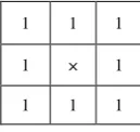
In order to edge detection, firstly classification of all pixels that satisfy the criterion of homogeneousness, and detection of all pixels on the borders between different homogeneous areas. In the proposed scheme, first create a binary image by choosing a suitable threshold value using Havrda & Charvat entropy. Window is applied on the binary image. Set all window coefficients equal to 1 ex-cept centre, centre equal to × as shown in Figure 8.

Move the window on the whole binary image and find the probability of each central pixel of image under the window. Then, the entropy of each central pixel of image under the window is calculated as S(CPix) = –pcln(pc).

Where, pc is the probability of central pixel CPix of bi-

nary image under the window. When the probability of central pixel, pc = 1, then the entropy of this pixel is zero.

Thus, if the gray level of all pixels under the window homogeneous, pc= 1 and S = 0. In this case, the central pi-

xel is not an edge pixel. Other possibilities of entropy of central pixel under window are shown in Table 1.

w(–1,−1) w(−1,0) w(−1,1) w(0,−1) w(0,0) w(0,1) w(1,−1) w(1,0) w(1,1)

(a)

f(x−1,y−1) f(x−1,y) f(x−1,y+1) f(x,y−1) f(x,y) f(x,y+1) f(x+1,y−1) f(x+1,y) f(x+1,y+1)

[image:5.595.352.495.371.529.2]

(b)

Figure 7. Coordinate arrangement and image region under 3 × 3 mask.

1 1 1

1 × 1

[image:5.595.390.455.571.632.2]

1 1 1

Figure 8. Window coefficients of 3 × 3 mask. Table 1. p and S of central under window.

p 1/9 2/9 3/9 4/9

S 0.2441 0.3342 0.3662 0.3604

p 5/9 6/9 7/9 8/9

[image:5.595.308.538.671.737.2]

(6)

In cases pc = 8/9, and pc = 7/9, the diversity for gray

level of pixels under the window is low. So, in these cas-es, central pixel is not an edge pixel. In remaining cascas-es,

pc≤ 6/9, the diversity for gray level of pixels under the

window is high. The complete algorithm can now be described as follows:

Algorithm HCEdgeDetection; Input: A grayscale image A (M × N).

Output: The edge detection image g.

Begin

1. Select suitable t*, α, using Havrda_Charvat_T pro-cedure.

2. Create a binary image:

If f(x, y) ≤ t* α) then f (x,y) = 0 Else f(x, y) = 1. 3. Create a mask w, with dimensions m × n: Normally, m = n = 3. μ = (m−1)/2 and ρ = (n−1)/2.

4. For all 1 ≤ x≤ M and 1 ≤ y ≤ N: Find g an output image by set g = f.

5. For all ρ + 1≤ y ≤ N−ρ and μ + 1 ≤ x ≤ M−μ, checking for edge pixels:

i. sum = 0;

ii. For all −ρ ≤ k ≤ ρ and −μ ≤ j ≤ μ: If (f(x, y) = f (x+j, y+k)) Then

Sum = sum + 1.

iii. If (sum > 6) Then g(x,y)=0 Else g(x,y) = 1.

End algorithm.

5. Proposed Algorithm

Here, the algorithm produces three different threshold values t1, t2 and t3. We use Havrda_Charvat_T procedure,

to find the threshold value t1 through the entire image.

Then we split the image by t1 into two grayscale parts,

the object and background. Applying the Equation (11), to find the locals threshold values t2 and t3 of object and

background, respectively. Independently, we apply HC EdgeDetection Procedure with threshold values t1, t2 and

t3. We merge the resultant edge images to obtain the re-

constructed edge image.

In order to minimize the execution time, we deal with the histogram vectors, 0, 1, ···, t1 and t1 + 1, ···, 255 of

object and background parts, respectively rather than the matrices size of them.

The steps of proposed algorithmare as follows: 1- Read the grayscale level image, I = imread (‘test. tif’);

2- Calculate the histogram H with 256 elements of I; 3- Call Havrda_Charvat_T(H, α) to find the optimal

threshold value, t1;

4- Divide H into two parts HLow and HHigh using t1.

5- Recall Havrda_Charvat_T(HLow, α) to find the

op-timal threshold value t2;

6- Recall Havrda_Charvat_T(HHigh, α) to find the

op-timal threshold value t3;

7- Now we have 3 values of the threshold, t2 < t1 < t3.

Reconstruct bitmap image f, such that: if (Ix,y < t1and Ix,y

>= t2) or (Ix,y >= t3) then fx,y=1; end;

8- Call the procedure HCEdgeDetection(f) to find edge image g.

9- Display the image g, imshow(g);

The above procedures can be done together in the fol-lowing MATLAB program:

I=imread(‘test.tif’); alpha=0.1;

[M,N,R]=size(I);

if R==3 I=rgb2gray(I); end; H = imhist(I);

[T1, Max1, Loc1] =

Havrda_Charvat_T(H,alpha); HLow= H (1:Loc1-1,:);

[T2, Max2, Loc2]=

Havrda_Charvat_T(HLow,alpha); HHigh= H (Loc1:size(H),:);

[T3, Max3, Loc3] =

Havrda_Charvat_T(HHigh,alpha); f=zeros(M,N);

for i=1:M; for j=1:N;

if ((I(i,j) >= T2)&(I(i,j) < T1)) |(I(i,j) >= T3) f(i,j)=1; end; end;

end

[g]= HCEdgeDetection(f); figure; imshow(g);

6. Results and Discussion

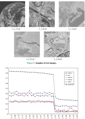
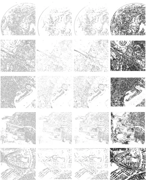
In order to test the method proposed in this paper and compare with the other edge detectors, common gray level test images with different resolutions and sizes are detected by Canny, LOG, Roberts, Prewitt, Sobel and the proposed method respectively. The performance of the proposed scheme is evaluated through the simulation results using MATLAB. Prior to the application of this algorithm, no pre-processing was done on the tested images (Figure 9).

The algorithm has two main phases global and local enhancement phase of the threshold values and detection phase, we present the results of implementation on these images separately. Here, we have used in addition to the original gray level function f(x, y), a function g(x, y) that is the average gray level value in a 3 × 3 neighborhood around the pixel (x, y). We use MATLAB to calculate the average time for each method at different images size by repeating 10 times for each type of image. As shown in

(7)

2_1_11.tif 2_1_02.tif 2_1_10.tif

[image:7.595.121.481.81.587.2]

2_2_07.tif 5_2_09.tif

Figure 9. Samples of test images.

Figure 10. Comparison of run time between some classical methods and proposed method on the same datasets.

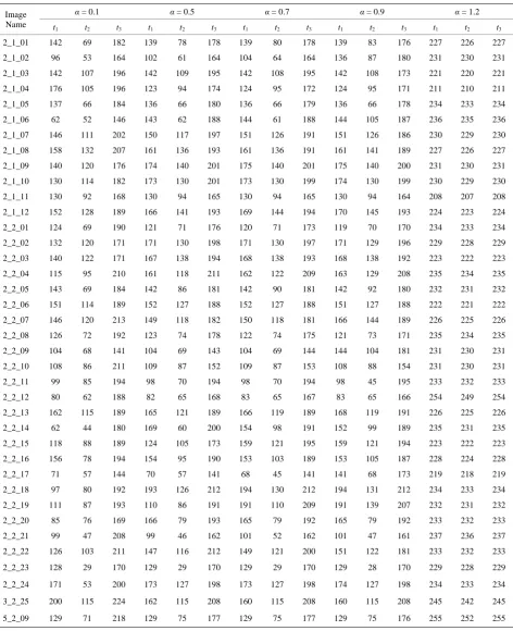
It has been observed that the proposed edge detector works effectively for different gray scale digital images as compare to the run time of classical methods. Some selected results of edge detections for these test images using the classical methods and proposed scheme are shown in

Figure 11 and Table 2.

10. Conclusion

This paper shows the new algorithm based on the Havrda

(8)

Figure 11. Edge detections of test images using the LoG method, Roberts method, Sobel method and proposed method, re-spectively.

execution time, and it is also considered as easy imple-mentation. The significance of this study lies in

[image:8.595.58.539.82.673.2]

(9)

[image:9.595.64.537.99.680.2]

Table 2. The threshold values of tested images with different values of α.

Image Name

α = 0.1 α = 0.5 α = 0.7 α = 0.9 α = 1.2

t1 t2 t3 t1 t2 t3 t1 t2 t3 t1 t2 t3 t1 t2 t3

2_1_01 142 69 182 139 78 178 139 80 178 139 83 176 227 226 227

2_1_02 96 53 164 102 61 164 104 64 164 136 87 180 231 230 231

2_1_03 142 107 196 142 109 195 142 108 195 142 108 173 221 220 221

2_1_04 176 105 196 123 94 174 124 95 172 124 95 171 211 210 211

2_1_05 137 66 184 136 66 180 136 66 179 136 66 178 234 233 234

2_1_06 62 52 146 143 62 188 144 61 188 144 105 187 236 235 236

2_1_07 146 111 202 150 117 197 151 126 191 151 126 186 230 229 230

2_1_08 158 132 207 161 136 193 161 136 191 161 141 189 227 226 227

2_1_09 140 120 176 174 140 201 175 140 201 175 140 200 231 230 231

2_1_10 130 114 182 173 130 201 173 130 199 174 130 199 230 229 230

2_1_11 130 92 168 130 94 165 130 94 165 130 94 164 208 207 208

2_1_12 152 128 189 166 141 193 169 144 194 170 145 193 224 223 224

2_2_01 124 69 190 121 71 176 120 71 173 119 70 170 234 233 234

2_2_02 132 120 171 171 130 198 171 130 197 171 129 196 229 228 229

2_2_03 140 122 171 167 138 194 168 138 193 168 138 192 223 222 223

2_2_04 115 95 210 161 118 211 162 122 209 163 129 208 235 234 235

2_2_05 143 69 184 142 86 181 142 90 181 142 92 180 232 231 232

2_2_06 151 114 189 152 127 188 152 127 188 151 127 188 222 221 222

2_2_07 146 120 213 149 118 182 150 118 181 166 144 189 226 225 226

2_2_08 126 72 192 123 74 178 122 74 175 121 73 171 235 234 235

2_2_09 104 68 141 104 69 143 104 69 144 144 104 181 231 230 231

2_2_10 108 86 211 109 87 152 109 87 153 108 88 154 231 230 231

2_2_11 99 85 194 98 70 194 98 70 194 98 45 195 233 232 233

2_2_12 80 62 188 82 65 168 83 65 167 83 65 166 254 249 254

2_2_13 162 115 189 165 121 189 166 119 189 168 119 191 226 225 226

2_2_14 62 44 180 169 60 200 154 98 191 152 99 189 235 231 235

2_2_15 118 88 189 124 105 173 159 121 195 159 121 194 223 222 223

2_2_16 156 78 194 154 95 190 153 103 189 153 105 187 228 224 228

2_2_17 71 57 144 70 57 141 68 45 141 141 68 173 219 218 219

2_2_18 97 80 192 193 126 212 194 130 212 194 131 212 234 233 234

2_2_19 111 87 193 110 86 191 191 110 209 191 139 207 232 231 232

2_2_20 85 76 169 166 79 193 165 79 192 165 79 192 233 232 233

2_2_21 99 47 208 99 46 162 101 52 162 101 47 161 237 236 237

2_2_22 126 103 211 147 116 212 149 121 200 151 122 181 233 232 233

2_2_23 128 29 170 129 29 170 129 29 170 129 28 170 229 228 229

2_2_24 171 53 200 173 127 198 173 127 198 174 127 198 234 233 234

3_2_25 200 115 224 162 115 208 160 115 208 160 115 208 245 242 245

5_2_09 129 71 218 129 75 177 129 75 177 129 75 176 255 252 255

that the traditional methods give rise to the exponential increment of computational time. Experiment results have demonstrated that the proposed scheme for edge detection can be used for different gray level digital images.

(10)

REFERENCES

[1] S. S. Alamri, N. V. Kalyankar and S. D. Khamitkar, “Image Segmentation By Using Edge Detection,” Inter- national Journal on Computer Science and Engineering

(IJCSE), Vol. 2, No. 3, 2010, pp. 804-807.

[2] J. Lzaro, J. L. Martn, J. Arias, A. Astarloa and C. Cuadra- do, “Neuro Semantic Thresholding Using OCR Software for High Precision OCR Applications,” Image Vision Com- puting, Vol. 28, No. 4, 2010, pp. 571-578.

http://dx.doi.org/10.1016/j.imavis.2009.09.011

[3] Z. Xue, D. Ming, W. Song, B. Wan and S. Jin, “Infrared Gait Recognition Based on Wavelet Transform and Sup- port Vector Machine,” Pattern Recognition, Vol. 43, No. 8, 2010, pp. 2904-2910.

http://dx.doi.org/10.1016/j.patcog.2010.03.011

[4] M. A. El-Sayed, “Edges Detection Based on Renyi Entro- py with Split/Merge,” Computer Engineering and Intelli- gent Systems (CEIS), Vol. 3, No. 9, 2012, pp. 32-41. [5] G. C. Anagnostopoulos, “SVM-Based Target Recognition

from Synthetic Aperture Radar Images Using Target Re- gion Outline Descriptors,” Nonlinear Analysis: Theory,

Methods & Applications, Vol. 71, No. 12, 2009, pp. e2934-e2939. http://dx.doi.org/10.1016/j.na.2009.07.030 [6] Y.-T. Hsiao, C.-L. Chuang, Y.-L. Lu and J.-A. Jiang,

“Robust Multiple Objects Tracking Using Image Seg- mentation and Trajectory Estimation Scheme in Video Frames,” Image Vision Computing, Vol. 24, No. 10, 2006, pp. 1123-1136.

http://dx.doi.org/10.1016/j.imavis.2006.04.002

[7] M. T. Doelken, H. Stefan, E. Pauli, A. Stadlbauer, T. Struf- fert, T. Engelhorn, G. Richter, O. Ganslandt, A. Doerfler and T. Hammen, “1H-MRS Profile in MRI Positive ver- sus MRI Negative Patients with Temporal Lobe Epilepsy,”

Seizure, Vol. 17, No. 6, 2008, pp. 490-497. http://dx.doi.org/10.1016/j.seizure.2008.01.008

[8] S. Kresic-Juric, D. Madej and S. Fadil, “Applications of Hidden Markov Models in Bar Code Decoding,” Interna- tional Journal of Pattern Recognition Letters, Vol. 27, No. 14, 2006, pp. 1665-1672.

[9] G. Markus, Essam A. EI-Kwae and R. K. Mansur, “Edge Detection in Medical Images Using a Genetic Algorithm,”

IEEE Transactions on Medical Imaging, Vol. 17, No. 3, 1998, pp. 469-474.

[10] M. Wang and Y. Shuyuan, “A Hybrid Genetic Algorithm Based Edge Detection Method for SAR Image,” IEEE Proceedings of the Radar Conference’05, 9-12 May 2005, pp. 1503-506.

[11] A. El-Zaart, “A Novel Method for Edge Detection Using 2 Dimensional Gamma Distribution,” Journal of Compu- ting Science, Vol. 6, No. 2, 2010, pp. 199-204.

[12] M. A. El-Sayed, “A New Algorithm Based Entropic Thre- shold for Edge Detection in Images,” International Jour-nal of Computer Science Issues (IJCSI), Vol. 8, No. 5, 2011, pp. 71-78.

[13] V. Aurich and J. Weule, “Nonlinear Gaussian Filters Per- forming Edge Preserving Diffusion,” Proceeding of the

17th Deutsche Arbeitsgemeinschaft für Mustererkennung

(DAGM) Symposium, Bielefeld, 13-15 September 1995,

Springer-Verlag, pp. 538-545.

[14] M. Basu, “A Gaussian Derivative Model for Edge Enhan- cement,” Pattern Recognition, Vol. 27, No. 11, 1994, pp. 1451-1461.

[15] G. Deng and L. W. Cahill, “An Adaptive Gaussian Filter for Noise Reduction and Edge Detection,” Proceeding of the IEEE Nuclear Science Symposium and Medical Ima- ging Conference, San Francisco, 31 October-6 November 1993, IEEE Xplore Press, pp. 1615-1619.

[16] C. Kang and W. Wang, “A Novel Edge Detection Method Based on the Maximizing Objective Function,” Pattern Recognition, Vol. 40, No. 2, 2007, pp. 609-618.

[17] Q. Zhu, “Efficient Evaluations of Edge Connectivity and Width Uniformity,” Image Vision Computing, Vol. 14, No. 1, 1996, pp. 21-34.

[18] B. Mitra, “Gaussian Based Edge Detection Methods—A Survey,” IEEE Transactions on Systems, Man and Cyber- netics, Vol. 32, No. 3, 2002, pp. 252-260.

[19] J. F. Canny, “A Computational Approach to Edge Detec- tion,” IEEE Transactions on Pattern Analysis and Ma-chine Intelligence (IEEE TPAMI), Vol. 8, No. 6, 1986, pp. 769-798.

[20] N. Senthilkumaran and R. Rajesh, “Edge Detection Tech- niques for Image Segmentation—A Survey,” Proceedings of the International Conference on Managing Next Gen- eration Software Applications (MNGSA-08), 2008, pp. 749-760.

[21] K. W. Bowyer, C. Kranenburg and S. Dougherty, “Edge Detector Evaluation Using Empirical ROC Curves,” IEEE Conference on Computer Vision and Pattern Recognition

(CVPR), 1999, pp. 354-359.

[22] M. Heath, S. Sarkar, T. Sanocki and K. W. Bowyer, “A Robust Visual Method for Assessing the Relative Perfor- mance of Edge Detection Algorithms,” IEEE Transac- tions on Pattern Analysis and Machine Intelligence (TPAMI), Vol. 19, No. 12, 1997, pp. 1338-1359.

http://dx.doi.org/10.1109/34.643893

[23] M. Shin, D. Goldgof and K. W. Bowyer, “An Objective Comparison Methodology of Edge Detection Algorithms for Structure from Motion Task,” IEEE Conference on Computer Vision and Pattern Recognition (CVPR), 1998, pp. 190-195.

[24] R. Deriche, “Using Canny’s Criteria to Derive a Recur- sively Implemented Optimal Edge Detector,” Internatio- nal Journal of Computer Vision (IJCV), Vol. 1, No. 2, 1987, pp. 167-187.

http://dx.doi.org/10.1007/BF00123164

[25] C. E. Shannon, “A Mathematical Theory of Communica- tion,” Bell System Technical Journal, Vol. 27, No. 3, 1948, pp. 379-423.

http://dx.doi.org/10.1002/j.1538-7305.1948.tb01338.x [26] A. P. S. Pharwaha and B. Singh, “Shannon and Non-

Shannon Measures of Entropy for Statistical Texture Fea- ture Extraction in Digitized Mammograms,” Proceedings of the World Congress on Engineering and Computer Sci- ence (WCECS), San Francisco, Vol. II, 20-22 October 2009.

(11)

Statistics,” Journal of Statistical Physics, Vol. 52, No. 1-2, 1988, pp. 479-487.

http://dx.doi.org/10.1007/BF01016429

[28] M. P. de Albuquerque, I. A. Esquef and A. R. Gesualdi Mello, “Image Thresholding Using Tsallis Entropy,” Pat- tern Recognition Letters, Vol. 25, No. 9, 2004, pp. 1059-

1065.

http://dx.doi.org/10.1016/j.patrec.2004.03.003