Model Reference based Tuning of PID Controller using
Bode's Ideal Transfer Function and Constrained Particle
Swarm Optimization
Anindya Bhattacharyya
RTSD,ICG,IGCAR Kalpakkam,Tamil Nadu
India
N.Murali
RTSD,ICG,IGCAR Kalpakkam, Tamil Nadu
India
ABSTRACT
A new method for designing PID Controllers using Bode’s ideal transfer function and constrained Particle Swarm Optimization (PSO) is proposed in this paper. Bode’s ideal transfer function is introduced using fractional calculus and Carlsson’s approximation is used for converting the transfer function from fractional to integer domain. The PID controller is designed by minimizing a hybrid objective function using PSO. Simulation examples confirming the effectiveness of the resulting controller are also discussed in detail and a performance comparison, highlighting the enhanced capability of PSO over other conventional mathematical optimization approaches, is also made in the paper.
General Terms
Self tuning PID controller, Particle Swarm Optimization
Keywords
PID, Bode’s ideal transfer function, PSO, Active Set optimization, Fractional Order Controllers
1.
INTRODUCTION
The last decade has seen a revival of interest in the field of fractional calculus and its applications [1-4]. Even though the application of the field in the areas of control engineering remains largely unexplored, preliminary results can be found in [1,9].
In the industrial arena more than 90 % of all controller used are PID as reported in [5]. Designing of PID controllers involves a search for four parameters so that the desired response and performance is obtained. As per standard notations used in the literature they are called proportional gain (Kp), Integral gain (Ki), Derivative gain (Kd) and derivative filter time constant (N).In search of more flexibility and better performance a number of different forms of PID control algorithms has been designed and implemented [5-7]. Of which notable variants are the two degree freedom PID controller by Araki et all [8] resulting in a six parameter tuning problem and the Fractional order PID controller [9] resulting in five parameter tuning problem. In this paper when we talk about PID controllers, the algorithm being referred to is the standard parallel non interacting form of PID better
The reason for ongoing research in the field of PID controller is that there is no one absolute method to tune the controller. In the last five decades a large number of analytical, experimental and computational methods has been published in peer reviewed literature but none of them are as simple and popular as the Ziegler-Nichols[10] method of tuning. A very good account of the published tuning methodologies can be found in O’Dwyer [7].The reason for so many types of tuning methodologies stem from the fact that the tuning methodology derived for a particular form of process is unable to achieve the required level of performance in a different process. In this paper we propose to design a process independent PID controller with the purpose of minimizing an objective function described later in section 4. The adopted strategy is known as model reference tuning where the open loop transfer function and hence the loop response is modified using the four tuning parameters Kp, Ki, Kd ,N so as to match the performance of the model reference transfer function[11]. The model reference transfer function used is the Bode’s ideal transfer function which is introduced using the concepts of fractional calculus[12]. The optimization problem is solved using Particle Swarm Optimization[13] with an adaptive inertial weight[14] .The advantage of this method lies in the fact that we have direct control on the time domain specifications of the controlled system unlike other optimization based PID tuning solution. This fact is suitably explained with the help of detailed case studies in section V. The paper is organized as follows. Section 2 reviews Bode‘s ideal transfer function, its characteristics and its integer order approximation. Section 3 introduces PSO and the variant used in this paper. Section 4 deals with control design and the objective function. Section 5 presents the simulation case studies followed by discussions and acknowledgements.
2. BACKGROUND THEORY ON BODE’S
IDEAL TRANSFER FUNCTION AND
MODEL REFERENCE TUNING
2.1 Fractional Differeintegrations
The integral-differential operator, denoted by
D
t is a notation for taking both fractional derivative and fractional integral in a single expression. When α > 0 it is called fractional derivative and when α < 0 it is called fractional integral. The unified integral-differential operator is shown in equation (1)
) 1 ....( 0 1 1 0 0 0
t t where dt where where dt d D
There are several different definitions of fractional derivatives and integral [3]. One of the most common definitions, the Caputo definition is given below in Eq (2)
)
2
....(
)
(
)
(
)
(
)
(
1
)
(
0 1 ) ( 0
N
m
dt
t
f
d
m
d
t
f
m
t
f
D
m m t m m i
The Laplace transformation of the Caputo derivative with initial conditions set to zero is given by equation (3):
)
3
(
...
)
(
)}
(
*
{
0D
f
t
s
F
s
R
L
t
2.2 Carlsson’s Approach to Integer order
Approximations
of
Fractional
Order
Elements
Carlsson and Halijack [15][16] proposed a simple method to find the integer order approximations of fractional order elements. The proposed approach used Newton’s approximation to find arbitrary
th (0≤
≤1) root of polynomial. According to Carlsson’s approach the first order approximations to Fractional Order (FO) integrator is given by Eq (4))
4
.(
...
1
*
s
m
p
m
p
m
p
m
p
s
s
p and m are integers such that
m
p
If we writem
p
m
p
then Eq.(4) can be rewritten as
) 5 .( ... 1 * s s s
Where1
1
and β > 1.For Fractional Order Differentiation similarly
Where
1
*
s
s
s
and1
1
and β < 1 …(6)Thus Right Hand Side (RHS) of Eq (5,6)
1
*
s
s
gives acommon first order approximate transfer function of FO differintegrals and the knowledge of the parameter β ( <1 or >1) is sufficient to transfer a fractional order transfer function to integer domain.
2.3 Bode’s Ideal Transfer Function and Its
Properties
Bode proposed that the ideal shape of the Nyquist plot for the open loop frequency response is a straight line in the complex plane, which provides theoretically infinite gain margin. Ideal open-loop transfer function is given by:
) 7 ...( ... ) ( R s s
L gcf
If < 0 then a fractional order derivative is formed while if > 0 a fractional order integral is formed. The constant is the slope of the magnitude curve of L(s) on a log-log scale and can take any real number as its value. The effect of is shown in Fig.1 where step response of closed loop Bode’s transfer function to varying (1 < <2) is shown.
Fig1: Effect of (1<<2) on closed loop system having integer approximated Bode’s ideal transfer function
From the figure it is clear that all other variables remaining constant the maximum peak overshoot Mp is solely a function
Fig.2a Bode plot showing the effect of varying (1<<2) on open loop system having integer approximated Bode’s ideal transfer function
The amplitude curve is a straight line of constant slope −20γ dB/dec ( the deviation in the figure is due to the integer order approximations), and the phase curve is a horizontal line at −γπ/2 rad.
Fig.2b Nyquist Plot showing the effect of varying (1<<2) on open loop system having integer approximated Bode’s ideal transfer function
The Nyquist curve consists, simply, on a straight line through the origin with arg L(jω) = −γπ/2 rad. gcf is the desired gain
crossover frequency which determines the bandwidth and speed of the system. At gcf the magnitude of L(s) is unity.
The major benefit achieved through this structure is iso-damping[1], i.e. overshoot being independent of the payload or the system gain.
2.4 Time Domain Characteristics
From[11, 17] we obtain the following expressions to construct Bode’s ideal transfer function i.e from the time domain specification using the following expressions we can determine the value of gcf and .
Mp= 0.8*(-1)*( -.75) Where 1 < < 2………..(8)
)
9
....(
...
)
724
.
(
*
)
157
.
1
(
*
131
.
2
gcf r
T
gcf s
T
/
)
*
cos(
4
(2% tolerance and 1.39 < < 2.0).…..(10)
Where Mp is the maximum peak overshoot ,Tr is the rise time and Ts the settling time.
Example: For a family of FOPTD it is required to design a control system such that Mp=5% and Ts=5 seconds. Using this specification we can derive the required parameters in Bode’s transfer function. Substituting Mp=.05 in Eq.(8) we get a quadratic equation with 2 real roots. The root lying between 1 and 2 is chosen for obvious reasons which gives us
=1.13.Substituting Ts=5 sec we get gcf =.9 rad/sec which
gives us an open loop transfer function
13 . 1
)
9
.
0
(
)
(
s
s
L
………...(11)The corresponding closed loop transfer function is
12 . 1
* 12 . 1 1
1 )
(
s s
TF ……….(12)
Carlssons approximation is used to convert the fractional order transfer function to integer order. First order Carlssons approximation gives us the following transfer function which serves as the reference model for PID tuning methodology presented in this paper.
1 * 632 . 1 * 12 . 1
1 * 77 . 0 )
( 2
s s
s s
TI ……..….(13)
For First Order Processes with Dead Time (FOPDT) the reference model is given by
)
(
*
)
(
)
(
LsI ID
s
T
s
e
T
………...(14)Fig.3 The performance of the model reference function after getting integer approximated for various dead times
(L).
3. PARTICLE SWARM OPTIMIZATION
Particle Swarm Optimization (PSO) was proposed by Kennedy and Eberhart[13] in 1995 based on the Swarm behavior exhibited by birds flocking or fishes schooling in nature. A good account of PSO and its variants are given in [18]. The algorithm is a metaheuristic methodology used for solving optimization problems.The PSO as it was originally conceived in [13] was unstable and had a tendency not to converge as oscillations ensued and became wider and wider, unless some damping was applied. The two most notable methods which solved this problem are Eberhart and Shi’s PSO with Inertia [14] and Clerc’s [27] PSO with Constriction. Here in this work we have used Eberhart and Shi’s PSO with inertia [14] which acts as a virtual mass to stabilize the motion of the particle. The inertia, a constant ranging between .5 to .9 and was scaled down from .9 to .5 linearly as the iteration progressed. during the simulations. A non zero inertial weight introduces a preference for the particle to move in the same direction it was going on the previous iteration. Decreasing the inertia over time makes the agents searching for the minima more flexible and searching more exploitative. Given below is the pseudocode form of the PSO algorithm used in simulation :Begin
Initialize the parameters: number of particles (n),
number of iterations allowed (bird_setp), the dimension of the search space (dim), initial inertia (wstart),
final inertia (wend). Current inertia (w),
C1= PSO constant signifying self confidence. C2= PSO constant signifying Swarm confidence. Current iteration number(iter),
R1=random(dim,n) R2=random(dim,n)
Start Iteration
while( iter<bird_setp ) iter = iter + 1;
w=((bird_setp - iter)*(wstart - wend))/(bird_setp) +wend; for i = 1 to n,
Evaluate fitness function for all the particles and store it in a variable named current_fitness(i).
End
for i = 1 : n
ifcurrent_fitness(i) <local_best_fitness(i) local_best_fitness(i) = current_fitness(i); local_best_position(:,i) = current_position(:,i) end
end
[current_global_best_fitness,g] = min(local_best_fitness) ifcurrent_global_best_fitness<global_best_fitness global_best_fitness = current_global_best_fitness; for i=1:n
globl_best_position(:,i) = local_best_position(:,g); end
end
velocity = w *velocity + c1*(R1.*(local_best_position-current_position)) + c2* (R2. * (globl_best_position-current_position));
current_position = current_position + velocity; end
End
The algorithm presented above is an unconstrained version of the PSO. For better performance it is necessary to constrain the solution space. Various methods has been proposed to solve constrained PSO [20-22].The method used in this work is direct implementation. The simplest direct implementation is to check for all the new particle locations to see whether all the constraints are met. The new locations are discarded if all the constraints are not met and new locations are replaced by newly generated location until all the constraints are met. Then the new solutions are evaluated using the standard PSO procedure.
4
.
MATHEMATICAL OPTIMIZATION
AND CONTROL DESIGN
Maximize/minimize:
f(x) ,where x= (x1,x2, x3 …xn) T
x
ε
Rn……..…….(15)Subject to j(x) = 0, (j=1,2,3……M)
k(x) > 0 (k=1,2,3……N)
Where f(x) is the objective function being minimized and
j(x), k(x) are constraint equality and inequality
respectively. The components of x (x1, x2, x3 ……..xn) are
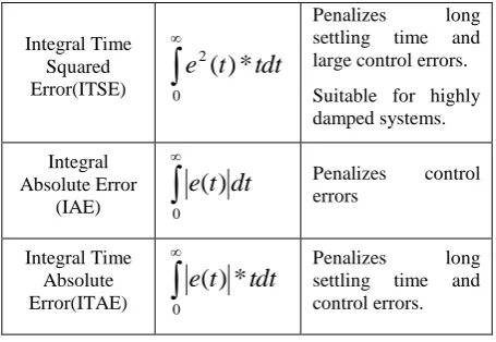
called the design variables and the vector x is often called the decision vector which varies in a n dimensional search space Rn. The space spanned by the decision variables is called the search space and the space formed by the objective is called the solution space. The optimization problem basically maps the search space Rn into the solution space R. Traditionally for PID optimization the objective functions used are given in Table 1 [24] along with their properties:
We propose to use a weighted combination of ISE and ITAE. The chosen objective function therefore is
dt t e t W dt t e W x
f
0 0 2 2
1* ( ) * ( )
)
(
where W1+W2=1……(16)
and e(t) is the difference between output of the model reference Bode’s Ideal Transfer function and the plant output. The transfer function for PID used is given by the Eq (17)
...(17)
1 * * * 1 1 ) ( ) ( s N T s T s T K s E s U d d i p
Where Ki=Kp/Ti and Kd=Kp*Td are integral action and the derivative action respectively. PID equation has 4 unknowns Kp ,Ki ,Kd and N so the search space has 4 dimensions. This four dimensional space is searched by the PSO algorithm in a manner that minimizes the objective function. Putting the control problem down formally
Minimize :
dt t e t W dt t e W x
f
0 0 2 2
1* () * ()
)
(
where x=(Kp,Ki,Kd,N)
R4 and W1+W2=1Subject to the condition 0< (Kp, Ki, Kd ,N) <100
[image:5.595.315.543.71.228.2]This optimization problem is solved by constrained PSO and the results are compared with that obtained by active set algorithm [25] and Ziegler-Nichols Method for a family of First Order Processes with Dead Time (FOPDT).
Table:1 Summary of objective functions
Performance
Index Equation Properties
Integral Squared Error
(ISE)
0 2
)
(
t
dt
e
Penalizes large control errors. Settling time longer than ITSE.
Suitable for highly
Integral Time Squared Error(ITSE)
0 2
*
)
(
t
tdt
e
Penalizes long settling time and large control errors. Suitable for highly damped systems.
Integral Absolute Error
(IAE)
0
)
(
t
dt
e
Penalizes errors controlIntegral Time Absolute Error(ITAE)
0
*
)
(
t
tdt
e
Penalizes settling time long and control errors.5. CASE STUDIES AND OBSERVATION
In this section we take a family of FOPDT and evaluate the effectiveness of the proposed methods against methods like Ziegler-Nichols, PSO without the Bode’s Ideal Transfer Function and Active-set algorithm [25]. The processes used in simulation purpose are taken from[26].L stands for the dead time andτ
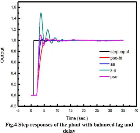
the time constant of the process.5.1 FOPTD Plant with A Balanced Lag And
Delay (L
τ)
A balanced lag and delay process is chosen as
1 5 . 1 5 ) ( s e s G s
p where lag L is 1 second and the time constant
τ is
1.5 second. The results of the tuning procedure are given in Table:2 and Fig:4Table2: Tuning results for a plant with balanced lag and delay
PSO & Bode’ s Ideal Transfer Function
PSO Active-set Ziegler -Nichols
Kp .14 .3381 .2440 .375
Ki .09 .1203 .1104 .22
Kd 1.8525 .1500 .0686 .16
N .0023 70.3118 10 10
Fig.4 Step responses of the plant with balanced lag and delay
5.2 Delay Dominated FOPTD Plant(L >>τ )
A delay dominated plant is chosen with transferfunction
1
05
.
)
(
s
e
s
G
s
p where lag L is .05 second
and the time constant
τ is
0.05 second. The simulation results are shown in Table 3 and Fig.5Table3: Tuning results for a plant with dominant delay
PSO & Bode’ s Ideal Transfer Function
PSO Active-set
Ziegler -Nichols
Kp .0561 .2026 .2067 .54
Ki .5168 .5876 .5874 .64
Kd .2838 .1.7854 .1554 .11
N .0014 .0029 .01 10
[image:6.595.53.283.75.293.2]
For a delay dominated plant the Active Set algorithm and PSO outperforms the proposed methodology. The Active Set algorithm outperforms the proposed methodology only because the initial values supplied to the function are very close to the actual values thereby reducing the nature of search from global to local. It is also observed that though the proposed methodology is outperformed it is still within the performance specifications
Fig.5 Step responses of the plant with a dominant delay
5.3 Lag Dominated FOPTD Plant(L << τ )
A lag dominated plant is chosen with transfer function1 11 . 1 ) (
105 .
s e s G
s
p . where lag L is0 .105 second and the time constant
τ is
1.11 second. The simulation results are shown in Table 4 and Fig.6Table 4: Tuning results for a plant with dominant lag
PSO & Bode’ s Ideal Transfer
Function
PSO Active-set Ziegler -Nichols
Kp .43 2.1907 3.17 1.75
Ki .64 .6389 .67 1
Kd .0 .5219 .4784 .38
N .64 7.42 11.1158 10
Fig.6 Step responses of the plant with a dominant lag [image:6.595.310.548.400.678.2]
6. CONCLUSION
In this paper we have explored the potentialities of Bode’s Ideal Transfer function in the field of PID controller tuning using Particle Swarm Optimization .A new methodology is proposed and simulation results validating the proposed methodology was presented. The proposed methodology performed satisfactorily when compared to other standard techniques.
8. REFERENCES
[1] D. Shantanu., "Functional fractional calculus for system identification & controls. ," Springer, 2008.
[2] J. Sabatier, O. P. Agrawal, and J. A. T. Machado, ADVANCES IN FRACTIONAL CALCULUS :Theoretical Developments and Applicationsin Physics and Engineering: Springer, 2007.
[3] I. Podlubny, Fractional Differential Equations: : An Introduction to Fractional Derivatives, Fractional Differential Equations, to Methods of Their Solution and Some of Their Applications, New York: Academic Press.1998
[4] K. B. Oldham, and J.Spanier, The Fractional Calculus: Theory and Application of Differentiation and Integration to Arbitrary Order, Academic Press New York 1974.
[5] K. J. Astrom, and T. Hagglund, “PID controller: Theory, design, and tuning.,” Instrument Society of America, 1995.
[6] A. Visioli, Practical PID Control: Springer-Verlag London Limited 2006.
[7] A. O'Dwyer, Handbook of PI and PID Controller Tuning Rules: Imperial College Press, 2006 2nd edition. [8] M. Araki et. all “Two Degree of Freedom PID
Controller” ” System,Control and Information, Vol 42, pp. pp 18-25, 1988.
[9] I.Petras, R. Caponetto, G. Dongola et al., FRACTIONAL ORDER SYSTEMS:Modeling and Control Applications: World Scientific, 2010.
[10]J. G. Ziegler, N. B. Nichols, and “ “Optimum settings for automatic controllers”,” in Trans. ASME, 1942, pp. 433-444.
[11]R. S. Barbosa, J. A. T. Machado, and I. M. Ferreira, “Tuning of PID Controllers Based on Bode’s Ideal Transfer Function,” Nonlinear Dynamic"s, Vol. 38, pp. 305–321, 2004.
[12][H. S. Farhad Farokhi, "A Robust Control-Design Method Using Bode’s Ideal Transfer Function."
[13]J. Kennedy & R. Eberhart, “Particle Swarm Optimization,” 1995.
[14]R. C. Eberhart, and Y. Shi, ““Comparing Inertia Weights and Constriction Factors in Particle Swarm Optimization”,” in Proceedings of the Congress on Evolutionary Computation 2000, pp. 84-88.
[15]G. E. Carlson, and C. A. Halijak, ““Simulation of the fractional derivative operator √s and the fractional integral operator 1/√s”,” in Central States Simulation Council Meeting on extrapolation of analog computation methods, Kansas State University, July 1961, pp. 1-22. [16]B. M. Vinagre, I. Podlubny, A. Hernandez et al., "Some
Approximations Of Fractional Order Operators Used In Control Theory And Applications." pp. 231–248. [17]S.Manabe, "The Non-Integer Integral and its application
to Control Systems." pp. 83-87.
[18]Y.S.Bijaya Ketan Panigrahi & Meng-Hiot Lim “Handbook of Swarm Intelligence Concepts, Principles and Applications,” Springer, 2011.
[19]M. Clerc et all. “The Swarm And The Queen: Towards A Deterministic And Adaptive Particle Swarm Optimization” in Proceedings of the Conference on Evolutionary Computation, 1999, pp. 1951-1957. [20]X. Hui & R. Eberhart, “Solving Constrained Nonlinear
Optimization Problem with Particle Swarm Optimization.”
[21]C. S. Thenehalli, “Design Optimization Using Augmented Lagrangian Particle Swarm Optimization,” Faculty of the Graduate School, The University of Texas at Arlington.
[22]K. E. Parsopoulos & M. N. Vrahatis, “Particle Swarm Optimization Method for Constrained Optimization Problems”.
[23]X. S. Yang, Introduction to Mathematical Optimization From Linear Programming to Metaheurestics: Cambridge International Science Publishing, 2009. [24]N. Pillay, “A Particle Swarm Optimization Approach for
Tuning Of SISO PID Control Loops” Masters, Department Of Electronic Engineering, Durban University of Technology, 2008.
[25]"MATLAB optimization toolbox user's guide ,The Mathworks Inc" The Mathworks Inc.
[26]S. Saha, S. Das, R. Ghosh et al., “Fractional order phase shaper design with Bode's integral for iso-damped control system,” ISA Transactions, vol. 49, pp. 196-206, 2012.