PARIS RESEARCH LABORATORY
d i g i t a l
October 1993 Jacques Garrigue
Hassan A¨ıt-Kaci
The Typed
Polymorphic
The Typed
Polymorphic
Label-Selective
-Calculus
Jacques Garrigue Hassan A¨ıt-Kaci
A reprint of this report will appear in the Proceedings of the 21st ACM Symposium on Principles of Programming Languages, (Portland, OR, January 1994), ACM Press.
Contact addresses of authors:
Jacques Garrigue
The University of Tokyo
Department of Information Science 7-3-1 Hongo, Bunkyo-ku
Tokyo 113, Japan
Hassan A¨ıt-Kaci [email protected]
Digital Equipment Corporation Paris Research Laboratory 85 Avenue Victor Hugo
92500 Rueil-Malmaison, France
c
Digital Equipment Corporation and University of Tokyo 1993
Formal calculi of record structures have recently been a focus of active research. However, scarcely anyone has studied formally the dual notion—i.e., argument-passing to functions by keywords, and its harmonization with currying. We have. Recently, we introduced the label-selective-calculus, a conservative extension of-calculus that uses a labeling of abstractions and applications to perform unordered currying. In other words, it enables some form of commutation between arguments. This improves program legibility, thanks to the presence of labels, and efficiency, thanks to argument commuting. In this paper, we propose a simply typed version of the calculus, then extend it to one with ML-like polymorphic types. For the latter calculus, we establish the existence of principal types and we give an algorithm to compute them. Thanks to the fact that label-selective-calculus is a conservative extension of-calculus by adding numeric labels to stand for argument positions, its polymorphic typing provides us with a keyword argument-passing extension of ML obviating the need of records. In this context, conventional ML syntax can be seen as a restriction of the more general keyword-oriented syntax limited to using only implicit positions instead of keywords.
R ´esum ´e
Functional programming, -calculus, types, polymorphism, record calculi, type inference, unification, concurrency
Acknowledgements
2 Motivation 3 2.1 Keywords: an enhancement for clarity : : : : : : : : : : : : : : : : : : 3 2.2 Relative positions versus combinators : : : : : : : : : : : : : : : : : : 4 2.3 A generic commutation capability : : : : : : : : : : : : : : : : : : : : 5
3 -Calculus with multiple channels 6
4 -Calculus with relative positions 7
5 The selective-calculus 8
6 Simple types 10
6.1 Syntax and types : : : : : : : : : : : : : : : : : : : : : : : : : : : : : 10 6.2 Record concatenation : : : : : : : : : : : : : : : : : : : : : : : : : : : 10 6.3 Record matching : : : : : : : : : : : : : : : : : : : : : : : : : : : : : : 12 6.4 Typing rules : : : : : : : : : : : : : : : : : : : : : : : : : : : : : : : : 13
7 Polymorphic selective-calculus 13
7.1 Syntax and types : : : : : : : : : : : : : : : : : : : : : : : : : : : : : 14 7.2 Type substitution : : : : : : : : : : : : : : : : : : : : : : : : : : : : : : 14 7.3 Typing rules : : : : : : : : : : : : : : : : : : : : : : : : : : : : : : : : 15 7.4 Type unification : : : : : : : : : : : : : : : : : : : : : : : : : : : : : : 15 7.5 Type inference : : : : : : : : : : : : : : : : : : : : : : : : : : : : : : : 16
They were both very pleased with this new view of the matter, which did credit to them both, and we all parted on the most friendly terms.
ROBERTGRAVES, I, Claudius
1 Introduction
The use of symbolic labels in programming languages is not new. This has been done in two ways. The first one, common to nearly all languages, is as field designators in record structures. Relatively recently, formalisms for records have been proposed. This started with Cardelli [6], was later extended to a second order calculus [7], and was followed by a number of record-type inference systems compatible with ML-style polymorphic type inference [22, 20, 13, 19]. Even more recently, a compilation method was proposed by Ohori [18], for an extension of-calculus containing polymorphically typed records.
Another way to use labels in programming languages has been as keywords for parameter-passing in procedure or function calls. This is the case in Common LISP [21], ADA [15], and LIFE [4]. However, in Common LISP or ADA, currying is not supported, which makes the situation rather mild. Although currying is supported in LIFE, even with keywords given in a different order, it is restricted nonetheless and does not accommodate implicit positions as it should. Indeed, fully flexible currying with the presence of keywords as well as explicit and implicit positions was until recently a still unexplored issue. Some proposals do offer this convenience of parameter-passing without modifying the core calculus [14, 17]. However, these are based on using a notion of store; that is, bindings from names to values. This introduces another parameterizing system, independent from -calculus. Even so, to our knowledge, no typing system has been proposed for them.
Our own proposal, as originally reported in [2], is to support this new convenience of labeling arguments directly in-calculus and accommodate selective unordered currying through commutation of arguments. In our view, the role of arguments is determined by their labels, which interact with their order.
Selective-calculus introduces two types of commutations. The first, and most immediate, is between symbolic labels. By analogy with tuples, when currying an expression f(p) a;q)b;. . .)we obtain an expression((f(p)a))(q)b))(. . .). But since there is no reason to apply f in this specific order, using the freedom provided by labels allows to curry in a different order; e.g., ((f(q)b))(p)a))(. . .). Suppressing superfluous parentheses, and limiting our consideration to two arguments, we obtain that the following equality must hold in our calculus:
f(p)a)(q)b)=f(q)b)(p)a):
However, this is true under a restriction: p and q must be distinct labels. Successive applications on the same label must not commute. Indeed, if the labels are equal, the order of these applications must be obeyed to be unambiguous.
ML-like language, together with inferred types.1
#let cons car=>a cdr=>b = a::b;;
cons : {car=>’a,cdr=>’a list} -> ’a list
#cons cdr=>[1];;
it : {car=>int} -> int list
The second commutation equality comes from a reversion of the analogy with tuples. That is, we can see a tuple as a record labeled with numbers: (a;b;. . .)=(1)a;2)b;. . .). If we applied the equality used for symbolic labels, we would obtain f(1)a)(2)b) = f(2)b)(1)a). But, since it is better to see unary application as implicitly using the label 1 and keep conventional currying, we would rather write f(1)a)(1)b), or simply, f a b as usual. To make this possible, we must define commutation differently on numbers: namely, f(2)b)(1)a)=f(1)a)(1)b). This can be generalized as:
f(m)a)(n)b)=f(n)b)(m 1)a) if m>n:
For instance we can use it as follows, (omitting explicitly labeling with1=>):
#let sub x y = x-y;;
sub : {1=>int,2=>int} -> int
#let minus15 = sub 2=>15;; minus15 : {1=>int} -> int
This second commutation equality is in fact orthogonal to the first one. Commutation on symbolic labels expresses the intuitive possibility of taking input on multiple channels, while the numeric form gives a control on the relative precedence order of input on a given channel. Selective -calculus provides the above equalities for symbolic and numerical labels for both application and abstraction. As an untyped calculus, its confluence has been established [3], along with fundamental properties of-calculus like B¨ohm’s theorem [12].
Similarly, the introduction of label-selective types providing simple types for selective -terms is done in the same manner as that of simple types in classical -calculus. The essential difference is that, in order to emphasize the intrinsic commutativity, we will put on the same level all argument types to a function. For instance, the consint operator, namely consint(car)h : int;cdr)t : int list) = (h :: t) for integer lists, should get type fcar)int;cdr)int listg!int list. Such a notation shows that it is possible to apply consint on both car and cdr labels, and that the result is a list of integers.
Then we build a polymorphic typing system `a la ML for selective -calculus. As for ML-style polymorphism, a type inference algorithm exists, which obviates the need for explicit typing. In other words, this means that we can integrate labeled parameters in any ML-like programming language. Continuing with the previous example, for the definition cons(car)h;cdr)t)=(h :: t), we can infer the type8:(fcar);cdr)listg!list). 1We use a notation close to CAML [10]: “let” denotes a definition, “::” the list constructor. Since “=>” is
Such a type system is particularly well-adapted to selective -calculus, thanks to the incrementality of typing, which goes together with application. On the other hand a second order type system, separating type application, would limit commutation possibilities by introducing new dependencies between abstractions.
Section 2 gives a practical and theoretical motivation for our type system. We then define symbolic and numerical label-selective-calculus in Section 3 and 4, combining them in a product system in Section 5. Sections 6 and 7 present respectively simple typing and polymorphic typing of the selective-calculus. To avoid cluttering the casual reader’s attention with unnecessary details, we have relegated all proofs to the appendix.
2 Motivation
The calculus we present has practical and theoretical motivations. In practice, the use of labels for argument selection enhances clarity and obviates the need of argument-shuffling combinators. From a theoretical perspective, the commutation laws of labeled arguments readily render natural type isomorphisms in-calculus.
2.1 Keywords: an enhancement for clarity
We start here by giving some examples of how the use of keywords, and their appearance in types, may help the programmer. Our view is already partially proven by the ubiquitous use of records as data structures. While theoretically everything could be done with tuples, one will often prefer using a record, gaining abstraction over a representation using explicitly ordered formats.
Here are some examples of functions written in an ML-like syntax, with their inferred types.
#let rec map function=>f = fun
# [] -> []
# | [h|t] -> (f h)::map function=>f t;;
map : {1=>’a list,
function=>{1=>’a} -> ’b} -> ’b list
#map function=>(add 1);;
it : {1=>int list} -> int list
#map [1;2;3];;
{function=>{1=>int} -> ’a} -> ’a list
The advantage of this labeling system is twofold: it is more expressive and it allows doing partial application selectively on any label.
One could argue that in the functions above, order is clear enough so that, even without labels, there is no possibility for error. However this becomes less systematic for functions of three arguments or more. Moreover, it is not so natural in some two-argument functions. This is the case, for instance, ofmem(membership in a list) orassoc(retrieval from an association list), whose respective types are:
assoc : ’a -> (’a * ’b) list -> ’b
There is no special reason for them to respect this particular order. In fact, the opposite order of arguments would appear more natural, since currying with a given list is more likely. Here, a quick glance at the type eliminates any ambiguity. However, this is not always sufficient. Even if such was the case, the following types would certainly be more perspicuous:
mem : {1=>’a,in=>’a list} -> bool
assoc : {1=>’a,in=>(’a * ’b) list} -> ’b
With this, one can define such a function as:
#let digit = mem in=>[0;1;2;3;4;5;6;7;8;9];; digit : {1=>int} -> bool
This clearly improves legibility.
Still, one may shrug this argument off since with two arguments, there are only two possibilities of order. With more arguments, however, this quickly becomes irksome. Clearly, remembering arguments order for functions of more than three arguments—and those are not so uncommon—is out of the question.
Let us give some more examples. Consider, for instance,it listandlist it(fold left and right), with types:
it_list : (’a -> ’b -> ’a) -> ’a -> ’b list -> ’a list_it : (’a -> ’b -> ’b) -> ’a list -> ’b -> ’b
An explicit labeling such as:
it_list : {1=>’a list,op=>{1=>’b,2=>’a} -> ’b,zero=>’b} -> ’b list_it : {1=>’a list,op=>{1=>’a,2=>’b} -> ’b,zero=>’b} -> ’b
would be more expressive, making the types easier to understand.
We have deliberately restricted our examples to generic functions, for which currying is useful. If we consider functions interfacing a window manager, for example, the number of arguments per function is such that the use of labels is a necessity. In that case, however, one could do with records, since currying is not so important. Nevertheless, the trend in functional languages is towards a systematic use of currying. Standard ML is a notable exception, preferring uncurried functions, but CAML is an example of an ML dialect preferring currying. 2.2 Relative positions versus combinators
If the main benefit from using symbolic labels is expressiveness, that of relative positions is in conciseness—and efficiency.
Consider, for example:
#let cons a b = a::b;;
cons : {1=>’a,2=>’a list} -> ’a list
#map function=>(cons 2=>[1;2]);; it : {1=>int list} -> int list list
Of course, the same effect can be obtained using the C combinator defined as:
#let C f x y = f y x;;
C : (’a -> ’b -> ’c) -> ’b -> ’a -> ’c
#map (C sub 10) [11;12;13];; it = [1;2;3] : int list
But, besides legibility, the hidden loss is efficiency: a combinator is an explicit closure to build and reduce, whereas label commutation enables direct access into the argument stack with offsets. Moreover, for more than two arguments, currying on the kth argument would necessitate k 1such swaps, or use a special combinator for each position—just as expensive. In addition to this obviously practical benefit, relative position labels provide a coherent bridge connecting classical currying and record currying.
2.3 A generic commutation capability
With respect to types, we can see these extensions as the integration into-calculus of the natural isomorphism:
AB'BA;
which, combined with currying,
AB!C'A!(B!C);
gives:
A! (B!C)'B!(A!C):
This isomorphism becomes clearer when using indexed products, as in category theory, with explicit projections1and2:
(1)A)(2)B)'(2)B)(1)A);
and thus:
(1)A)!((2)B)!C)'(2)B)!((1)A)!C):
Therefore, we obtain a type system in which these isomorphisms, which are part of those described in [5], are directly included.
3 -Calculus with multiple channels
To obtain the behavior that we illustrated with keywords, we define an extension of the -calculus, the symbolic selective-calculus, with symbolic labels.
Selective-terms consist of variables, taken from a setV, and two labeled constructions: abstraction and application. We shall assume a non-empty, totally ordered, set of symbolsS, to use as labels. We will denote variables by x;y, labels by p;q, and-expressions by capital letters. The syntax of selective-terms is then given as:
M ::= x (variables)
j px:M (abstractions)
j M
bpM 0
(applications).
We will say “to abstract x on p in M”, “to apply M to M0
through p”. These terms will always be considered modulo-conversion.
To make this compatible with the classical-calculus, we shall distinguish a special label, written, to use as default.
2 That is, any unlabeled abstraction or application is interpreted as being labeled by. In other words, classical-calculus is the special case whenS =fg.
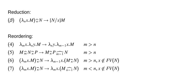
The reduction rules for this calculus are given in Figure 1. -Reduction only happens
Reduction:
() (px:M) bpN
![N=x]M
Reordering:
(1) px:qy:M!qy:px:M p>q (2) M
bpNbqP !M
bqPbpN p >q
(3) (px:M) bqN
!px:(M bqN
) p6=q; x62FV(N)
Figure 1. Reduction rules for symbolic selective-calculus
on abstraction-application pairs with the same label.3 Otherwise they commute by rule (3). Rules (1) and (2) simply normalize the order of abstractions and applications.
For convenience, we will sometimes use a variant syntax using record notation. A record is an expression of the form(p1)M1;. . .;pn)Mn)the pis are labels and the Mis are terms. We shall use these expressions with the following syntactic equivalence:
2It will be convenient, though not necessary, to assume that
is the least element ofS. 3The notation [N
=x]M denotes the term obtained from M after substituting all the free occurrences of variable x
(p1)x1;. . .;pn)xn):M
p1x1::p nxn:M M(p1)M1;. . .;pn)Mn) (. . .(M
b
p1M1). . . b pnMn):
An example of reduction in the symbolic selective calculus is given in Figure 2
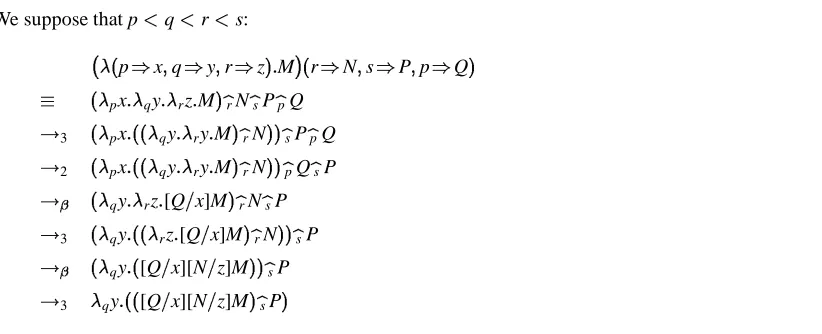
We suppose that p<q<r<s:
(p)x;q)y;r)z):M
(r)N;s)P;p)Q)
(px:qy:rz:M)
brNbsPbpQ !3 (px:((qy:ry:M)
brN ))
bsPbpQ !2 (px:((qy:ry:M)
brN ))
bpQbsP !
(qy:rz:[Q=x]M) brNbsP !3 (qy:((rz:[Q=x]M)
brN ))
bsP !
(qy:([Q=x][N=z]M)) bsP !3 qy:(([Q=x][N=z]M)
[image:15.612.93.504.140.307.2]bsP )
Figure 2. Example of reduction with symbolic labels
We call symbolic selective-calculus the free combination of these rules and-conversion.
Theorem 1 The symbolic selective-calculus is confluent.
Proof: Consequence of the proof for selective-calculus, in [2]
4 -Calculus with relative positions
This calculus is very similar to the previous one. Its syntax is identical; the only difference is that the labels are positive natural numbers:
M::=x jn:MjM bnM
0
where n2N IN f0g.
Again, for compatibility with the classical-calculus, we shall use position 1 as default. That is, any unlabeled abstraction or application is interpreted as being labeled by 1. In other words, classical-calculus is the special case whenN =f1g.
The reduction rules are also similar, but with a twist. They are are given in Figure 3. The main idea here is to preserve coherence between argument position numbers and the property used for currying that all functions are unary. Hence, it is necessary to adjust a position number relatively to the form on its left.
Reduction:
() (nx:M) bnN
![N=x]M
Reordering:
(4) mx:ny:M!ny:m 1x:M m>n (5) M
b
mNbnP
!M bnP
d
m 1N m>n
(6) (mx:M) bnN
!m 1x:(MbnN) m>n;x62FV(N) (7) (mx:M)
bnN
!mx:(M c
[image:16.612.111.517.65.238.2]n 1N) m<n;x62FV(N)
Figure 3. Reduction rules for numerical selective-calculus
of arguments of lesser position indices on its left. More precisely, let(n1)M1;. . .;nk)Mk) be a record expression where ni 2 N for i = 1;. . .;k. Then, for any i = 1;. . .;k in this expression, its relative position offset is the number o(i)of labels in the setfn1;. . .;ni 1gthat are strictly less than ni. For example, the relative position offsets of the record expression:
(4)M1;1)M2;5)M3;2)M4;2)M5)
are: o(1)=0;o(2)=0;o(3)=2;o(4)=1;o(5)=1. Hence, the syntactic equivalence is given by:
(n1)x1;. . .;nk)xk):M n
1x1:. . .:
nk o(k)xk :M M(n1)M1;. . .;nk)Mk) (. . .(M
b
n1M1). . . d nk o(k)Mk
):
An example of reduction in the numerical selective calculus is given in Figure 4 Theorem 2 The numerical selective-calculus is confluent.
Proof: Consequence of the proof for selective-calculus.
5 The selective-calculus
The selective-calculus combines orthogonally the symbolic and the numerical selective -calculi by usingL=SN as set of labels.
4 Thus its syntax is: M::=xj
` :MjM
b `M
0
where`=pn2L=SN.
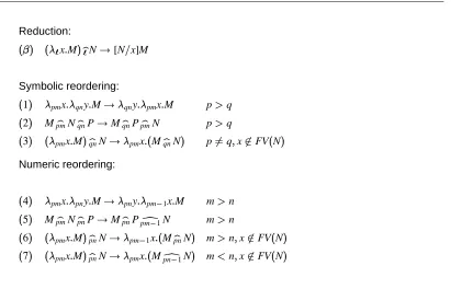
The reduction system is the combination in Figure 5. Applying these rules simply amounts to applying independently the symbolic and numeric systems. One may see reordering rules as structural equalities, and -reduction as unique reduction rule. Since the combination is orthogonal, it inherits confluence from both systems.
4In [2] this particular variant was defined as a product system, and what we called there selective
-calculus as
((2)x;1)y;4)z):M)(4)N;6)P;2)Q)
(2x:1y:2z:M)
b4Nb5Pb2Q !4 (1y:1x:2z:M)
b4Nb5Pb2Q !7 (1y:((1x:2z:M)
b3N ))
b5Pb2n3 !5 (1y:((1x:2z:M)
b3N ))
b2Qb4P !7 (1y:1x:((2z:M)
b2N ))
b2Qb4P !
(1y:1x:[N=z]M) b2Qb4P !7 (1y:((1x:[N=z]M)
b1Q ))
b4P !
[image:17.612.92.504.94.277.2]
(1y:[Q=x][N=z]M) b4P !7 1y:([Q=x][N=z]Mb3P)
Figure 4. Example of reduction with numeric labels
Reduction:
() (`x:M) b`N
![N=x]M
Symbolic reordering:
(1) pmx:qny:M!qny:pmx:M p>q (2) M
b
pmNqnbP
!M b
qnPpmb N p
>q
(3) (pmx:M) b
qnN!pmx:(M
b
qnN) p6=q;x62FV(N)
Numeric reordering:
(4) pmx:pny:M!pny:pm 1x:M m>n (5) M
b
pmNpnbP
!M b
pnPpmd1N m
>n
(6) (pmx:M) b
pnN!pm 1x:(M
b
pnN) m>n;x62FV(N)
(7) (pmx:M) b
pnN!pmx:(M
d
pn 1N) m<n;x62FV(N)
[image:17.612.96.507.348.612.2]Theorem 3 The selective-calculus is confluent.
Proof: This is a consequence of the proof for the sum system in [2]. We extend easily the use of numerical indices, which can be seen as being limited to a only one keyword in the sum system, to all keywords thanks to channel independence.
To let this system include the symbolic calculus and numerical calculus as sub-calculi, we will identify a symbolic keyword p in the former with the label(p;1), and a numeric index n in the latter with the label(;n). Thus, the classical unlabeled-calculus is also syntactically embedded in selective-calculus by taking(;1)as the default label of all abstractions and applications.
6 Simple types
As in classical -calculus, we introduce simple types. There are two benefits. First, we gain a better understanding of the label-selective calculus itself by explicating the type structure that it needs. Second, simply typed selective-calculus gains the same nice expected properties; e.g., strong normalization of well-typed terms.
6.1 Syntax and types
The original syntax of terms is extended to: M::=xj
`x : t :MjM
b `M
0 :
which requires abstracted variables to be explicitly typed.
We define the syntax of label-selective simple types with the following grammar:
` ::= pn (labels) u ::= u1ju2j. . . (base types) r ::= f`)t;. . .g (record types) t ::= ujr !u (general types)
where the expressionf`)t;. . .gdenotes a finite partial function fromL to types, including the empty functionfg. We shall identify a functional type of the formfg! u with the base type u. Note that record types are not types of expressions of our term language. They are used exclusively as the left subexpression of function types.
The idea behind this syntax of types is to convey that an application can be done indifferently through any label that is present in the type, on a value of corresponding type. 6.2 Record concatenation
To simplify the discussion, let us first restrict ourselves to numeric labels only. Consider the two record types r = f2)t1;4)t2gand s= f2)u1;3)u2g. Extending the type r on the right with s must be done such that the relative positions be kept in coherence. Now, r expects t1 in second position and t2in fourth position. In other words, positions 1, 3, 5 and up, are “free” in r in the sense that if more arguments were to be expected by an extension of r, they could use these free slots in sequence. Consider now extending r with s. The first argument’s position in s is 2. Hence, in r’s context, this argument corresponds to the second “free” slot; i.e., position 3. The following one in s is in position 3, and hence corresponds to the third “free” slot in r; i.e., position 5. Thus, the record type resulting from the concatenation of r and s is rs=f2)t1;3)u1;4)t2;5)u2g.
The case of multiple channels is not more complicated since the above scheme is to be used on each channel independently. Intuitively, this operation reminds of stream merging. In fact, this is exactly what is happening as the indices on a given channel in a record indicate the expected positions, but only relative to this specific record. Extending the record with more indices on this channel necessitates adjusting the new indices by taking their positions with respect to the sequence of indices unused by the initial record. We now proceed to defining formally this record-type concatenation operation.
Let r=f`1)t1;. . .;`n)tngbe a record type. We shall denote byDr =f`1;. . .;`ngthe set of labels defined in r. Recall that our record labels are not simple symbols, but pairs of the form pn, a symbol and a position index.
Definition 1 (occupied position) The nth position on p in a record type r is said to be occupied if r is such that pn2Dr.
Given a record type r, we denote by or(pn)the offset of n on p in r to be the number of occupied positions on symbol p in r with index less than or equal to n. That is, or(pn)=j(fpg[1;n])\Drj.
For example, consider the two following record types:
r=fp2)t1;p4)t2;q1)t3;q2)t4;q5)t5g; s=fp2)u1;p3)u2;q2)u3;q3)u4g:
The offsets of the labels of s in r are, respectively, or(p2)=1, or(p3)=1, or(q2)=2, and or(q3)=2.
Given a record type r and a given symbol p, we need to identify the least index of p in r that is not an occupied position. More precisely, it is useful to know the nth such free position for symbol p in r.
Definition 2 (free position) The nth free position for p in r is given by:
r ;p
(n)=minfi2N ji or(pi)=ng:
For example, given the previous example’s two record types, the free positions in r available for the indices in s are, respectively,r
;p
(2)= 3, r ;p
(3)= 5,r ;q
(2)= 4, and r
;q
For fixed r, this function is extended to work also on a record type by distributing it on each label. Namely, for any s=fpini)tig
k i=1
,r(s)=fpir ;pi
(ni))tig k i=1
.
For example, for r and s used above: r(s)=fp3)u1;p5)u2;q4)u3;q6)u4g. It is not coincidental that the label domain of ther(s)is disjoint from that of r. It is easy to show that this is true in general.
Definition 3 (concatenation) Record-type concatenation is defined as rs=r]r(s), where
]denotes union of functions with disjoint domains.
Going back to the two record types r and s used in the examples above, we have rs = fp2)t1;p3)u1;p4)t2;p5)u2;q1)t3;q2)t4;q4)u3;q5)t5;q6)u4g:
Proposition 4 Label-selective record-types form a monoid; i.e., concatenation is associative with neutral elementfg.
Proof: This is becauser s
=rs(see appendix). 6.3 Record matching
It is essential for a syntax-directed inference system, like the typing system that we are about to give, to be able to solve syntactic equations of the form rx=s. More specifically, to extract a subexpression r out of a record type expression it is convenient to write the latter as r]s (i.e., splitting it), and let that be the result of an expression rx, solving for x.
Remarkably, there is an inverse to record-type concatenation that allows solving such an equation and thus may be used to identify a given record type as the result of the concatenation of two other record types. We call this operation record-type matching.5 It will be used with great benefit in typing rules as well as for polymorphic type unification and type inference as shown in the next section.
Let r and s be two record types with disjoint label domains (i.e., such as could be obtained by partitioning one into two). Let pi be a label in s. For p, the position i can be seen as the result of having concatenated r with the same type originally at position i or(pi). In fact, for all the label indices i of p in s, this defines an inverse function forr
;pas
1 r;p
(i)=i or(pi). That is,
1 r;p
(i) computes the index corresponding to i on channel p skipping the occupied positions on p in r that are less than or equal to i.
As before, for fixed r,
1is extended to record types. Namely, for any s
=fpini)tig k i=1 such that pini62Drfor all i=1;. . .;k,
1
r (s)=fpi 1 r;pi
(ni))tig k i=1.
Definition 4 (matching) Record-type matching is defined as r]s = r 1
r (s), where ] denotes union of functions with disjoint domains.
Let r = fp1)t1;q2)t2g and s = fp2)u1;q3)u2g. The unique solution to the matching equation r]s=rx is x=
1
6.4 Typing rules
We now have all we need to define well-typedness. We will denote by a typing environment; i.e., a mapping from term variables to types. The notation [x7!] denotes the typing environment that coincides with everywhere, except on x for which it gives the type .
Definition 5 A term M is well-typed if there is a mapping from the free variables of M to types and a type such that `M : is derivable in the type inference system of Figure 6.
[x7!]`x : (I)
[x7!]`M : r!
``x : :M :fl) gr!
(II)
`M :f`) gr! `N :
`M b `N : r
!
[image:21.612.90.497.203.346.2](III)
Figure 6. Typing of simply-typed label-selective calculus
Simply typed selective -calculus verifies the two fundamental properties of typed -calculi.
Proposition 5 (subject reduction) Reduction preserves the types; i.e., if ` M : and M!N then `N :.
Theorem 6 (strong normalization) The simply-typed label-selective -calculus is strongly normalizing.
7 Polymorphic selective-calculus
While there exist typing systems that are more powerful than ML’s (e.g., second-order polymorphic-calculus), the style of polymorphism used in ML is much simpler. This is essentially due to restricting type quantification to appear only at the outset of type expressions, which facilitates type instantiation to be done implicitly following applications. The main advantage of this type system is that, for -calculus, any term has a principal (i.e., most general) type that can be reconstructed from the shape of the term alone. This obviates explicit type declarations: a simple type unification algorithm synthesizes missing types.
7.1 Syntax and types
The syntax is that of untyped selective -calculus with a let construct to introduce polymorphism, types being provided by inference. Thus, the syntax of terms is given by:
M::=xj `x
:MjM b `M
0
jlet x=M in M 0
and the reduction rule corresponding to the new construct is:
let x=M in N![x=M]N:
As in Damas and Milner’s definition [8], types are partitioned into monotypes, ranged over by t, and polytypes, ranged over by. Thus, the language of types is given by:
w ::= ujv (return types) r ::= f`)t;. . .g (record types) t ::= wjr!w (monotypes)
::= tj8v: (polytypes)
where return types u stand for base types and v for type variables. Here again, record types are not types of expressions of the term language.
7.2 Type substitution
The distinction we introduce here between return types and monotypes is specific to selective-calculus. Indeed, as we shall see, the main difficulty in our system, when compared to -calculus with ML-style polymorphic types, is that function types are always kept flat. Observe, indeed, that function types are not return types. For example,f`)g ! (f`
0 )
g!)is not a valid type expression in our type language. It is possible, however, to obtain such an expression as the result of substituting a valid type for a type variable in another valid type. For example, doing a direct substitution withf1)g!for in typef1)g ! would result inf1)(f1)g!)g!(f1)g!). This means that when we substitute a variable that appears as return type with a functional type, we will need to modify the structure of the type.
The solution is to define type substitution with a built-in flattening of the domain type. We will denote this operation as [
0
n] (i.e., substitute type 0
for type variablein) and it is performed as expressed by the following simple rule:
[(r 0
!!)n](r!)= ([(r 0
!!)n]r)r 0
!!:
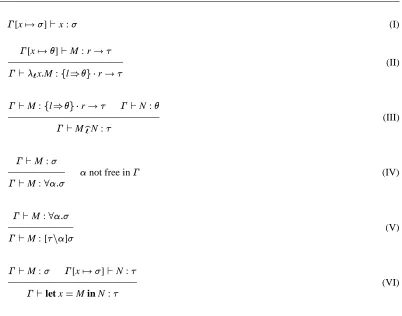
7.3 Typing rules
The typing rules are given in Figure 7. It is interesting to remark that Rules (IV)–(VI)
[x7!]`x : (I)
[x7!]`M : r!
``x:M :fl) gr!
(II)
`M :fl) gr! `N :
`M b `N :
(III)
`M :
`M :8:
not free in (IV)
`M :8:
`M : [n]
(V)
`M : [x7!]`N :
`let x=M in N :
[image:23.612.101.503.102.418.2](VI)
Figure 7. Typing rules for polymorphic selective-calculus
are in no way specific to selective -calculus. Since type quantifiers are external, they are independent of the structure of monotypes. Thus, these rules are exactly the same used in classical -calculus. Their roles are generalization (IV), instantiation (V), and let-introduction (VI). The only, but important, difference between these rules and the classical ones is hidden in the use of our flattening type substitution [n]in Rule (V).
Again, all the desirable properties hold for the polymorphically typed selective-calculus, as expressed by the two following propositions.
Proposition 7 (subject reduction) If ` M : in polymorphically typed selective -calculus, and M!N, then `N :.
Theorem 8 (strong normalization) Polymorphic selective-calculus is strongly normaliz-ing.
7.4 Type unification
problem [11], where the equational theory is that deciding equality of record types. Then, our type substitution operation using record-type concatenation constitutes a complete set of reduction for this theory. We next give this unification procedure as a complete set of equivalence-preserving transformations on a set of type equations.
A set of type equations 'is said to be in solved form if every equation in it is of the form = such that the type variable occurs only once in '; viz., as this equation’s lefthand-side. As usual, such a solved-form defines a variable substitution that can be applied to type expressions.
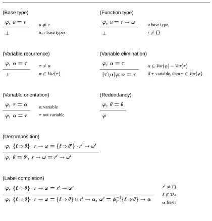
Figure 8 contains the complete set of transformations for the unification of label-selective monotypes. We use the notation for type variables,! for return types, and orfor any type expression. (Again,fg!!is identified with!.)
These rules work on a set (a conjunction) of type equations, transforming it into another such set. Upon termination, having started from a set 'of equations, the resulting equation set is either?, the inconsistent equation indicating that no solution exists, or sol('), a set of equations in solved form equivalent to'.
In either case, this process can be seen as returning a substitution. In the first case, it is the failing substitution?such that?()=?for all types, where?denotes the inconsistent type. In the second case, the solved form sol(')is the most general unifier (MGU) of'(up to variable renaming). The rules are written as rewrite rules using a comma as an associative and commutative set constructor, and the equal sign as a symmetric equation constructor. That is, in these rules the particular order of equations in the set as well as the orientation of an equation are irrelevant. As established by the following theorem, they are solution-preserving and there is a deterministic strategy that makes them always terminate.
Theorem 9 (label-selective type unification) There is an algorithm that computes the most general unifier of a set of equations on monotypes or reports failure if there is none.
7.5 Type inference
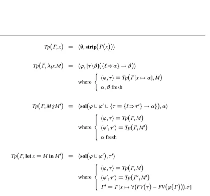
It is now easy to derive a type inference algorithm by combining type unification with the typing rules of Figure 7. It is sufficient to following the syntactic structure of a given term, accumulating new equations in a set, as shown in Figure 9. The function Tp takes a typing environment (a function from term variables to types) and a selective-term M, and returns a pairh';iwhere'is a set of type equations in solved form (i.e., a type substitution), and is the principal type of M. The function strip applies to a type expression81:8n:, where n0, and returns the expression obtained from where all theis, if any, are replaced with fresh names.6 The expression FV()is the set of free variables in, and by extension FV( ) =
S
xFV( (x)). The expression sol('), where ' is a set of type equations, is the solved form of ' (i.e., the MGU of'). It is the result of applying the transformation rules of Figure 8 to ' until none applies. The expression '() is the result of applying the substitution' to the type expression. By extension, '( )is the function defined by '( )(x)='( (x)).
This algorithm constructs a derivation tree whose root is `M :, where and M are given. Since there is only one way to construct this tree, by induction on the structure of M,
6If n
(Base type)
'; u=v
?
u6=v
u;v base types
(Variable recurrence)
'; =
?
6=
2Var()
(Variable orientation) '; = '; = variable not variable (Function type)
'; u=r!!
?
u base type
r6=fg
(Variable elimination)
'; =
[n]';=
2Var(') Var()
if variable, then2Var(')
(Redundancy)
'; =
'
(Decomposition)
'; f`) gr!!=f`) 0
gr 0
!! 0
'; = 0
; r!!=r 0
!! 0
(Label completion)
'; f`) gr!!=r 0
!! 0
'; f`) gr!!=f`) g]r 0 !; ! 0 = 1 r0
f`) g!
r0 6=fg
`62Dr 0
[image:25.612.84.504.125.563.2]fresh
Tp( ;x) = h;;strip( (x))i
Tp( ; `x
:M) = h';[n](f`)g! )i
where 8 <
:
h';i=Tp( [x7!];M) ;fresh
Tp( ;M b `M
0
) = hsol('[' 0
[f =f`) 0
g!g);i
where 8 > > > < > > > :
h';i=Tp( ;M)
h' 0
; 0
i=Tp( ;M 0
)
fresh
Tp( ;let x=M in M 0
) = hsol('[' 0 ); 0 i where 8 > > > < > > > :
h';i=Tp( ;M)
h' 0
; 0
i=Tp( 0
;M 0
)
0
= [x7!8 FV() FV('( ))
[image:26.612.105.524.115.507.2]:]
this algorithm is complete and correct. This is because only necessary equations are added, except for generalization and instantiation, which are handled in the most general way in the variable and let cases.
8 Conclusion and further work
We have proposed two typing systems for label-selective-calculus: simple types and ML-style polymorphic types. The latter are smoothly accommodated thanks to the existence of a simple but flexible record-type concatenation operation that facilitates building label-selective currying right into type substitution and unification. Integrated into a polymorphic functional programming language with currying, this provides a powerful tool, extending currying facilities and helping to memorize multi-argument functions.
An interesting subject is how to mix record operations and selective-calculus. The idea comes from the natural encoding of records in the untyped calculus, as:
f`1)a1;. . .;`n)ang !sels:(s b `1a1. . .
b `nan
)
where sel is a distinguished fixed channel and s is a function selecting a label and discarding the others individually (we have no way to discard them at once), like
`1x1 :. . .:
`nxn :xk. We can even have functions using more than one label. This is in fact the basic idea for a transformation calculus. However, there are some essential differences between a classical definition of records and this encoding as it accommodates numerical indices. We suspect that type inference of such a calculus with useful operations might turn out to be rather complex.
Another application of this calculus might be found in parallel processing. If we now see labels on a stream as identifying threads, the commutation capability directly interprets a concurrent evaluation. This is an idea very close to the dataflow paradigm, but we hope to replace flow analysis by type synthesis. Another, but not contradictory, view is to see labels as names, like for process communication. It shows a link, which can easily be made more evident, with calculi like Milner’s-calculus [16]. The conjunction of those two views seems an interesting prospective.
Appendix: Proofs of theorems
Proposition 4 Record-type concatenation is associative.
Proof: Let us show thatrs=r
]r(s). We proceed with inverses:
1
r]r(s);p
(i)=i or ]r(s)
(pi)
=i or(pi) os(
1
r;p
(i))
=
1
s;p
(
1
r;p
(i)):
We then have:
r(st)=r]r(s]s(t)) =r]r(s)]r(s(t)) =r]r(s)]r
]r(s) (t)
=(rs)t:
Proposition 5 (subject reduction) If `M : and M!N then `N :.
Proof: We only need to prove this property when M is a redex and N is the result of this reduction. We can then generalize by substitution and repetition.
If M is a-redex, it is of the form(`x : :P) b
`Q. Then, the basis of the proof tree is:
[x7!]`P : r!
``x : :P :fl) gr!
`Q :
`M : r!
After reduction the result is N=[x=Q]P. We obtain a derivation tree for `[x=Q]P from those
of [x7!]`P : r! and `Q :as follows: (1) doing all-conversions necessary to the
substitution of x by Q; (2) suppressing x in the environments (except where it is redefined by an abstraction); (3) where x appears without being defined in the environment, replacing 0
`x :by
the derivation tree of 0
`Q :. This poses no problem since8y2FV(Q) (y)= 0
(y).
If the reduction is a reordering, we have seven cases. We will only work out in detail cases (3), (6) and (7).
Case (3): If the reduction is (3), then the derivation tree must have the following form:
[x7!]`M :fqn) 0
gr!
`pmx : :M :fpm) ;qn)
0
gr!
`N : 0
`(pmx : :M)
b
qnN :fpm) gr!
[x7!]`M :fqn) 0
gr! [x7!]`N : 0
[x7!]`M b
qnN : r!
`pmx : :(M
b
qnN):fpm) gr!
Case (6): If the reduction is (6), then n<m, and the derivation tree must have the following form:
[x7!]`M :fpn) 0
gr!
`pmx : :M :fpn)
0
;pm) gr!
`N : 0
`(pmx : :M)
b
pnN :fp(m 1)) gr!
Since x62FV(N), we can obtain the following derivation tree after reordering:
[x7!]`M :fpn) 0
gr! [x7!]`N : 0
[x7!]`M b
pnN : r!
`p (m 1)x :
:(M b
pnN):fp(m 1)) gr!
Case (7): If the reduction is (7), then m<n, and the derivation tree must have the following form:
[x7!]`M :fp(n 1)) 0
gr!
`pmx : :M :fpm) ;pn)
0
gr!
`N : 0
`(pmx : :M)
b
pnN :fpm) gr!
Since x62FV(N), we can obtain the following derivation tree after reordering:
[x7!]`M :fp(n 1)) 0
gr! [x7!]`N : 0
[x7!]`M d
p(n 1)
N : r!
`pmx : :(M
b
pnN):fpm) gr!
Theorem 6 The simply typed selective-calculus is strongly normalizing.
Proof: The idea is to construct a function that gives the longest reduction of a term in function of its input. By reduction steps, we only mean here-reductions, since we already know that reordering
is Noetherian.
First, let us define zero functions, and the operation of rectification of a function. In fact, we use
notation since we know that selection is deterministic by the confluence theorem, and we could translate them to classical functions using their types and the order on labels.
Let = f`1)1;. . .;`n)ng ! u be a simple type. The zero-function for, noted0
, is the function(`1)x1:
1;. . .;`n)xn:
n):0, of type
, where is defined by induction as (f`1)1;. . .g!u)
=f`1)
1;. . .g!int (we replace every base type with int).
To rectify a function f of type =f`1)1;. . .;`n)mgr!u to r!u one simply applies it to
the corresponding zero-functions: rect(r!u;f :)=f(`1)0 1
;. . .;`n)0 n
).
We define our function T (M)by induction on the structure of the term M, annotated with types in
some typing environment . We suppose that keywordsSand variablesV are independent, and
useV[Sas symbols for the respective selective functions.
For a variable `x :, the associated function isxx :
:x.
For an abstraction ``x : :M :fl) gr!, the associated function is`x :
:T [x 7!]
(M).
For an application `M b `N : r
!, with `N :, the associated function is: T (M
b `N
)=x
1x1::x
nxn: (T (M) b
x1x1. . .bxkxk b `
Na)+ rect(int;N
a:
)+1
where:
1. FV(N)=fx1;. . .;xng;
2. FV(M)\FV(N)=fx1;. . .;xkg,0kn;
3. Na
=T (N) b
x1x1. . . bxnxn;
4. for f :f`1)1;. . .;`n)ng!int and a : int,
f + a=(`1)x1:1;. . .;`n)xn:n):(f(`1)x1;. . .;`n)xn)+ a):
This sum of three terms expresses that N may be reduced after substitution in M, or before, and that there may be one step of-reduction.
In this function we make two approximations. The first one is that we count one step for each application, whether or not there is an abstraction to reduce. The second one is that we take the sum of the call-by-name and call-by-value strategies, and not their maximum. Since these are only over-estimations, our function gives an upper-bound of the longest reduction path.
If `M :f`1)1;. . .;`n)ng! and jFV (M)
=fx17!1;. . .;xm7!mg, then T (M)is a
total function from 1 n 1
mto int. This means that on any complete input that
is coherent with its typing, M will terminate. Moreover, an upper bound of its longest reduction path is given by rect(int;T (M):(r!)
).
Proposition 7 (subject reduction) If ` M : in polymorphically typed selective -calculus, and M!N then `N :.
Proof: Since polymorphism can only be used in conjunction with let, the proof for simple types is enough except for let-reduction.
In this last case, the derivation tree starts with:
`M : [x7!]`N :
We first perform all-conversions necessary to the substitution of x by M. After reduction, we
obtain a tree with root `[x=M]N : from the derivation tree of [x7!]`N : by replacing
every occurrence of the axiom 0
[x7!]`x :by the derivation tree of 0
`M :; observing
that8y2FV(M) (y)= 0
(y).
Theorem 8 Polymorphic selective-calculus is strongly normalizing.
Proof: We find an upper bound of the longest evaluation of M by that of ˜M, which is M where
all occurrences of let are suppressed by transforming let x=P in N into K b1
([x=P]N)
b1P, where K = 1x:1y:x. We need K for the case where x does not appear in N. Since the result is
monomorphic everywhere, the argument for the simply typed calculus holds.
Theorem 9 (label-selective type unification) There is an algorithm that computes the most general unifier of a set of equations on monotypes or reports failure if there is none.
Proof: We first prove the correctness of the rewriting system of Figure 8. That is, for each rewrite rule, any solution of the denominator is a solution of the numerator, and conversely, any solution of the numerator can be extended into a solution of the denominator, possibly by introducing new variables missing in the numerator.
The rules labeled Base type, Variable recurrence, Function type detect inconsistencies in the equations. That is, respectively, equation between two different base types, between a type variable and a type containing it, or between a base type and a functional type. When one of these rules applies, the system has no unifier.
The Variable elimination rule substitutes variables (using flattening type substitution), while keeping their referents. Letbe a solution of the numerator. Then, by construction, ()= (), thus it
is also a solution of the denominator; and conversely.
The Variable orientation rule simply reorients an equation. It is not really necessary and is provided only to obtain the solved form with all solved variables on the left. Clearly, it leaves unchanged the set of unifiers. So does the Redundancy rule which just suppresses tautological equations.
Decomposition takes a label already present on the two sides of an equation, and equates the types.
Correctness is clear.
Whenever a label appears only on one side of an equation, it is necessary to introduce it in the other side. This is done by the Label completion rule using record-type matching. Any unifier of the denominator is also a solution of the numerator, sincef`) g]r
0
!=r 0
1
r0
f`) g!,
which is by unification equal to r0 ! !
0
. Conversely, ifis a unifier of the numerator, then it
maps! 0
to a functional type of the form
1
r0
f`) ( )gr 00
!! 00
, which can be extended for the denominator by adding ()=r
00 !!
00
.
We next prove that there is a terminating strategy. Termination follows for the well-foundedness of a decreasing measure. A variable is solved when it appears only once, and as the lefthand-side of an equation. We exhibit a strategy that reduces the lexicographical measure (number of unsolved
variables,sum of sizes), where the size of a type is the total number of labels, variable occurrences
and base types it contains.
The three failing rules terminate. Redundancy, and Decomposition reduce the sum of sizes. Variable elimination and Variable orientation reduce the number of unsolved variables.
Label completion by itself does not reduce the measure. But if it is always used it in combination with Decomposition on the same equation, eliminating or failing as soon as possible, this always reduces the number of unsolved variables. If!
0
it is solved, but we create a new variable. We repeat this until we can solve a “successor” of
with the left hand side (which may suppose creating a lineage to!too, if completion is mutual).
This sequence terminates, since there is only a finite number of labels on each side.
Last, we must show that our result is in solved form. First, in every equation, at least one side is a solved variable. If the two sides are functional types, then either Decomposition or Completion applies. If one side is a base type, then the other side is a solved variable, otherwise Elimination, Redundancy or some failure applies. If the two sides are variables, then at least one is solved. We construct the substitutionby taking for each equation=,solved, () =. is a
most general unifier of the final system, and, as a consequence, if we suppress definitions for all variables introduced by completion,
0
References
1. Mart´ın Abadi, Luca Cardelli, Pierre-Louis Curien, and Jean-Jacques L´evy. Explicit substitutions. In Proceedings of ACM Symposium on Principles of Programming Languages, pages 31–46 (1990). 2. Hassan A¨ıt-Kaci and Jacques Garrigue. Label-selective -calculus. PRL Research report 31,
Digital Equipment Corporation, Paris Research Laboratory (May 1993).
3. Hassan A¨ıt-Kaci and Jacques Garrigue. Label-selective -calculus: Syntax and confluence. In Proceedings of the 13th International Conference on Foundations of Software Technology and Theoretical Computer Science (Bombay, India), LNCS 761. Springer-Verlag (December 1993).
4. Hassan A¨ıt-Kaci and Andreas Podelski. Towards a meaning of LIFE. Journal of Logic
Program-ming, 16(3-4):195–234 (July-August 1993).
5. Kim Bruce, Roberto Di Cosmo, and Giuseppe Longo. Provable isomorphisms of types. Technical Report LIENS-90-14, LIENS (July 1990).
6. Luca Cardelli. A semantics of multiple inheritance. Information and Computation, 76:138–164 (1988).
7. Luca Cardelli and Peter Wegner. On understanding types, data abstraction, and polymorphism.
Computing Surveys, 17(4):457–522 (1985).
8. Luis Damas and Robin Milner. Principal type-schemes for functional programs. In Proceedings of
ACM Symposium on Principles of Programming Languages, pages 207–212 (1982).
9. N. G. de Bruijn. Lambda calculus notation with nameless dummies, a tool for automatic formula manipulation. Indag. Math., 34:381–392 (1972).
10. Pierre Weis et al. The CAML Reference Manual, version 2.6.1. Projet Formel, INRIA-ENS (1990). 11. Jean Gallier and Wayne Snyder. Designing unification procedures using transformations: a survey. In Y. N. Moschovakis, editor, Logic from Computer Science, pages 153–215. Springer-Verlag (1989).
12. Jacques Garrigue. Label-selective-calculus. Rapport de D.E.A., Universit´e Paris VII (1992).
13. Lalita Jategaonkar and John Mitchell. ML with extended pattern matching and subtypes. In
Proceedings of ACM Conference on LISP and Functional Programming, pages 198–211 (1988).
14. John Lamping. A unified system of parameterization for programming languages. In Proceedings
of ACM Conference on LISP and Functional Programming, pages 316–326 (1988).
15. Henry Ledgard. ADA : An Introduction, Ada Reference Manual (July 1980). Springer-Verlag (1981).
16. Robin Milner. The polyadic-calculus: A tutorial. LFCS Report ECS-LFCS-91-180, Laboratory
for Foundations of Computer Science, Department of Computer Science, University of Edinburgh (October 1991).
17. Martin Odersky, Dan Rabin, and Paul Hudak. Call by name, assignment, and the lambda calculus. In Proceedings of ACM Symposium on Principles of Programming Languages, pages 43–56 (1993). 18. Atsushi Ohori. A compilation method for ML-style polymorphic records. In Proceedings of ACM
Symposium on Principles of Programming Languages, pages 154–165 (1992).
19. Didier R´emy. Typechecking records and variants in a natural extension of ML. In Proceedings of
20. R. Stansifer. Type inference with subtypes. In Proceedings of ACM Symposium on Principles of
Programming Languages, pages 88–97 (1988).
21. Guy L. Steele. Common LISP, The Language. Digital Press (1984).
22. Mitchell Wand. Complete type inference for simple objects. In Proceedings of IEEE Symposium
The following documents may be ordered by regular mail from: Librarian – Research Reports
Digital Equipment Corporation Paris Research Laboratory 85, avenue Victor Hugo 92563 Rueil-Malmaison Cedex France.
It is also possible to obtain them by electronic mail. For more information, send a message whose subject line [email protected], from within Digital, todecprl::doc-server.
Research Report 1: Incremental Computation of Planar Maps. Michel Gangnet, Jean-Claude Herv ´e, Thierry Pudet, and Jean-Manuel Van Thong. May 1989.
Research Report 2: BigNum: A Portable and Efficient Package for Arbitrary-Precision
Arithmetic. Bernard Serpette, Jean Vuillemin, and Jean-Claude Herv´e. May 1989.
Research Report 3: Introduction to Programmable Active Memories. Patrice Bertin, Didier Roncin, and Jean Vuillemin. June 1989.
Research Report 4: Compiling Pattern Matching by Term Decomposition. Laurence Puel and Asc ´ander Su ´arez. January 1990.
Research Report 5: The WAM: A (Real) Tutorial. Hassan A¨ıt-Kaci. January 1990.y
Research Report 6: Binary Periodic Synchronizing Sequences. Marcin Skubiszewski. May 1991.
Research Report 7: The Siphon: Managing Distant Replicated Repositories. Francis J. Prusker and Edward P. Wobber. May 1991.
Research Report 8: Constructive Logics. Part I: A Tutorial on Proof Systems and Typed
-Calculi. Jean Gallier. May 1991.
Research Report 9: Constructive Logics. Part II: Linear Logic and Proof Nets. Jean Gallier. May 1991.
Research Report 10: Pattern Matching in Order-Sorted Languages. Delia Kesner. May 1991.
y
Research Report 12: Residuation and Guarded Rules for Constraint Logic Programming. Gert Smolka. June 1991.
Research Report 13: Functions as Passive Constraints in LIFE. Hassan A¨ıt-Kaci and Andreas Podelski. June 1991 (Revised, November 1992).
Research Report 14: Automatic Motion Planning for Complex Articulated Bodies. J ´er ˆome Barraquand. June 1991.
Research Report 15: A Hardware Implementation of Pure Esterel. G ´erard Berry. July 1991.
Research Report 16: Contribution `a la R ´esolution Num ´erique des ´Equations de Laplace et
de la Chaleur. Jean Vuillemin. February 1992.
Research Report 17: Inferring Graphical Constraints with Rockit. Solange Karsenty, James A. Landay, and Chris Weikart. March 1992.
Research Report 18: Abstract Interpretation by Dynamic Partitioning. Fran¸cois Bourdoncle. March 1992.
Research Report 19: Measuring System Performance with Reprogrammable Hardware. Mark Shand. August 1992.
Research Report 20: A Feature Constraint System for Logic Programming with Entailment. Hassan A¨ıt-Kaci, Andreas Podelski, and Gert Smolka. November 1992.
Research Report 21: The Genericity Theorem and the Notion of Parametricity in the
Poly-morphic -calculus. Giuseppe Longo, Kathleen Milsted, and Sergei Soloviev. December
1992.
Research Report 22: S ´emantiques des langages imp´eratifs d’ordre sup ´erieur et interpr ´etation
abstraite. Fran¸cois Bourdoncle. January 1993.
Research Report 23: Dessin `a main lev ´ee et courbes de B ´ezier : comparaison des
al-gorithmes de subdivision, mod´elisation des ´epaisseurs variables. Thierry Pudet. January
1993.
Research Report 24: Programmable Active Memories: a Performance Assessment. Patrice Bertin, Didier Roncin, and Jean Vuillemin. March 1993.
Research Report 25: On Circuits and Numbers. Jean Vuillemin. November 1993.
Research Report 26: Numerical Valuation of High Dimensional Multivariate European
Secu-rities. J ´er ˆome Barraquand. March 1993.
Research Report 29: Real Time Fitting of Pressure Brushstrokes. Thierry Pudet. March 1993.
Research Report 30: Rollit: An Application Builder. Solange Karsenty and Chris Weikart. April 1993.
Research Report 31: Label-Selective-Calculus. Hassan A¨ıt-Kaci and Jacques Garrigue. May 1993.
Research Report 32: Order-Sorted Feature Theory Unification. Hassan A¨ıt-Kaci, Andreas Podelski, and Seth Copen Goldstein. May 1993.
Research Report 33: Path Planning through Variational Dynamic Programming. J ´er ˆome Barraquand and Pierre Ferbach. September 1993.
Research Report 34: A penalty function method for constrained motion planning. Pierre Ferbach and J ´er ˆome Barraquand. September 1993.
The
T
y
pe
d
P
ol
y
m
orphi
c
L
a
b
e
l-S
e
le
c
tiv
e
-Calcu
lu
s
J
a
c
ques
Garrigue
and
Has
s
a
n
A
¨ıt-Ka
ci
d i g i t a l
PARIS RESEARCH LABORATORY