Localized Pseudo-Skeleton Approximation Method
for Electromagnetic Analysis on Electrically Large Objects
Yong Zhang and Hai Lin*
Abstract—In this paper, the localized pseudo-skeleton approximation (LPSA) method for electromagnetic analysis on electrically large structures is presented. The proposed method seeks the low rank representations of far-field coupling matrices by using pseudo-skeleton approximations (PSA). By using PSA, only part of the original matrix is needed to be calculated and stored which is very similar to the adaptive cross approximation (ACA). Moreover, rank approximation and index finding schemes are given to improve the performance of the method in this paper. Several numerical results are given to demonstrate that the proposed method performs better than the randomized pseudo-skeleton approximation (RPSA) and ACA.
1. INTRODUCTION
The method of moments (MoM) [1] is a very effective technique for modeling arbitrarily shaped electromagnetic scattering and radiation problems made of perfect electric conductors (PECs). However, MoM will result in a dense impedance matrix caused by non-locality property of the Green’s function. Consequently, the storage, impedance matrix fill-in, and matrix-vector multiplication operations are of O(N2) complexity, where N is the number of unknowns. A number of successful techniques have dramatically reduced memory and computational cost associated with the iterative solution of surface integral equations (SIEs). Among them, the multilevel fast multipole algorithm (MLFMA) [2], which is a representative one of physically related fast methods, has succeeded in reducing the numerical complexity of memory to O(N) and CPU time to O(NlogN). However, in the MLFMA algorithm, the formulation, implementation, and occasionally performance depend on a priori knowledge of the Green’s function.
Another family of fast algorithms is famous for its kernel-independent property and purely algebraic nature such as the ACA algorithm [3]. The ACA algorithm takes advantage of the rank-deficient nature of coupling matrix blocks representing well-separated MoM interactions. The algorithm fills the rows and columns iteratively until the convergence of the approximate relative error. Recently, skeleton based techniques have been investigated deeply [4–8] which try to seek the dominant elements to represent the original obese couplings. Among them, Randomised pseudo-skeleton approximation (RPSA) [7] is based on the PSA [8] of the matrix. In the matrix decomposition process, the working rows and columns are chosen randomly. However, the numerical example of RPSA proposed in [7] is too simple, and the overall performance is not studied to be compared to ACA.
In this paper, we propose an localized pseudo-skeleton approximation (LPSA) method which is also based on the PSA to perform the electromagnetic analysis on electrically large structures. Different from RPSA, the proposed method seeks a more effective way to approximate the rank of the compressed matrices and finds the most suitable indexes in the decomposition process. Moreover, several canonical numerical electromagnetic scattering examples are given to compare the efficiency and accuracy of LPSA with RPSA and ACA.
Received 6 July 2015, Accepted 25 September 2015, Scheduled 2 November 2015
* Corresponding author: Hai Lin ([email protected]).
2. MOM FORMULATION
In all of the integral equation based methods, the boundary conditions are firstly considered to formulate the integral equations. For simplicity, only EFIE is given in this work which states that the total tangential electric field should vanish on a conducting surface.
ˆ
t·
Sdr
¯I+ ∇∇
k2
g(r,r)·J(r) = i
kηˆt·E
inc(r) (1)
where Einc stands for the incident electric field, k the wavenumber, η the wave impedance, S the surface of the objects, ˆtthe tangential unit vector onS,r is the source point,rthe observation point,
J the unknown electric current on the surface, andg(r,r) =e−jk|r−r|/(4π|r−r|) the scalar Green’s function. In order to achieve a linear system, the Galerkin testing approach and Rao-Wilton-Glisson (RWG) [10] functions are used. If iterative solvers are adopted, fast algorithms can be performed to accelerate the matrix-vector product (MVP) which is the most time-consuming part in each iteration step. For simplicity, the MVP equation for fast algorithms can be written as follows:
ZI=ZnearI+ Zfar,∗I (2)
where Znear represents the near-zone interactions which are directly computed and stored, and Zfar,∗
stands for couplings betweens the far-field groups which will not be calculated and stored directly.
3. FORMULATIONS AND EQUATIONS
In this section, the basic principle of low rank representations for MoM is briefly introduced at first. Then, the PSA method is described in detail. Lastly, we introduce the main concepts of the localization for PSA.
3.1. Low Rank Representations
The matrix derived in MoM is known as dense matrix. However, because of the nature of the Green’s function, the matrix consists of many numerically rank-deficient sub-blocks. Namely, the dense matrix blocks representing the interactions between two well-separated groups can be accurately represented by a much-reduced set of column vectors. Therefore, the low-rank matrixZcan be approximated by a product of two much smaller sub-matrices U and V. Namely,
Zm×n≈Um×rVr×n (3)
whereris the rank and satisfiesrmandr n. Instead of storingm×nentries, the above low-rank decomposition technique only requires the storing ofr×(m+n) entries. Thus, the associated memory requirement can be reduced. Similarly, when the matrixZis directly applied to a vector (the product of a matrix and a vector), the computational complexity is m ×n. In contrast, we can first apply matrices V and thenU to the vector in sequence, then the associated complexity will also be reduced to r×(m+n).
3.2. Pseudo-Skeleton Approximation
According to the skeleton approximation method, there exists a nonsingular r×r submatrix ˆZin Z. Denote the columns and rows ofZcontaining the submatrix ˆZby C(with dimensions ofm×r) andR
(with dimensions of r×n), respectively. That is, the submatrix ˆZis the intersection ofCandR. Then it is easy to verify that
Z=CZˆ−1R (4)
This is called skeleton approximation. Unlike using an iterative approach in ACA, here we choose
The actual rankr ofZcan be revealed when calculatingG(pseudo inverse of ˆZ). Assume that ˆZ
can be decomposed as follows via singular value decomposition (SVD):
ˆ
Z=WSY (5)
where U, S, and V are p×p matrices; S is a diagonal matrix with nonnegative diagonal elements in decreasing order; the prime represents the operation of the complex conjugate transpose. A preset threshold can be used to further decrease the dimension ofW,Sand Y. The calculation of the pseudo inverse of ˆZis then straightforward:
ˆ
Z−1=YS−1W (6)
Since S is a diagonal matrix, the inverse of S is just the reciprocal of the diagonal elements. After doing these operations, we can easily obtain matrices U and V defined before by the following definitions:
U =CY
V=S−1WR (7)
3.3. Proposed Method
In [7], RPSA is proposed as a randomized version for the localization of PSA in the computational electromagnetic (CEM) area. The sampled rows and columns are selected in a random way while the sampling number p is chosen twice as the rank of the original matrix. However, the authors have not given the scheme to approximate the ranks of the matrices of different dimensions. Therefore, we propose a new localized pseudo-skeleton approximation (LPSA) method in this paper to solve these problems. The same as MLFMA, the proposed method is also based on multilevel octree structure. The coupling matrices between distant relative groups (they are far groups in this level while their parent groups are close to each other) will be compressed to save memory.
The first problem is how to give a reasonable approximation on the rank of the original matrix. As we know, the group dimension will increase as the level decreases. That is because the lower-level boxes in the octree have larger radius and elements. Therefore, the rank of larger-dimension matrix should also get larger. However, the distance between the distant relative groups in the lower-level groups is also much bigger than the higher-level one which means that the rank of the original matrix will also be smaller than the original dimension. According to the theoretical study in [9], the rank of 3D integral kernel can be described as
Rank3D ∼O(k0) (8)
where k0 is the wave number corresponding to a frequency being studied. Thus, it is straight forward
to give an approximation ofαk0dfor the rank of matrices, wheredis the diameter of the bounding box
of the corresponding octree group andα the ratio given by the users to control the accuracy. Moreover, we can also adopt the equation of truncation number in MLFMA structure [2] to further decrease the rank’s growth ratio. We can see that the rank will increase as the dimension of the matrix gets bigger. However, the growth ratio is so slow that the efficiency of the LPSA method can be kept for electrically large problems. The rank approximation formulation in this article is given below:
Rank≈k0d+ 2 ln(π+k0d) (9)
The process will not stop until theprows and columns are calculated and stored. This is very similar to the ACA method while the principle rows and columns can be chosen to compress the original matrix.
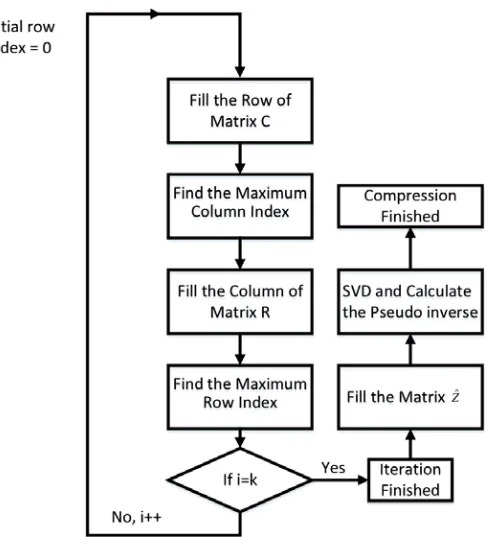
In summary, LPSA proposed in this paper can be readily implemented by the following steps:
1. p-Loop: Choose the working row and column to get part of the matrices Cand R. 2. Get the intersection matrix ˆZ.
3. Find the rank r by applying SVD to ˆZand get the submatricesU and V.
A flow chart is illustrated in Fig. 1 to help the readers to understand the implementation of the LPSA method.
Figure 1. The flow chart of the LPSA method.
4. NUMERICAL EXAMPLES
In this section, several experiments are given to show the efficiency of the proposed LPSA method. For all the simulations, the mesh sizes are about 0.1λ(λrepresents the wavelength), and the finest group is set to no less than 0.25λ. The biconjugate gradient stabilized method (BiCGSTAB) is adopted as the iterative solver for the matrix equations, and the threshold of the relative residual error is chosen as 0.003. All the computations were carried out on a workstation with four E5 4620 CPUs and 256 GB of RAM. The OpenMP technique and the double-precision digits are used in the calculation. Moreover, the sparse inverse approximate (SAI) [11] matrix is adopted as the preconditioner.
4.1. Accuracy
4.1.1. Fixed Rank Compared to RPSA
The first numerical example is given to demonstrate the fact that LPSA is more accurate than RPSA (the random indexes are generated once without refinement). The numbers of the sampled rows and columns are fixed as 2. In this way, the RCS values are plotted as Fig. 2.
Figure 2. LPSA and RPSA results for the sphere.
Figure 3. LPSA and ACA results for the sphere.
It is found that the RCS values obtained by LPSA are much closer to the Mie series than RPSA, which demonstrate the accuracy of the proposed method. LPSA performs better than RPSA since the largest entries are extracted by LPSA while the RPSA only selects the working rows and columns randomly. It is valuable to point out that the results of RPSA can be improved by increasing the value ofp and adding the refinement process at the price of ruining the computation efficiency. Compared to RPSA equipped with the refinement process, LPSA should be much faster with losing a little accuracy. Moreover, LPSA is also an error-controllable algorithm whose accuracy can be improved by increasing the number of working rows and columns.
4.1.2. Compared to ACA
Another comparison between LPSA and ACA is given in Fig. 3. In this example, the value ofα is set to 1.0.
It is demonstrated that the RCS curve obtained by the proposed LPSA method agrees well with the ones using ACA and Mie series.
Secondly, a larger aircraft model (JL-8A) is studied. The model is divided by a 6-level octree with 104169 unknowns. The incident plane wave angles satisfy θ= 0◦ and ϕ= 0◦ at 300 MHz. The bistatic RCS values inV-V polarization with pitch angles varying from 0◦ to 360◦ nd horizontal angle equal to 0◦ are calculated by LPSA, ACA and MLFMA.
From Fig. 4, it is obvious that the three RCS curves agree well with each other. Therefore, the three given scattering examples demonstrate that the proposed LPSA method is as accurate as the popular ACA and MLFMA methods.
4.1.3. Electrically Large Ship Model
Finally, an electrically large ship model is studied. The model is divided by a 8-level octree with 400374 unknowns. The incident plane wave angles satisfy θ = 0◦ and ϕ= 0◦ at 300 MHz. The bistatic RCS values in V-V polarization with pitch angles varying from 0◦ to 360◦ and horizontal angle equal to 0◦ are calculated by LPSA, ACA and MLFMA.
Figure 4. LPSA, ACA and MLFMA results for the aircraft.
Figure 5. LPSA, ACA and MLFMA results for the ship model.
4.2. Efficiency
In [7], the authors claimed that RPSA was faster than ACA while only a simple chart was given. In this section, the calculation time and memory usage are given based on several canonical examples.
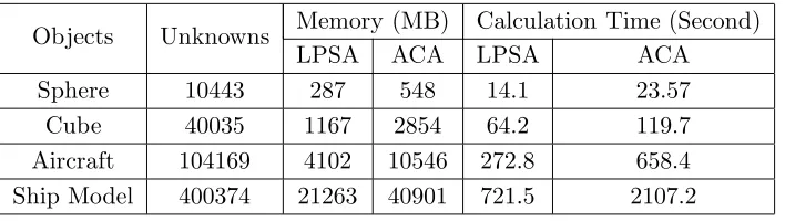
From the data listed in Table 1, the memory usage and calculation time of LPSA are both less than the ACA method. Thus, it is demonstrated that the computation cost for the same object of LPSA is lower than the ACA method without losing any accuracy.
Table 1. The unknowns and calculation statistics for different models.
Objects Unknowns Memory (MB) Calculation Time (Second)
LPSA ACA LPSA ACA
Sphere 10443 287 548 14.1 23.57
Cube 40035 1167 2854 64.2 119.7
Aircraft 104169 4102 10546 272.8 658.4
Ship Model 400374 21263 40901 721.5 2107.2
5. CONCLUSIONS
In this paper, we present a localized pseudo-skeleton approximation (LPSA) method for electromagnetic analysis on an electrically large structures. The proposed method seeks the low rank representations of far-field coupling matrices by localizing the pseudo-skeleton approximations (PSA) to EM simulations. In addition, the rank approximation and index finding schemes are given to improve the performance of the method in this paper. Some numerical results are also given to demonstrate the accuracy and efficiency of the proposed method.
ACKNOWLEDGMENT
REFERENCES
1. Harrington, R.,Field Computation by Moment Methods, Macmillan, New York, 1968.
2. Song, J. M. and W. C. Chew, “Multilevel fast-multipole algorithm for solving combined field integral equations of electromagnetic scattering,” Microwave Opt. Technol. Lett., Vol. 10, No. 1, 14–19, Sep. 1995.
3. Bebendorf, M., “Approximation of boundary element matrices,” Numer. Math., Vol. 86, No. 4, 565–589, 2000.
4. Brick, Y., V. Lomakin, and A. Boag, “Fast direct solver for essentially convex scatterers using multilevel non-uniform grids,”IEEE Trans. Antennas Propag., Vol. 62, 4314–4324, 2014.
5. Wei, J.-G., Z. Peng, and J.-F. Lee, “Multiscale electromagnetic computations using a hierarchical multilevel fast multipole algorithm,”Radio Science, Vol. 49, 1022–1040, 2014.
6. Pan, X. M., J. G. Wei, Z. Peng, and X. Q. Sheng, “A fast algorithm for multiscale electromagnetic problems using interpolative decomposition and multilevel fast multipole algorithm,”Radio Science, Vol. 47, RS1011, Feb. 2012.
7. Zhu, X. and W. Lin, “Randomised pseudo-skeleton approximation and its application in electromagnetics,” Electronics Letters, Vol. 47, No. 10, 590–592, 2011.
8. Goreinov, S. A., N. L. Zamarashkin, and E. E. Tyrtyshnikov, “Pseudoskeleton approximations by matrices of maximal volume,” Math. Notes, Vol. 62, No. 4, 515–519, 1997.
9. Chai, W. and D. Jiao, “Theoretical study on the rank of integral operators for broadband electromagnetic modeling from static to electrodynamic frequencies,” IEEE Transactions on Components, Packaging and Manufacturing Technology, Vol. 3.12, 2113–2126, 2013.
10. Rao, S. M., D. R. Wilton, and A. W. Glisson, “Electromagnetic scattering by surfaces of arbitrary shape,” IEEE Trans. Antennas Propag., Vol. 30, 409–418, May 1982.