University of Twente
EEMCS / Electrical Engineering
Control Engineering
Modelling and Distributed Controller Design
of the BodeRC Paper-path Setup
Frank Ambrosius
MSc Report
Supervisors:
prof.dr.ir. J. van Amerongen dr.ir. J.F. Broenink ir. P.M. Visser
January 2007
The BodeRC paper-path setup represents the paper transport path of a printer. It consists of a series of five pinches that transport a sheet of A4 size paper through the path. In this assignment a model and a control system of the paper-path have been designed such that the design trajectory as described in (Visser and Broenink, 2006) can be evaluated. The designed control system is capable of centralised control as well as distributed control. To get a structured approach in the design, the trajectory described by Broenink and Hilderink (2001) was followed. The first step in the trajectory is the design of a model of the physical system, the paper-path. This model was designed, verified with simulations and validated against experiment results on the setup. The results proved the correct functioning of the model. From the results it became clear that the paper detectors on the setup were not precise enough; A small alteration solved this problem.
Next, a control system has been designed. This system is capable of controlling the velocity of a sheet of paper throughout the entire paper-path. The control system relies on the presence of loop controllers for the pinches, which have been developed. The complete control system was evaluated, first in simulation together with the model then as embedded control system together with the paper-path setup. The resulting error is within the measurement resolution.
Finally, a distribution of the control system was designed. The distributed control system has been verified using simulations. The error proved to stay within the measurement resolution. Because the absence of software that handles the communication between nodes, the distributed control system could not be tested in practise.
Samenvatting
De BodeRC papierpad opstelling stelt het pad voor papier transport voor van een printer. Het systeem bestaat uit vijf knepen die A4 formaat papier voortstuwen. In deze opdracht zijn een model en een regelsysteem voor het papierpad ontworpen. Deze zijn zo ontworpen dat ze de evaluatie van het ontwerp traject als beschreven in (Visser and Broenink, 2006) ondersteunen. Het regelsysteem kan voor zowel gecentraliseerd als gedistribueerd regelen gebruikt worden. Om tot een gestructureerde aanpak te komen is het ontwerp traject beschreven door Broenink en Hilderink (2001) gevolgd.
De eerste stap in dit traject is het ontwerp van een model van het fysisch systeem, het paper-path. Dit model is ontworpen, geverifieerd met simulaties en gevalideerd tegen experimentele resultaten met de opstelling. Met deze resultaten is het correct functioneren van het model bewezen. Uit de resultaten blaak dat de papier detectoren op de opstelling niet nauwkeurig genoeg waren. Een kleine aanpassing heeft dit probleem opgelost.
Vervolgens is een regelsysteem ontworpen. Dit systeem is in staat de snelheid van het papier door het gehele pad te regelen. Het regel systeem heeft regellussen nodig voor de individuele knepen, deze zijn ontworpen. Het complete regelsysteem is ge¨evalueerd, eerst in simulatie samen met het model en vervolgens als embedded regelaar samen met de paper-path opstelling. De resulterende fout bleek kleiner dan de meetresolutie.
With this report I conclude my study in Electrical Engineering.
The past eight years have been a very valuable experience to me. I’ve learnt a great deal about myself and the the world around me. This learning process would not have been as much fun without the presence of friends and family. I would like to thank them for their support. Especially my parents, Piet and Greet, brother, Rob and girlfriend, Vanessa.
Further more I would like to thank Peter Visser and Jan Broenink for their supervision and support during my graduation project. Also my lab mates, Bert, Pieter and Ronald should receive thanks as should technician Gerben.
1 Introduction 1
C Experiments with centralised control 27 D Design trajectory 29 E Paper path setup specifications 30 F Pinch Modelling and Control Design 32 F.1 Modelling . . . 32
F.2 Model Verification and Validation . . . 35
F.3 Control Design . . . 37
F.4 Controlled System Simulation and Experiments . . . 39
F.5 Conclusions . . . 42
G How-To add a pinch to the plant model 44
Present day large scale projects such as the development of a high speed printer, rely on many disciplines. These disciplines traditionally use their own design methods and generally do not forsee the consequences for other parts of the system. To reduce the risk of a redesign step after system integration, the Embedded Systems Institute started the Boderc research project in 2002. In this research project several companies and universities work together to find a systematic approach for the development of distributed real-time embedded controllers for complex systems. The design approaches resulting from research at the University of Twente are verified using a demonstration setup that resembles a part of a paper path in a printer.
1.1
Previous work
This project supports the PhD. work of Visser (2007). The goal of this PhD. work is to develop a design trajectory for the design of distributed embedded control system software. Previous to this MSc. project, six BSc./MSc. projects were carried out in the scope of the Boderc project. The relevant parts of these projects are presented here.
1.1.1 Previous designed hardware and software
Otto (2005), designed a simplified version of the paper path of a printer. This paper path is shown in Figure 1.1. Combined with the embedded control system (Groothuis, 2004) it forms the paperpath setup (Figure 1.2) that can be used for testing the design approaches found. The tool-chain software for the complete system was designed in two other projects: (Buit, 2005) and (Posthumus, 2006). The setup shown consists of four parts that will be described below.
Distributed Embedded Control System This part contains a set of four embedded control systems (ECS). The ECS’s are embedded PC104 stacks each containing a processor board, a CAN interface board and an I/O interface board. The CAN bus is used for the commu-nication between nodes of a distributed control system. The I/O is used to connect the paper path under control to the ECS’s.
Hardware in the loop simulator A combination of one or more standard PC’s that can simulate a model (i.e. the paperpath setup) in real-time.
Paper path Mechanical setup, a simplified version of the Boderc test case printer.
Development Station A standard PC used for the design and deployment of the model and controllers to the Embedded Control System and the HIL simulator.
The Embedded Control System can be connected to either the Hardware in the loop simulator, for HIL simulations, or to the paperpath setup for real experiments.
Figure 1.1: Schematic overview of the Paper path (adapted from Otto, 2005)
Figure 1.2: Overview of the complete Paperpath Setup (adapted from Otto, 2005)
PIM The Paper Input Module consists of the input tray that holds the paper and two pinches that feed the paper into the path.
Output tray A bin that collects the paper after being fed through the path.
Sheet Detector Detect the presence of a sheet by the reflection of light emitted by the sensor.
Pinch The driving force of the paper path. Consists of a motor that is connected to a set of rubber wheels via a timing belt. These wheels can pinch a sheet and drive it through the path. The complete path has five pinches.
1.1.2 Previous designed models and controllers
Previous work on modelling a paper path has been done by van den Berg (2003) and by van Kampen (2003). In (van den Berg, 2003) the focus was on the logical state of the printer. Dynamics like slip and stick of paper and the response of the motors are not included. This enabled the simu-lation of the plant on a high level but does not facilitate simusimu-lation of the dynamics. To enable the simulation of these effects van Kampen (2003) describes a model that includes an extensive friction model. This model facilitates the simulation of a paper path to check for the effects of paper and motor dynamics on the performance of a printer. Although friction models are present, the dynamics of the model enforce a variable step size integration method for simulation. Real-time simulation with variable step-size integration methods is currently not supported by the software used. Research into this matter is currently performed (Visser, 2007).
1.2
Project description
following problem statement: Design a model of the plant and a control system such that steps 2 through 6 of the design trajectory can be carried out and evaluated.
Using the model in the design trajectory sets a number of requirements:
Code generation HIL simulation requires code generation of the model. This code is compiled and runs on the simulation PC. As the design tool used (20-sim (CLP, 2006)) only supports
the double type for numbers in code generation, all numbers in the model have to be of
that type. Also the use ofevents is not supported in the code generation.
Real-time simulation To ensure the ability to perform real-time simulations, a fixed step-size integration method must be used in stage 1. The step-size has to be chosen adequately to handle the plant dynamics (van den Bosch and van der Klauw, 1994). In Oosterom (2006) it is concluded that a sample frequency of 10kHzsuffices for the paper path. This implies that no dynamics with frequency higher than 5000Hz can be modelled.
Easy model expansion To make the model interesting for use in the design process of a real printer, the model has to be easily expandable. Since real printers have more pinches, easy addition of pinches has to be supported. To enable the behavioural prediction of sheets in the path due to friction, it must be possible to add more sophisticated friction models.
The developed control system will be used as embedded software. This implies the following requirements:
Code generation Use of the control system on an embedded target requires code generation and compilation to get an executable to run on the target.
Distributable To support the design trajectory when used for distributed controller design, the control system has to be developed with the ability to distribute in mind. This is done by introducing Layered control, which makes it easier to distribute separate layers to separate targets.
The global structure of the complete system is shown in Figure 1.3. The figure shows a layered control system, some form of I/O and the plant.
Figure 1.3: Schematic overview of the plant
1.3
Design approach
• Physical System Modelling
The dynamic behaviour of the complete system is modelled. This model servers three purposes: understanding the dynamics, deriving control laws and testing the system in a HIL setting. The models used for these purposes do not necessarily need to have the same level of complexity.
• Control Law Design
Using the model derived in the previous step, the control laws for the loop controller(s) are designed using a set of design rules (Astrom and Wittenmark, 1997). This step also involves the design of the supervisory and sequence controllers as depicted in Figure 1.3.
• Embedded Control System Implementation
In this step the control laws are transformed into computer code.
• Realisation This last step involves compiling the generated code of the complete embedded
software and the deployment of the resulting executables onto the target hardware. All four steps involve checking their resultingproduct. Either verification by simulation, formal checking or validation by comparing simulations with test results. These checks will be performed during the respective design steps.
Figure 1.4: Design trajectory working order (Broenink and Hilderink, 2001)
1.4
Outline
The outline of this report roughly follows the design trajectory of Figure 1.4. In Chapter 2 a model of the paper path setup is designed and tested. The next step, control design is described in Chapter 3. Here the high-level control system is developed and tested. Low level control is described in Appendix F. In Chapter 4 the step of Embedded Control System Implementation
To aid the design trajectory presented in (Visser and Broenink, 2006) a model of the paper path as presented in Chapter 1 has to be developed. The global requirements for this model have been presented in Section 1.2:
• The ability to generate code from the model.
• The ability to perform real-time simulations.
• The ability to add pinches and change the friction model.
Next to these requirements, it was stated that the model has to be adequate for HIL simulations and control law synthesis. Therefore the presence of at least the same inputs and outputs as the real plant is required. The paper path has one input and two outputs. Each pinch motor is equipped with an H-bridge (CE-Wiki, 2006) that takes a pulse width modulated (PWM) signal as input and has a rotary encoder (2000 pulses per revolution) that produces a pulse count at the output. An detailed description of the hardware can be found in (Otto, 2005) and (Oosterom, 2006). For the detection of sheet edges in the path reflection sensors are used (Otto, 2005). These sensors have a boolean output.
In this chapter first the global model is presented. Then the principles behind this model are explained followed by a detailed description of the logical functionality. A section on verification and validation of the developed model concludes this chapter.
Since the paper path is only capable of transporting A4 paper, the model is designed accord-ingly
2.1
The plant model
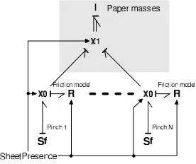
Modelling the transport of paper through the path involves three key elements: pinches, sheets and a friction model. These are shown in Figure 2.1. The energy to drive a sheet is delivered by the pinches1
. This energy is transported to the sheet and is influenced by the friction model.
Figure 2.1: Complete plant model
To explain the basics behind this model a simplified model is introduced in Figure 2.2(a). The pinch is replaced by a flow source, the paper by an I-element representing its mass and the friction model is contained in the R-element. From this figure it becomes clear that the driving force on the paper originates from the velocity difference (∆v) between the paper and the pinch.
1
This relation can be written as:
Fsheet=f(∆v) =f(vpinch−vsheet) (2.1)
Wheref(∆v) is the friction model function contained in R.f(∆v) can be of any form but within the limits set by the requirements.
Since a sheet is not continuously in a pinch, decoupling has to be added. This can be done by using a switching 0-junction (Mosterman and Breedveld, 1999). This results in the structure shown in Figure 2.2(b). The X0-junction sets the effort to the I- and Sf-element to 0 or to the effort coming from the friction model depending on the presence of a sheet.
(a) Coupling principle (b) Introduction of X0-junction for
decou-pling
Figure 2.2: Coupling of a pinch with a sheet
When adding pinches the question rises: “what to do when a sheet is in two pinches?” To answer this question as complete as possible would involve detailed measurements on the movement of the paper with respect to the pinches. Since the only sensors available to measure displacement are the encoders it is not possible to measure the behaviour of a sheet. Using more advanced measuring equipment (i.e. a high speed camera) a better friction model can be derived. This is future work since the friction model will be expendable as it is one of the requirements for the design.
An assumption is made on the behaviour of a sheet when pinched by two pinches. The assumption is that the pinch near the leading edge has more influence on the resulting force on the sheet than the one near the trailing edge. This assumption only holds when the leading edge pinch has an equal or higher velocity (vlead) than the trailing edge pinch(vtrail). When this
holds, the leading pinch will try to get the sheet at vlead while the trailing one tries to keep it
at vtrail. Due to slip and the higher velocity of the leading pinch the resulting velocity will be
nearvlead.
This means that the force from a pinch on a sheet can have three states. To implement this the model in Figure 2.2(b) is altered as well as the friction equation (2.1). The results are shown in Figure 2.3(a) and equation 2.2.
Since X0-junctions can only switch on or off it has been replaced by normal 0-junctions and the “switching” is moved to the adjustable R-elements. SheetPresence now gives a tristate output S:
• S = 0 when no sheet is present in the pinch
• S =Srear when the pinch is on the trailing edge of the sheet
• S =Sf ront when the pinch is on the leading edge of the sheet
WhereSrear and Sf ront are the fractions of the force applied to the paper. The force output of
an R-element is now given by:
Currently the friction model is implemented as:
F = ∆v
Ts
·msheet·S (2.3)
Where Ts is the sample time and msheet is the mass of a sheet. This means the F will be
calculated such that ∆v will be cancelled in one sample step. The fact that this is not a real friction model will be taken into account in the design of the control system.
To enable multiple sheets in the path, the model is extended (Fig. 2.3(b)) with a mul-tidimensional I-element, representing multiple sheets and a switching 1-junction introducing a mechanism for coupling one or two pinches to any sheet. Coupling is done with the same mechanism as for computing theS for the friction models.
(a) 1 sheet with 3 pinches (b) M sheets with 3 pinches (c) M sheets with N pinches
Figure 2.3: Bond graph representation of linking sheets with pinches
Figure 2.3(c) shows the layout of the model withN pinches added. The power bonds from the pinched are combined into a multi-dimensional bond for a better insight in the model structure. The friction models of all pinches are combined in one R-element.
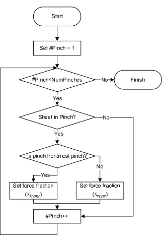
The presence of a sheet in a pinch follows from the position of the sheets. The“SheetPresence” computations are combined with the I-element and the X1-junction. Together, they form the “Sheet Intelligence” sub-model (Figure 2.1).
The main functionality of the “Sheet Intelligence” sub-model is shown in Figure 2.4. For each sheet in the system this loop is executed. The sheets position is compared to that of all pinches. When a pinch is in contact with a sheet, the role of that pinch (front or rear) is determined. Next to this loop, the positions of all sheets are compared to those of the the paper detectors, when a sheet is on top of a sensor, the value of that sensor is set high.
Figure 2.1 shows two inputs to the model, the PWM signal and a FeedSheet signal. The latter is used to tell the model to insert a new sheet into the system. This is done to eliminate the need for a model of the first pinch in the PIM. This pinch is driven with maximum acceleration to guarantee a better separation of the entering sheet from the other sheets in the tray. Due to this high acceleration the friction is even harder to predict. Since this does not influence the actual paper transport, this pinch is “modelled” as an extra input.
With all model parts explained the next section shows the results from various test performed to ensure the correct working of the model.
2.2
Verification and Validation
Figure 2.4: Flowchart of sheet intelligence sub-model
pinch model is proved in Appendix F. Hence, only the functioning of theSheet Intelligence and
Friction Model will be tested.
2.2.1 Verification
To verify the model, the pinches are set to rotate at a constant speed. The velocity of each pinch is higher than the previous. These speeds are chosen close to operation speed, 10,15,20 and 25 rev/s respectively. By setting the FeedSheet input high, one sheet is entered into the path and the following is checked:
• The logic functioning contained in the “Sheet Intelligence” sub-model.
• The dynamics, i.e. the force on the paper and its velocity.
• The paper flow visually, using a3D animation model.
• The ability to do real-time simulations.
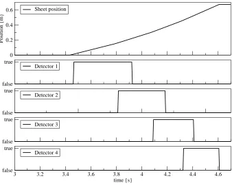
Logic functioning When the FeedSheet input is set high, a sheet should be transported through the path. The detectors should detect a sheet when it is on top of them. This proves that the logic functions in the “Sheet Intelligence” sub-model connect the energy from the correct pinch to the sheet. This can be observed in Figure 2.5. The position of the sheet increases with the time and the correct working of the detectors is shown as well.
Dynamics On each contact of a sheet with a pinch, the velocity difference is transformed into a force (2.2). The force should have a peak at the first moment of contact due to the friction model implementation (2.3). When a sheet is pinched by two pinches, there will be a constant velocity difference between the sheet and both pinches. This should be observable as a constant force on the pinches unequal to zero.
0
Figure 2.5: Model verification showing the correct transport of a sheet
the entering of the sheet in the first pinch. The following three peaks in the top graph show the entering of the sheet in the next three pinches. These peaks are smaller since the velocity difference is smaller. The forces on pinch 2 and 3 between the labels a and b
show what happens when the pinch on the leading edge of the sheet pulls the sheet faster that the rear end pinch allows. Pinch 3 has to pull extra hard to keep the sheet at the required velocity. and the force on pinch 2 is smaller due to the change of S to Srear in
the friction model(2.2).
3D animation model To verify the working of the model as a whole a 3D model has been designed (Figure 2.7) Animating this model with the simulation data enables a quick insight in the correct functioning of all components.
Real-time simulation To verify the real-time simulation requirement, code is generated from the model. This code is compiled and executed on the HIL simulator as described in Section 1.1.1. When executed, the target processor had idle time left. This proves the ability to simulate the model real-time.
Without further prove it is stated that the ability to generate code from the model is tested and found to be possible. Also the ability to simulate the model in real-time is checked, and found to be successful. The last requirement set in Chapter 1 is the ability to easily add a pinch. This is possible and is shown in Appendix G.
0
Figure 2.6: Forces on sheet and pinches
2.2.2 Validation
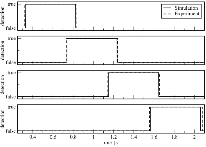
Comparing the modelled paper path with its real counterpart is done with a similar experiment as for verification. The motors are all set to rotate at 10 rev/s and one sheet is entered into the path. This results in the four paper detectors detecting the sheet sequentially. The comparison between the sensor signals from the simulation and the experiment is shown in Figure 2.8.
This figure shows that in the model the paper is detected for a shorter period than on the real plant. The reason for this is shown in Figure 2.9(a). The bundle of light emitted from the sensor has a width of 1 cm at the height the sheet passes. This results in a too early start of detection of the sheet as well as a too late end of detection. This results is a too long high time of the detector as shown in Figure 2.8. A solution to this problem is to confine the light by placing a small block with a hole in it on top of the sensor. The largest dimension of the sensor, its width, is 4 mm therefore this is the diameter of the hole. This is shown in Figure 2.9(b).
false true
detection
Simulation Experiment
false true
detection
false true
detection
0.4 0.6 0.8 1 1.2 1.4 1.6 1.8 2 time {s}
false true
detection
Figure 2.8: Comparison of detector signals between simulation and experiment
To verify the correctness of the solution presented above, a second experiment is performed with the same conditions as the first one but now with the blocks in place. Figure 2.10 shows the result of this experiment. In the left figure, the rising edges of detector 3 show that the detection of a sheet is closer to the simulated detection. The same holds for the falling edges shown in Figure 2.10(b).
Using only the paper detectors, the comparison between the model and real paper path can only be based on signals of detectors. Therefore it is not possible to comment on the correctness of the friction model other than that the detections of paper in simulation is so close to detections on the real plant that the plant model is at least close to reality on a global level. Hence, it is safe to conclude that a detailed friction model is not required in order to simulate the paper transport as required for controller design.
From the verification and validation results above it is concluded that the model satisfies the
(a) Sheet detector
without light bundle cofinement
(b) Sheet detector
with light bundle
cofinement
1.551 1.554 1.557 1.56 1.563 1.566 1.569 time {s}
false true
detection
Simulated With guide Without guide
(a) Rising edges of the third paper detector
2.055 2.058 2.061 2.064 2.067 2.07 2.073 2.076 2.079 2.082 2.085 2.088 time {s}
false true
detection
Simulated With guide Without guide
(b) Falling edges of the third paper detector
Figure 2.10: Comparison between simulation and experimental detector signals with and without bundle confinement
requirements set in Chapter 1 and can be used in stage 1, the model in-the-loop simulation.
2.3
Recommendation
Section 2.1 describes the replacement of the switching 0-junction with an extended R-element. From a functionality point of view, this is correct. However, from a model structure point of view this obscures the structure of the coupling between sheet and pinch. Adding a switching 0-junction and changing the R-element is a straightforward operation. Limitation in time pre-vented the implementation of this structure. An impression of the resulting model is shown in Figure 2.11.
In a printer, the printing of the image onto the paper is performed at the fuse. In the paperpath case the function of the fuse pinch is represented by the last pinch. A fuse rotates at a fixed speed and gets the images with a fixed time interval. This results in the following general control law requirement for a printer: Control the velocity of all pinches in the path previous to the fuse such that the sheets arrive at the fuse with a fixed velocity and a fixed distance between them.
This will be the goal for the controller described in this chapter. Besides the control law, this particular setup has a demonstration purpose, meaning that the transport of paper through the path has to be visually attractive. These two requirements form the basis of the control concept described in Section 3.1.
Next, the control system is split up into three subsystems each with a specific task. This presented in Section 3.2.
In Section 3.3 the functionality is verified with simulations and validated using the paperpath setup.
3.1
The control concept
Transporting a sheet through the paper path with a known arrival time (tf use) requires a
prede-termined velocity profile. To make the paper path behave like the printer referred to in Chapter 1, two features of this printer are incorporated, alignment and velocity correction. To let an alignment mechanism act on a sheet, it is stopped for a fixed amount of time (van Kampen, 2003). This is applied in the velocity profile of pinch 2. The third pinch is used to accelerate the paper to ensure the correct arrival time at the fuse. When reaching the fuse, the paper should have a fixed and stable velocity. Therefore the paper should be decelerated to the fuse velocity before it reaches the fuse. Taking the settling time of the pinch velocities (Appendix F) into account when determining the moment of deceleration, a stable velocity at the fuse can be guaranteed. To ensure the paper is firmly thrown out into the collection bin the fourth pinch accelerates the sheet just before it leaves the path.
The full profile has the form as shown in Figure 3.1. The variables in this figure are declared in table 3.1. All time variables are given with reference to t0 = 0[s]. The numbered surfaces
represent the pinches that pinch a sheet. The shaded areas are three locations where a sheet is pinched by two pinches. To eliminate control problems due to friction, the acceleration and deceleration actions are only performed when a sheet is in one pinch. Since the paper detectors are placed just after each pinch, acting after a falling edge of the detector of the trailing pinch realises this. The equations for computing the profile shape are discussed in Appendix A.1.
tpim Sheet reaches the first paper detector Measured
talign,1 Sheet leaves first paper detector Measured
Start of the alignment profile
talign,2 End of the stand still for alignment =talign,1+ ∆tstop
∆tstop Required time for alignment Parameter
tcorr,1 Sheet reaches third paper detector Measured
Start of the velocity correction profile
tcorr,2 End of the velocity correction profile Computed (A.3)
∆tdecel Time needed to decelerate fromvcorr to vf use Computed (A.7)
tf use Sheet reaches last paper detector Computed (A.1)
vf use Required sheet velocity at the fuse Parameter
vcorr Velocity required to get paper at the fuse attf use Computed (A.5)
vmax Maximum velocity allowed in the path Parameter
Table 3.1: Explanation of variables from figure 3.1
With the velocity profile for a sheet given, the separate profiles for the pinches can be extracted. Below the actions taken upon edges of the detector signals as shown in Figure 3.1 are listed. These are the key action in the system and will form the basis of the control system layout described in the next section.
Rising edge P DP IM: Computetf use (A.1)
Falling edge P DP IM: Start alignment profile on pinch 2
1. Decelerate to 0m/s
2. Keep at 0m/s for ∆tstop seconds
3. Accelerate tovf use
Falling edge P Dalign: Start correction profile on pinch 3
1. Compute vcorr (A.5)
2. Accelerate tovcorr
3. Keep at vcorr untilt=tcorr,2−∆tdecel
4. Decelerate to vf use
Falling edge P Dcorr: Start the throwout profile on pinch 4
1. Keep at vf useuntil 5 cm of paper is left in the pinch
2. Accelerate tovmax
Falling edge P Df use: Stop the throwout profile
To structure the control system and support the distribution requirement, the actions de-scribed above are separated into different sub-systems.
3.2
The control system layout
• Supervisory Controller
– Detection of edges in paper detector signals
– Computetf use
– Computevcorr
– Start and stop profiles
• Sequence Controllers
– Execute the profiles started by the supervisor
– Compute the references to be send to the loop controllers
• Loop Controllers
– Keep the motors velocity at the reference received from the sequence controller
– Contains the control algorithm (i.e. PID)
Each pinch has its own sequence controller and loop controller. In Appendix B a more detailed description will be given on the three controller parts. The design of the loop control is treated in Appendix F.
Figure 3.2: Control system overview
3.3
Verification and validation
To verify the correct working of the control system, the complete system is simulated feeding one sheet through the path. This sheet should follow a reference profile similar to that in Figure 3.1 and should arrive at the fuse on the correct time. Figure 3.3 shows the simulated velocity profile of a sheet together with the detector signals. This simulation shows is that the control structure works and implements the proposed velocity profile correctly. The maximum velocity set for this simulation is 2 m/s. As the top graph shows, this velocity is not reached. The maximum acceleration prevents reaching this velocity before the sheet is out of the pinch.
To check the correct working when feeding more than one sheet through the system, a new simulation is performed. In this simulation 50 sheets are fed through the system at 50 pages / minute. This resulted in Figure 3.4 showing that each sheet arrives at the fuse at the correct time. Figure 3.5 shows the resulting error graph when transporting 50 sheets at 100 pages / minute. The errors shown in both figures are the result of rounding errors. The two results lead to the conclusion thet the control systems functions as expected.
0 0.4 0.8 1.2 1.6
velocity {m/s}
Sheet velocity
0 0.5 1 1.5 2 2.5 3
time {s} false
true
Detector 1 Detector 2 Detector 3 Detector 4
Figure 3.3: Verification of the sheet velocity profile
0 10 20 30 40 50
Page {#} 0
2e-15 4e-15 6e-15 8e-15
Time {s}
Arrival Error
Figure 3.4: Arrival error of 50 pages at 50 pages/minute
0 10 20 30 40 50
Page {#} 0
1e-15 2e-15 3e-15 4e-15
Time {s}
Arrival Error
In the previous chapters a model and a control system have been designed. The next step in the design approach described in Chapter 1 is the embedded control system implementation. One of the goals of this project is the design of a distributed control system. In Chapter 3, the description of the control system does not include the distribution. Therefore this has to be designed first. Section 4.1 describes this design. In the following section the route from design tool to embedded target is described. This chapter concludes with a simulation and experiments proving the correct working of the described system.
4.1
Distributed control implementation
The decomposition of the control system intofunctional blocks is described in Section 3.2. The next step is to separate these blocks, such that each subsystem (supervisor, sequence controller, loop controller, paper detector) can be deployed to a different target1
. To support the evaluation of different distributions, this separation has to be as extensive as possible. The distribution as shown in Figure 4.1 supports this principle.
Figure 4.1: Overview of the sub-system split-up
All functional blocks are now separated into subsystems. With an appropriate communica-tion bus between different targets, it is now possible to put each subsystem on a different target. Grouping subsystems together on one target is also possible. By adding a communication bus, a delay is introduced. This should be compensated for in the control algorithms.
4.1.1 CAN bus delay
An earlier study (Groothuis, 2004) showed the correct functioning of the CAN bus in combina-tion with the PC104 targets. Furthermore synchronisacombina-tion of the targets has been established (Huang, 2006). The worst case delay introduced by the CAN bus has been measured (Groothuis, 2004) using the same hardware as for the paper path setup. It was shown that the worst case transfer time was 250µs. Figure 4.2 shows that if the duration of the read and write process during the execution of the main software loop do not exceed 750µs, the CAN message will be at the receiving end before the next “read”. Therefore, the CAN bus is modelled as a delay of one sampling interval.
1
Figure 4.2: Transfer of a CAN message
4.1.2 Controller distribution
In (Otto, 2005) a number of distributions was discussed. One of them is chosen as the test example for this project. This distribution is shown in Figure 4.3.
Figure 4.3: Overview of the chosen distribution
The figure shows three nodes connected to the plant and one supervisor node. The paper detectors are combined with the sequence and loop controller of their respective pinches. The node they are connected to takes care of sending the signals over the CAN bus to the supervisor. Furthermore, the loop controllers are implemented on the same node as their respective sequence controllers.
In a real printer, the input module as well as the finisher are not a fixed part of the printer. They are easily replaceable. The distribution chosen here resembles this principle. The input module and finisher at node 1 and 3 respectively can easily be replaced.
In this distribution the reaction of a sequence controller to an edge of a detector signal is delayed by Ts = 1[ms] because it has to be send to the supervisor first. The delay affects all
Figure 3.1 shows the distance to travel during the correction profile, x3 = 9[cm]. When the
detector signal arrives two sample intervals too late, x3 becomes x3 = 0.09−2·Ts·vf use[m].
This new value of x3 is used in A.5 to computevcorr.
The control system shown in Figure 4.3 can be used in a centralised control approach. This eliminates the CAN bus and therefore the delays. Hence, the control algorithms need to be adjusted.
4.2
From design tool to embedded target
The last step is to get the controller from a 20-Sim model to an executable on the target system(s). The part of the 20-Sim code template that handles the coupling between the control system and the CAN bus has not been finished yet. Hence, only the centralised controller has been implemented on the target.
Figure 4.4: ForSee toolchain overview
Figure 4.4 shows an overview of the ForSee toolchain (Visser, 2007; Buit, 2005; Posthumus, 2006). This toolchain is used for the transfer of the control system to the target hardware.
First c-code is generated from the 20-Sim model. In the target connector, the inputs and outputs of the control system are connected to the correct I/O pins on the FPGA board. Next the code is compiled and deployed to the PC104 target hardware. The toolchain facilitates logging of all variables in the control system. This is used to get the measurement data for the validation experiments.
4.3
Simulations and experiments
With the executable for centralised control generated, experiments are performed to verify the correct working of the control system on a PC104 target.
4.3.1 Centralised control experiment
Experiments performed on the real setup as described in Appendix C show that the system works correctly.
These Experiments show that when removing the extra beam guides on the paper detectors the correct arrival fails. This is due to the fact that the supervisor reacts on the edges of the detectors assuming they detect the sheet when it is exactly at the centre of the detector. Therefore, the guides are a good addition to the setup.
Another critical part in the paper path is the “Paper Input Module”. Slip at the first pinch prevents the sheet from entering the path on the time expected by the controller. This holds for real printers. Making the first pinch accelerate with an acceleration near infinity solves part of this problem, but does not prevent all sheets from arriving late at P DP IM and therefore at the
fuse.
4.3.2 Distributed control simulation
In Section 4.1.1 it was stated that the delay of a CAN message can be modelled as a delay of one sampling interval. To verify if the control system can handle this delay, a simulation is done in which all CAN messages arrive with one sampling interval delay.
Figure 4.5 shows two arrival comparisons. Graph (2) shows that the arrival actually gets worse when the computation ofvcorr is compensated for the delay. Graph (3) shows that when
removing the delay compensation, the arrival of a sheet with and without the CAN delay are much closer. The remaining difference is due to the rounding of variables in the model. The reason for the better working of the control system without compensation is that all signals involved in the control of the sheet velocity are delayed and the supervisory algorithm already compensates for that. When delaying the signal from P Dalign one sample interval more (e.g. 2
intervals in total), the need for compensation does arise and proves to work. This is shown in graph(4).
2.282 2.2825 2.283 2.2835 2.284 2.2845 time {s}
0 1
PD fuse value {}
No Delay (1)
1 ms delay, compensated (2) 1 ms delay, not compensated (3) 2 ms delay, compensated (4)
5.1
Conclusions
Stage 1, model in-the-loop simulation, of the design trajectory (Visser and Broenink, 2006) has been completed. The two parts required, a model of the plant and a control system, have been designed and tested.
The model proved to satisfy all the requirements. In Chapter 2 the code generation was ver-ified and simulation results show that simulation can be performed in real-time (HIL simulation is possible). The easy addition of pinches has been shown as well (Appendix G). The friction model could not be verified but proved not to be a problem when using the model for control system design.
The controller was designed and simulated as a centralised controller in Chapter 3. It was shown that the control concept works in simulation. In Chapter 4 the concept of the distribution was explained and implemented in the control model. The proper functioning of the centralised controller was shown. Distributed control could be tested in simulation only, and proved correct. By showing that the controller is able to work on the embedded control system, it was proved that the designed control system is suitable for code generation.
As an improvement of the results of the control system, light beam guidance was suggested and implemented. Experiments showed this was of vital importance for the performance of the control system.
5.2
Recommendations
Evaluate design trajectory Stage 1, model in-the-loop simulation, has been completed. Us-ing the developed model and control system the steps 2 through 6 of the design trajectory should be carried out and evaluated.
Distribution of the control system Since the software for inter-node communication was not ready, this has not been tested. Once the software has been completed, the implemen-tation of the distributed control system is straightforward.
Improvements on setup and software
• Position measurement
By adding an improved position measurement, two problems can be solved:
1. To obtain a good friction model, the actual position of a sheet has to be measured continuously. This can be done i.e. by using a high speed camera. This measurement solution is expensive and should only be used once to determine the friction between paper and pinch.
2. Improving the accuracy of the paper detectors requires a cheaper measurement solu-tion. As a first attempt to get more accurate results without extra costs, the sensors could be placed closer to the sheet. That way the remaining beam width error (2.5 mm) can be solved. Next to that, the measurement speed could be increased. This can be done i.e. by connecting all paper detectors to one embedded control system and let that node run at a higher sampling frequency. A form of estimation could also be used to obtain more accuracy.
• Improvement of the control system
Two features have not yet been included in the control system.
2. A safety layer. When sheets collide or get stuck in a pinch the operator now has to manually press an emergency button while this event can easily be detected using paper detector information.
• Improvement of the paper path setup
This appendix describes the calculation used to get the velocity profile as depicted in A.1. Table A.1 describes the parameters and variables used for the computations.
A.1
Sheet velocity profile
Figure A.1: Overview of the sheet velocity profile
tpim Sheet reaches the first paper detector Measured
talign,1 Sheet leaves first paper detector Measured
Start of the alignment profile
talign,2 End of the stand still for alignment =talign,1+ ∆tstop
∆tstop Required time for alignment Parameter
tcorr,1 Sheet reaches third paper detector Measured
Start of the velocity correction profile
tcorr,2 End of the velocity correction profile Computed (A.3)
∆tdecel Time needed to decelerate fromvcorr to vf use Computed (A.7)
tf use Sheet reaches last paper detector Computed (A.1)
vf use Required sheet velocity at the fuse Parameter
vcorr Velocity required to get paper at the fuse attf use Computed (A.5)
vmax Maximum velocity allowed in the path Parameter
Table A.1: Explanation of variables from figure 3.1
First step is to compute the required arrival timetf use(n) for the nth sheet.
tf use(n) =tpim(1) +
xtotal
vf use
+ ∆tf use·n (A.1)
∆tf use=
xintersheet
vf use
(A.2)
Withn the number of the sheet, tpim(1) the insertion time of the first sheet of the “print job”,
xtotal the length of the path the sheet has to travel andxintersheet the required distance between
the sheets on arrival at the fuse.
When the sheet has left the align pinch, the real value of tcorr,1 is known and the last part
the velocity to stabilise (tdamp) and is therefore defined as:
tcorr,2=tf use−tdamp (A.3)
This leaves vcorr to be calculated as the velocity required reach the fuse at tf use. This can be
written as the distance to be travelledx3.
x3 =vf use(tf use−tcorr,2) + (vcorr−vf use)(tcorr,2−tcorr,1)−
(vcorr−vf use)2
amax
(A.4)
With amax the maximum acceleration, a system parameter. Solving (A.4) for vcorr yields the
equation for the required velocity:
vcorr=−
1
2t3amax+vf use+
1
2tcorr,2amax− (A.5)
−12pamax(tcorr,12amax−4tcorr,1vf use−2tcorr,1amaxtcorr,2+tcorr,22amax+ 4vf usetf use−4x3)
This velocity has two boundaries:
0≤vcorr ≤vmax[m/s] (A.6)
The lower boundary is set to 0 because when the sheet travels backwards, the system is unable to keep track of it.
To determine when the sheets velocity should be brought back to vf use, the time required
for deceleration needs to be found. This time is taken as the time it takes to get formvcorr to
vf use with maximum accelerationamax:
∆tdecel=
vcorr−vf use
amax
This appendix describes the controller parts as mentioned in Section 3.2 in detail.
B.1
Supervisor
Before “printing” can start, the supervisor receives four parameters from the user. These are the number of pages per minute to transport (ppm), the inter-sheet distance they should have (isd), the number of pages to process (N) and the time required for alignment (tstop). With
these parameters and the signals from the paper detectors the supervisory controller performs the following tasks:
Discover edges on the detector signals Each time the supervisory control loop is executed, the current value of the detector outputs is compared against the previous ones to deter-mine if there has been a change. When an edge occurs the required action is taken.
Record tf irst When the first sheet of a job enters the path, a rising edge is detected onP DP IM.
The time is now recorded for use in calculating the required arrival times.
Compute tf use(n) Every sheet entering the path induces a rising edge of P DP IM. The
re-quired arrival time of the nth sheet (t
f use(n)) is now computed as tf irst plus the time
required to travel the path length plus n over ppm for the interval at which each sheet should exit the path in order to reach the required number of pages per minute.
Start alignment profile When a sheet leaves the first pinch, a falling edge ofP DP IM occurs.
A signal is sent to the responsible sequence controller that starts the alignment profile.
Start correction profile When a sheet leaves the second pinch, a falling edge ofP Dcorroccurs.
Now the required correction velocity (vcorr) is computed (A.5). Thevcorr signal is sent to
the responsible sequence controller together with a start signal.
Start throwout profile When the sheet leaves the third pinch a falling edge ofP Dalignoccurs.
A signal is now send to the responsible sequence controller to start the throw out profile.
B.2
Sequence controllers
Each sequence controller is responsible for its own part of the profile shown in Figure 3.1. They compute their reference outputs with the signals coming from the supervisor as described above and seven extra parameters, shown in table B.1. These parameters are sent to the sequence controllers before the start of a “print job”.
Name Description Parameter type
vmax Maximum velocity System parameter
amax Maximum Acceleration System parameter
SheetW idth Width of the paper used System parameter
isd Inter sheet distance Job parameter
ppm Required pages per minute Job parameter
N Number of sheets to process Job parameter
tstop Required alignment time Job parameter
Due to lack of resolution in measuring the velocity of the motors, the position is used in the loop controllers (See Appendix F). With the position as controlled variable, also the reference has to be a position. This is achieved by integrating the reference velocity profile.
Appendix A discusses the computation of the reference profiles in detail.
B.3
Loop controllers
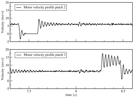
This appendix is an addition to Section 4.3.1. It describes the experiments to verify the correct working of the control system on the real setup.
To check the correct working of the controller after implementation on the embedded control system an experiment is carried out to compare the results from simulation with those from the setup. Since only the sheet detectors on the setup can be used to measure the behaviour of a sheet of paper, only those are compared. The correctness of the alignment and correction parts of the profile can only be derived out of the correctness of the arrival time at the fuse. However, the stopping and speeding up of a sheet can be deducted from the motor velocities as well. The two figures below show these features. Figure C.1 shows the arrival time error of 20 sheets and Figure C.2 shows the actual stopping and speeding up of the alignment and correction pinch respectively.
10 20
Time {s} -0.015
-0.01 -0.005 0 0.005 0.01 0.015 0.02
Time {s}
Arrival Error
Figure C.1: Arrival error of 20 pages at 50 pages/minute
The arrival of the sheets is not as accurate as seen in the simulation results. Two types of errors are seen, negative and positive values. The negative error means the sheet arrives too early at the fuse. The main reason for this has already been explained in Section 2.2.2. The width of the paper detector detection area is such that the detection of the arrival of a sheet is too early. In this experiment, a sheet travels at about 0.25m/s, with an error of 0.01s gives a early detection distance of 2.5mm. This is exactly half the width of the beam after placing the confinement (Figure 2.9(b)).
-5 0 5 10 15 20
Velocity {rev/s}
Motor velocity profile pinch 2
7.5 8 8.5
time {s} -5
0 5 10 15 20
Velocity {rev/s}
Motor velocity profile pinch 3
The image shown below depicts the design trajectory as developed in (Visser and Broenink, 2006).
Plant parameters
H-bridge voltage 25[V]
Pinch radius 13.9[mm]
Position Pinch1
1 0.00[m] Position Pinch 2 0.145[m] Position Pinch 3 0.320[m] Position Pinch 4 0.495[m]
Position Sheet Detector 1 0.012[m] Position Sheet Detector 2 0.186[m] Position Sheet Detector 3 0.361[m] Position Sheet Detector 4 0.537[m]
Name Pinch 1 PIM pinch Name Pinch 2 Alignment pinch Name Pinch 3 Correction Pinch Name Pinch 4 Fuse / finisher pinch
Encoder counts / revolution 2000
Cogs motor wheel 18 Cogs Pinch wheel 37 Cogs Teeth Belt 90
Table E.1: Parameters of the paper-path setup
Notes:
1. All pinch and detector positions are measured with reference to pinch 1.
System Requirements
Table E.2 shows the requirements set for this project. The values are generalised from values suggested by the participants of the BodeRC project.
Transport volume 100[pages/minute] Space between pages 50[mm]
Page width (A4) 21.0[cm] Max. paper velocity 2[m/s] Max. paper acceleration 20.0[m/s2
]
Max. motor speed 47[rev/s] Max. motor acceleration 470[rev/s2
]
Control parameters
Table E.3 shows theJob parameters that can be set for each print job.
Description Name in model Typical value Inter sheet distance ISD 50 mm Pages per minute ppm 50 ppm
Number of pages N 50
Alignment time AlignTime 200 ms
The goal of modelling the pinch is to get insight into the dominant dynamical behaviour. This insight is used to design the loop controller. The extend to which details of the system are modelled depends on their influence on the controller design. The model has to be accurate enough to enable good controller design. Determining the necessary accuracy is an iterative process of which the result will be presented here. Two questions have to be answered in this chapter:
1. Is the model accurate enough?
2. Can the final loop controller meet the requirements?
In this chapter first the modelling of the pinch dynamics is treated. After the model has been developed, it is verified with simulations and validated with experiments on the real setup. With the model a controller is designed, as is described in Section F.3. Combining the model and the controller simulations are done to check if they behave as expected. These simulations and their results are described in Section F.4.1. When the behaviour of the pinch and controller model are satisfactory, experiments on the real setup can be performed. These experiments are treated in Section F.4.2. At the end of this chapter concluding remarks are made on the design model and controller.
F.1
Modelling
Looking at the setup shown in Figure F.1, the pinch can be seen as three different parts: 1. The driving part(motor, and h-bridge)
2. The driven part(pinch inertia, frictions) 3. The coupling part(belt and pulleys)
Figure F.1: One of the pinches in the paper-path setup
As shown in figure F.2 the driving and driven part can be found left and right from the “BeltDisturbance and Gear” sub-model. This third part takes care of the transmission as well
as the disturbance introduced by the transmission.
Figure F.2: General model of a pinch in the paper path
possible. Therefore the simple dc-motor model depicted in Figure F.3 is used.
Figure F.3: Simple DC-Motor Model
In this model, the current is calculated from the input voltage and the internal states (speed and current). The motor torque is calculated from the current added with a friction component. The main friction in the motor is coulomb friction, therefore this is the only friction included in the model. The coulomb friction is speed and direction dependent. The motor specifications can be found in its data sheet (MaxonRE25, 2006). A complete list of parameters used in the sub-model can be found in Table F.1.
Terminal Inductance L 0.238 mH
Terminal Resistance R 2.19 Ω Torque Constant1
K 23.4 mN m/A
Rotor Inertia J 10.7 kgm2
/rad
Coulomb Friction Tc 0.8118 mN m
Table F.1: Motor model parameters
Next to the motor model the driving part of the model includes a representation of the H-bridge used in the real setup. In the model the “H Bridge” is a multiplication of the percentage
1
pulse width modulation(PWM) times the h-bridge voltage. The block “Rad2Rev” is used to convert the motor speed reading in [rad/s] to [rev/s]. This measurement is used in the feedback loop of the controlled system.
The coupling sub-model (Figure F.4) holds two functions. The first one is the gear with timing belt that is placed between the motor shaft and the pinch shaft. The “BeltDisturbance” block represents an effect that was observed during experiments with the real system. Velocity measurements showed that there was a sine like disturbance. The frequency of the disturbance turned out to be linearly related to the speed of the motor times the ratio between the tooth on the timing belt and the tooth on the largest pulley.
fdisturb[Hz] =ωmotor[rev/s]×
37
90 (F.1)
The function that is used for the simulation of this effect is a squared sine wave with a small amplitude that has to be tuned to the disturbance observed in the real setup. It has a frequency of 1
2·fdisturbsince squaring a sine wave doubles its frequency. After experiments with
the real setup it was concluded that the fast changing velocities did not have effect on the belt disturbance, only a disturbance related to the mean velocity was observed. Therefore the filter block is included to reduce the effect of fast changing velocities.
p1
Figure F.4: Sub-model with belt-disturbance and gear
Figure F.5: Model of the pinch mechanics
At the right side of Figure F.2 the sub-model of the pinch mechanics is shown. The contents of that are presented in Figure F.5. Two sorts of friction are distinguished here, viscous friction and coulomb friction. For both frictions the parameters are not known beforehand and have to be estimated2
. From experiments it showed that a combination of d= 250[µN ms/rad] for the viscous friction and Fn= 2.2[mN] for the coulomb friction yields a correct behaviour of the
pinch in open loop. Experiments that show the correctness of these values will be presented in Section F.2. The other element in the pinch model is the inertia of the pinch itself. This inertia represents all of the rotating parts at the pinch side of the system, including an iron rod, four rubber wheels and the pulley. Since the mass of the iron rod is by far the dominant one, all
2
Experiments on the influence of friction in this kind of systems performed by Oc´eshow that the influence of
other masses are neglected and the inertia Jpinch is calculated from the mass and radius of the
rod alone as shown in equation F.2, where m is the mass of the rod and r its radius. Exact values will be calculated in Section F.2.
Jpinch =
In the bottom right part of Figure F.2, a belt-pulley combination is included. This combi-nation transforms the rotation energy of the pinch to the translation energy of the paper. This element is used to connect the pinch model to the plant model as described in Chapter 2.
The mass of the paper itself is not included since it is too small to have a noticeable effect on the dynamic behaviour of the system in our region of interest. However, the presence of paper in the system does have influence on the dynamics of the system due to stick and slip effects as shown in (van Kampen, 2003). This behaviour will be modelled outside the pinch model and will therefore be treated in Chapter 2.
F.2
Model Verification and Validation
In order to check whether the model described in the previous section behaves as expected first simulations are done with 20-Sim. These simulations are used to check for strange behaviour and to adjust parameters such that the response is as expected. When the model behaves like expected the simulation results are compared with results obtained from the real setup. With this comparison remarks can be made on the validity of the model.
F.2.1 Verification
After finishing the model, the first simulation that shows how the model behaves is an open loop test. This is done by just applying a step input to the PWM input of the model and recording the output. The result of the first simulation is plotted in Figure F.6.
0
Figure F.6: Open loop simulation of the pinch model
As can be seen in the figure, the up and down ramping parts of the input have a slope that represents the maximum required acceleration and deceleration: amax= 470[rev/s2] and that the
maximum is such that the resulting motor speed is the required maximum: ωmax = 47[rev/s].
The position measurement, which can be acquired much more accurately, is used to validate the model.
From Figure F.6 it can be concluded that the model does not show unexpected behaviour and is capable of meeting the requirements as stated in Section E. To be able to draw more useful conclusions, next the simulation results will be compared with measurement data from the real setup.
F.2.2 Validation
To check whether the model represents the system close enough to facilitate good control design two experiments are performed. To perform a basic check to ensure the response of the real pinches is close to that of the model, the real pinch is excited with the same signal as in Figure F.6. We define the model accurate enough for controller design when the simulated position is within 10% of the measured one.
During the second test a sinusoidal input signal is applied of which the frequency is swept up to half the sampling frequency. The result of this experiment tells whether the frequency response is the same for the model and the physical system. The frequency response of the model is important since it tells whether the important dynamics of the pinch are represented well enough by the model.
Figure F.7 shows the result of the first test applied on one pinch. As can be observed from this figure the model behaves similar to the plant. The final angle of the real motor shaft and that of the model are slightly different due to imperfection in the estimation of the viscous friction parameter. Due to the coulomb friction component, the slopes of the motor angle measurement and simulation differ. It is possible to adjust the parameters but that would then have to be done for each pinch separately. Figures F.8 a and b show these differences for each pinch in the system. Both sub-figures show that the differences between the simulated and the measured angular displacement are well below 10% for most pinches and close to, but still below this percentage for the 1st pinch. Therefore from this analysis it can already be concluded that the
model is suitable for controller design and simulation. But to be sure the conclusion holds over the entire used frequency range the second test has to be done as well.
To measure the frequency response of the pinches and the model, they are excited with a sine with sweeping frequency from 0 up to 500Hz. The upper limit of 500Hz is chosen since the sampling frequency of the system is 1kHz as will be explained in Section F.3.1. The sweep is done in 100sec. This results in a frequency response plot for each pinch and the model, as shown in Figure F.9.
Two of the curves in Figure F.9 attract the attention as they differ significantly from the other four. These are the frequency response of the model and that of the 1st pinch. The
model response differs from the rest of the pinches again due to the imperfection in the friction parameter estimation. What’s more important than the height of the curve is its shape. The shape of the model response curve shows a good similarity with that of the pinches. This leads to the conclusion that the pinches do not show behaviour that is not modelled.
The differing response of the 1stpinch is due the fact that its mechanical configuration differs
slightly from the other pinches. Details can be found in (Otto, 2005). Since the first pinch is only used to insert paper into the system and not to control the behaviour of the paper it is considered noncritical. This means that no special adaptations have to be made as long as the pinch proves to be controllable. Controllability will be verified in Section F.3.
0
Figure F.7: Open loop comparison of the model and a pinch
controllers for the pinches themselves will be treated, in Chapter 2 the higher control layers (sequence and supervising control) will be treated.
F.3
Control Design
The angle of the motor needs to be controlled in such a manner that the paper sheet that is in the pinch follows a given reference profile. The velocity and acceleration requirements for this profile were already stated in the Requirements section (E). As a measure for good control it is stated that: “The position of the sheet has to be within a certain error margin from the desired position profile before it reaches the next pinch.” To make sure that this is achieved in the real system, the distance between two pinches used for controller design is taken smaller than in reality: dpinch= 10[cm].
To achieve the goal of following a velocity reference profile with the use of position control, the velocity profile is integrated to a position profile before it is fed to the input of the control system.
Controlling a position that has to follow a prior known profile can be done in two ways, through feed-forward or feedback. These two methods can be combined. A simple feedback controllers is a PID controller. If this controller can fulfil the task stated above then there is no need for more complex feedback or feedforward controllers. This will be investigated in Section F.3.1.
Since the profile to be followed is known beforehand, feed-forward can be used to make the system react faster on changes at the input. As the model developed in Section F.1 is not completely accurate and the parameters for each pinch differ it is decided that learning feed-forward suits our need best. In learning feed-feed-forward, the parameters of the algorithm can be learnt during operation, in a pre-operation learning period or a combination of both.
learn-0 0.5 1 1.5 2 2.5 3
(b) Comparison of the Final Angle
Figure F.8: Details of comparison between the pinch model and the measured angles
ing feed-forward method is investigated. Others methods that can be used are presented in de Vries et al. (2000).
F.3.1 Feedback: PID
The main reason for choosing PID control as feedback control is simplicity and a low number of computations needed. Since one of the goals of this project is to keep the software as simple as possible, it pays to investigate PID control. A short treatment of PID control in computer controlled systems is given in (Astrom and Wittenmark, 1997).
The initial control system (Otto, 2005), was based on velocity control at a sample frequency of 100Hz. As shown in the work of Otto, the results were not satisfying. From experiment results it was concluded that the velocity measurement is not accurate enough. The position measurement showed to be much more accurate, therefore this will be used from now on to control the pinch.
In (Astrom and Wittenmark, 1997) a tuning method based on simulations and/or experi-ments is treated, the Ziegler-Nichols method. Since one of the key eleexperi-ments in the Controller
System Design Trajectory (Visser and Broenink, 2006) is the design of the control based on a
model of the process this method is suited for the design trajectory. Parameter tuning with the Ziegler-Nichols method starts with controlling the plant model with only proportional control. By setting the proportional gain such that the system just starts oscillating the value kp,border
is determined. Next the oscillation period (Tborder) needs to be determined. With these two
parameters, the three PID parameters (kp, τi andτd) can be computed as follows.
kp= 0.6×kp,border
τi = Tborder2
τd= Tborder8
(F.3)
1 10 100 frequency {Hz}
0 5000 10000 15000 20000
magnitude
Simulated Model Pinch 1 Pinch 2 etc.
Figure F.9: Frequency response of all five pinches
F.3.2 Feed-forward: MRAS-based Learning Feed-forward
A short investigation in this method did not lead to more accuracy of the control system. In Section F.4.1 it will be shown that a faster reaction on changes in the reference is not needed as well. Therefore it is decided that feed-forward will not be used in the control of pinches.
F.4
Controlled System Simulation and Experiments
Simulating the controlled system in order to tune the control parameters such that the controller can be used in practise without retuning requires extra modelling blocks to be added to the average simulation model. All the key features of the real control system running on an embedded pc and hooked up to the physical system have to be included. In Figure F.10 all these parts are shown. Obviously the controller and the plant are present, but the block between them are those blocks the represent features of the hardware in the embedded system.
Figure F.10: Top Level Simulation Model of one pinch
one time-step later than the input it is computed from. After the delay, the digital signal from the controller is converted to an analogue signal that is fed to the motor. In the physical system this is done in the H-bridge. In the return path of the control loop, starting from the pinch, firstly the “Encoder” is included. This block represents the real encoder mounted on the back of the motors. The “Sample” block represents the sampler present in the FPGA.
Now the simulation model is clarified, the simulations and experiments can be presented.
F.4.1 PID, simulations
Figure F.11 shows the model of the loop controller.
Figure F.11: Loop Controller model
The results of the control system for the pinches designed by (Otto, 2005) show that the ripple as discussed in F.1 is not suppressed by the controller. Tests with position control still show that the ripple is hard to remove from the output. By controlling the pinches at a sampling frequency of 1000Hz it turned out that the ripple, although still there could be tamed much further. Therefore, the sampling frequency of the control system is set to 1000Hz.
To tune the PID controller in simulation the Ziegler-Nichols method as described in Section F.3.1 is applied. The system just started oscillating with kp,border = 4.5.Taking the FFT of
the resulting angular error (Figure F.12) showed that the oscillation frequency lies at 1
Tborder =
45.6[Hz]. Applying Equations F.3 results in the PID-parameters as shown in Table F.2.
kp 2.7
τi 10.73·10−3
τd 2.68·10−3
Table F.2: Ziegler Nichols tuning results
Entering the values of Table F.2 into the PID controller, the system can be simulated. To test if the system will work properly at the maximum acceleration, this value ( ˙ωmax = 470[rad·s−2])
is used to compute the input profile. The acceleration is stopped at the maximum speed,
ω = 47[rad·s−1]. The results can be observed in Figure F.13. This figure shows that the controller is capable of making the pinch follow the given reference profile.
To ensure that the control requirement stated at the introduction of this section3
is met, the paper position is plotted against the paper position error using the same settings as in the first experiment. This plot is shown in Figure F.14 and shows that the paper position error reaches zero already before it is transported for 3[cm] by the current pinch. Since it was stated
3
0.5