R E S E A R C H
Open Access
Target scattering estimation in clutter with
polarization optimization
Xu Cheng
*, Longfei Shi, Yuliang Chang, Yongzhen Li and Xuesong Wang
Abstract
In this paper, we propose an adaptive waveform polarization method for the estimation of target scattering matrix in the presence of clutter. The proposed sequential algorithm, based on the concept of sequential minimum mean square error (MSE) estimation, to determine the coefficients of the scattering matrix, guarantees the convergence and the resulting computational complexity is linear with the number of iterations. The effectiveness of the proposed method is validated through numerical results, underlining the performance improvement given by joint transmission and reception (Tx/Rx) polarization optimization for the scalar system. Also, the results show that the vector system with transmission polarization optimization provides a comparative performance as the scalar measurement system employing joint Tx/Rx polarization optimization. Less computation burden highlights the advantage of the former mode.
Keywords:Radar polarization, Minimum MSE estimation, Sequential algorithm, Waveform design, Scattering matrix
1 Introduction
Polarization, together with the amplitude, time, fre-quency, phase, and bearing descriptor of radar signals,
completes the information description of target
returns from radars. The exploitation of information on the echo polarization can provide a significant improvement on radar performance [1]. To obtain the target polarimetric scattering information, conven-tional polarimetric radar systems alternately switch (or simultaneously transmit) the horizontal (H) and vertical (V) polarizations at the transmission side, and
simultaneously receive both polarizations at the
reception side, consequently resulting in four
polarization combinations: HH, HV, VH, and VV polarizations.
Motivated in part by recent advances in the hardware and sensor information processing, such as solid state transmission and digital arbitrary waveform generators, in modern radar systems, any polarization on either transmission or reception can be synthesized by using the linear combination of the H and V components.
Thus, besides the four types of transmitter/receiver combinations above, polarimetric radar can achieve any pair of transmitter/receiver polarizations. Such flexibility greatly enhances the polarimetric sensing capability of the radar system. For the mentioned rea-son, several papers concerning polarization optimization have appeared in the open literature during the last two decades aiming at the performance of polarimetric radars on target estimation [2, 3], detection [4–8], tracking [9], and identification [4, 10].
This paper will tackle with the problem of adap-tively selecting waveform polarization to optimally es-timate the target scattering matrix. As to this topic, the technique of optimizing transmission polarization for “vector measurement systems" [10] (with the term
“vector measurement system”, the authors refer to the reception side of the radar that receives separately the horizontal and vertical polarization components to form a vector) has been addressed in [2]. The numer-ical results there show that, by optimally selecting waveform polarization, the performance of the target estimation can be significantly improved compared to the fixed polarization design. In most cases, polari-metric radar systems combine two received signals linearly and coherently at the receiver to give a scalar measurement [1]. Following [6], we call the radar * Correspondence:[email protected]
State Key Laboratory of Complex Electromagnetic Environment Effects on Electronics and Information System, College of Electronic Science and Engineering, National University of Defense Technology, Changsha 410073, People’s Republic of China
employing such measurement mode as the “scalar
measurement system”. As to this kind of system, in
[3], the authors devise an optimization algorithm to jointly design Tx/Rx polarizations that minimize the MSE of estimating the target scattering vector. The original problem therein is formulated into a convex
form which is solvable employing semi-definite
programming (SDP). As a subfield of convex
optimization, SDP concerns with the optimization of a linear objective function to be maximized or mini-mized over the intersection of the cone of positive semi-definite matrices with an affine space, i.e., a spectrahedron [11]. Such optimization problems can be solved via the well-known CVX toolbox for Matlab software [12]. But unfortunately, we find the problem formulation in [3] cannot be effectively solved by exploiting the devised algorithm (see Appendix 1 for details). In fact, the SDP formulation there is a relaxation version of the original problem to be handled.
Hence, in this paper, we reconsider the problem of adaptive polarization design of polarimetric radars to optimally estimate the target scattering vector in clutter. Starting from scalar measurement systems, we design an optimization procedure for the Tx/Rx
polar-izations to sequentially minimize the MSE of
estimating the target scattering vector. The proposed algorithm converges to a certain value, and the com-putational complexity is linear with the number of iterations. Furthermore, we generalize the algorithm to the vector measurement system to optimally design the transmission polarization. At the analysis stage, we validate the effectiveness of the proposed method through numerical results, highlighting the perform-ance improvement of the joint Tx/Rx polarization optimization for the scalar system. Our results show that the vector system with transmission polarization optimization offers a comparative performance as the scalar system employing joint Tx/Rx polarization optimization.
The remainder of the paper is organized as follows. The measurement model of the scalar measurement system with jointly adaptive Tx/Rx polarization design is introduced in Section 2. In Section 3, the problem formulation is described. The sequential method to optimally select waveform parameter with affordable computation burden is proposed in Section 4. Then, in Section 5, the devised algorithm is exploited to the vector measurement system. Numerical results are presented in Section 6, demonstrating the improve-ment in performance achieved by using the joint Tx/ Rx polarization in comparison with the two other scalar measurement systems, as well as highlighting the advantage of vector measurement systems with
respect to scalar ones. Finally, the conclusions are provided in Section 7.
2 Measurement model
In this section, we formulate the parametric meas-urement model of target scattering vector in additive Gaussian distributed clutter for the scalar
measure-ment system with adaptive Tx/Rx polarization
designs.
Let ξ¼½ξh;ξvT be the transmitted polarized
elec-tric field impinging on the target and η¼ηh;ηvT be the reception antenna polarization, where the sub-scripts “h” and “v” denote the horizontal and vertical polarization components of a fully polarized signal,
respectively, and the superscript “T” denotes the
transpose operation. We consider that the transmis-sion pulse has unitary power, i.e., ‖ξ‖= 1. As to the reception polarization, we set ‖η‖= 1. After ignoring the target Doppler shift, the complex envelope of the received signal is given by [3, 5]
y tð Þ ¼ g r2η
T S tþSc
ð Þξs tð−τÞ þw tð Þ; ð1Þ
where w(t) is the white noise, r is the distance from the target to radar, s(t) is the transmission waveform,
τ is the delay resulted from the waveform forward and backward propagation, and g is a constant de-pending on the radar system characteristics including operating frequency, permittivity, permeability of free space, antenna gain at the target illumination angle, radar reception power, etc. St and Sc are the target
and clutter scattering matrices, respectively, with the following matrix representation:
St¼ s
t hhsthv st
vhstvv
; Sc¼
sc hhschv sc
vhscvv
: ð2Þ
Here, we remark that the linear assumption has been employed to linearize the electromagnetic scattering problem. From a more general point of view, the elec-tromagnetic scattering problem is actually highly non-linear. But the linearity assumption is usually employed to simplify the problem at hand. In this paper, we make the linearity assumption following [3, 5, 9], to address the similar signal model.
After performing the sampling process and matched filtering [13], (1) could be expressed in the following ob-servation model:
y¼ηTðStþScÞξþv; ð3Þ
where v is the noise with variance σ2v. By vectorizing
St and Sc, we could convert (3) into the observation
y¼aðξ;ηÞTXtþaðξ;ηÞTXcþv; ð4Þ
Assuming that there areNpulses with different polari-zations used to estimate the fully polarimetric target
in-formation Xt, the observation from these N pulses can
be written as
y ið Þ ¼aðξð Þi;ηð ÞiÞTXtþaðξð Þi;ηð ÞiÞTXcþv ið Þ; i¼1;…;N; ð7Þ whereξ(i) andη(i) denote, respectively, the transmission and reception polarizations of the ith pulse, i.e., a
ξð Þi ;ηð Þi cing further the following vector notations
y¼ ½yð Þ1 ;…;y Nð ÞT;
A¼ ½að Þ1 ;…;að ÞN T;
v¼ ½vð Þ1 ;…;v Nð ÞT;
ð8Þ
we obtain the matrix representation of the linear meas-urement model as
y¼AXtþAXcþv: ð9Þ
Notice that the system responseAhere is anN× 4 complex matrix; so we assume thatN> 4 and ensure rank(A) = 4 to estimate four-dimensional complex vectorXt[3,5].
As to the target and clutter statistical characteriza-tions, we do not make restrictive model assumption
on the multivariate statistical characterization of Xt
and Xc. However, we assume that we have access to
the first two moments of their probability density function (PDF). This assumption is reasonable, espe-cially in a knowledge-aided (possibly cognitive) radar scenario. In such case, clutter statistical parameters can be obtained jointly using geographical informa-tion, meteorological measurements, and statistical (possibly empirical) models for the clutter [14]. The statistical parameters of the illuminated target can be obtained or roughly estimated by pre-scan procedures
and employing cognitive methods [14–16]. Precisely,
we assume Xt is a four-dimensional random vector of
parameters whose realization is to be estimated and has mean E(Xt) and covariance matrix Ct, and Xc is a four-dimensional random vector with zero mean and
covariance matrix Cc and is uncorrelated with Xt,
where E(⋅) denotes the expectation operation. As to
the statistical characterization of the noise vector, we assume that it is Gaussian white with covariance matrix σ2vI4, where I4 is the identity matrix with a 4 × 4 size. Finally, we assume that the target, clutter,
and noise are uncorrelated, so that the joint PDF p
Xt;Xc;v
ð Þis arbitrary.
3 Problem formulation
Our assignment is to estimate the target scattering
vector Xt from the observations. By inspection of the
measurement model in the previous section, it matches the Bayesian linear model form. By exploiting the Bayesian Gauss-Markov Theorem [[17], Theorem 12.1], we obtain
the minimum MSE estimator ofXtas
^
denotes the conjugate transpose. The performance of the estimator is measured by the errore¼Xt−X^t whose
mean value is zero and covariance matrix is
D¼ C−1
with the ith diagonal element of D as the minimum Bayesian MSE of Xt’s ith element [Kay [17], Theorem
12.1]. Hence, the trace of D, i.e., Tr(D), represents the sum of the minimum Bayesian MSEs of allXt’s four
ele-ments. As a consequence, we define the MSE of Xt as
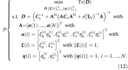
Tr(D). As done in [3], we consider Tr(D) as the relevant figure of merit and minimize it to optimize transmission and reception polarizations.
Thus, the problem of jointly optimizing transmis-sion and reception polarizations, to minimize the
MSE of estimating Xt with N diversely polarized
pulses, can be formulated as
P
RemarksActually, there exist several potential opti-mality criteria for the problem at hand, e.g.,
minim-izing the determinant of D, minimizing the
maximum eigenvalue ofDand the aforementioned Tr(D),
following: firstly, it is reasonable, as stated before and sec-ondly, we exploit the same problem formulation as in [3] and then highlight our design.
4 Optimal waveform selection
In the sequel, we will deal with the non-convex (the ob-jective is non-convex and ‖ξ(i)‖=‖η(i)‖= 1 defines a
non-convex set) optimization problemP. By
reformulat-ing the problem usreformulat-ing trigonometric parameters and the inspection of its computational complexity, we exploit the sequential minimum MSE estimation scheme to compute the optimal Tx/Rx polarizations instead of dir-ectly utilizing the minimum MSE estimation.
4.1 Problem reformulation
A first step toward the goal to tackle the optimization problem is represented by the following notations of transmission and reception polarizations. As to the transmission polarization, it can be parameterized into the following trigonometric function [2]:
ξ¼k kξ ejφQw ð13Þ complex envelope of the source signal, α denotes the rotation angle between the system coordinates and the electric ellipse axes, andβdetermines the ellipse’s eccentri-city, respectively, with the definition spaces of these trig-onometric parameters being φ∈(−π,π], α∈[−π/2,π/2],
Similarly, the trigonometric form of received polarization can be written as
η≜ejϕ ιιh
We can observe that, once ξ and η are written
into (14) and (15), respectively, Tr(D) can be
uniquely determined by trigonometric parameters {φ,α,β,ϕ,θ,ϑ}. Before proceeding further, herein we
introduce an interesting observation of Tr(D) with
respect to such parameters, as summarized in
following property.
Property 1 The initial signal phases φ and ϕ do not affect the value ofD.
ProofSee Appendix 2.
It can be seen that with Property 1, Tr(D) can be
uniquely determined by four trigonometric parameters
{α,β,θ,ϑ} instead of six trigonometric parameters {φ,α,
We can see that P1 is still a non-convex
optimization problem because the objective function
is the same non-convex function as in P.
Neverthe-less, as opposed to P, the equivalent formulation
pro-vided by P1 shows that lattice search along the
trigonometric parameters {α,β,θ,ϑ} can be employed to calculate the optimal polarization, as done in [2] and [5]. But since lattice search does not explore any optimization property, it requires a high computa-tional burden. Precisely, the computacomputa-tional complexity
is firstly exponential to the observation number N.
Also, it highly depends on the maximum point search algorithm used for {α,β,θ,ϑ}. If we use lattice search with lα,lβ,lθ and lϑ points in each dimension of the
domain space {α,β,θ,ϑ}, respectively, the relevant complexity burden is O((lαlβlθlϑ)N).
4.2 Sequential minimum MSE estimation
Since to solve P1 straightforward requires a high
computational burden, we exploit the sequential
mini-mum MSE estimation to tackle it. By insight of P1,
we can observe that it works at the case of block sig-nal polarization design, namely designing the
polariza-tions of N consecutive temporal signal samples at a
time. However, in real radar signal processing applica-tions, the returns are ongoing as time progresses. So it is reasonable to process the data sequentially in time. As to the problem at hand, the resulting solution belongs to the sequential minimum MSE estimation. Thus, by following the sequential mini-mum MSE estimation procedure in [Kay [17], Eq.
(12.47)–(12.49)], we develop the sequential minimum
MSE estimation to handle P1 as follows.
Let X^t;n denote the minimum MSE estimator based
corresponding minimum MSE matrix (just the se-quential version of (10) and (11)). Then, when the new sample y(n+ 1) is available, the estimator is up-dated as
^
Xt;nþ1¼X^t;nþKnþ1 y nð þ1Þ−aTðnþ1ÞX^t;n
; ð17Þ
where
Knþ1¼ Dna
nþ1
ð Þ
Anþ1CcAHnþ1þσ2vInþ1
nþ1;nþ1þaHðnþ1ÞDnaðnþ1Þ ;
ð18Þ
is the gain factor weighting confidence in the new data withAn+ 1= [a(1),…,a(n+ 1)]Tanda(i) having the same
definition as before and [·]n+ 1,n+ 1 denoting the n+ 1th
diagonal element of matrix [·]. In the meantime, the minimum MSE matrix is updated as
Dnþ1¼ Inþ1−Knþ1aTðnþ1Þ
Dn: ð19Þ
As to Dn+ 1, based on [Kay [17], p. 393], with n in-creasing, [Dn+ 1]ii,i= 1, 2, 3, 4, decreases and converges to a certain value. Hence, tr(Dn+ 1) is also a monotonic decreasing sequence and converges to a certain value.
4.3 Optimal waveform parameter selection
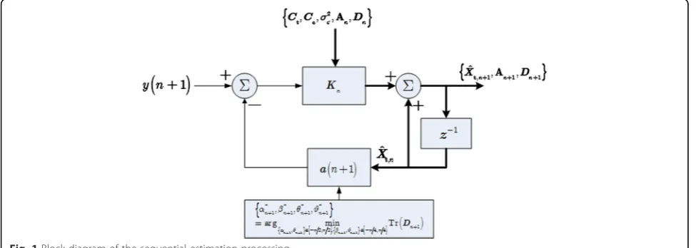
By employing the sequential minimum MSE estimation procedure described earlier, our goal is to search for the optimal Tx/Rx polarizations for every iteration, under the criterion of minimizing the Bayesian MSE-based cost function tr(Dn). As to each iteration, we still employ lattice search to compute the optimal Tx/Rx polariza-tions. Precisely, the sequential procedure to update the optimal polarizations is summarized as Algorithm 1. Also, Fig. 1 exhibits a pictorial representation of the sequential estimation processing.
Now let us examine the computational complexity of Al-gorithm 1. Let us still consider that there areNobservation samples. Different from solvingP1, Algorithm 1 is linear to
the observation numberN, with requiring the lattice search for the optimal polarizations in the domain space {α,β,θ,ϑ} in each iteration. Thus, the overall complexity is
O(lαlβlθlϑN). In comparison with the direct lattice search to
solve P1, the computation burden is greatly reduced. It is
not surprising since the proposed algorithm is sequential, namely it does not optimize for all observations and thus, it is clearly less expensive than the one proposed in (16).
5 Vector measurement system
Vector sensors, which employ two-dimensional sensors to measure both horizontal and vertical components of the electric field at each of the receivers, provide a significant improvement in performance over scalar sensors for a var-iety of applications [10, 18]. For such mentioned reason, in this section, we develop the approach to optimize trans-mission polarization of vector measurement systems by following the similar way of designing the optimal Tx/Rx polarizations for the aforementioned scalar system. In general, the derivation of such system model and the cor-responding adaptive design process follow the similar way as the model in Section 2, so it is simplified.
5.1 Vector measurement model
As to the vector measurement system with adaptive trans-mission polarization, the transtrans-mission vector ½ξh;ξvT is
allowed to be chosen freely while the reception side has both horizontal and vertical channels to separately receive horizontal and vertical polarizations of the return, respect-ively, to form a two-dimensionalvector. The scattered field is related to the incident by
yð Þ ¼t g
r2ðStþScÞξs tð−τÞ þwð Þt ; ð20Þ
complex envelope vector of noise for both polarizations, and the other parameters have the same definitions as in Eq. (1). This signal is sampled and passed through the matched filter whose output is appropriately normalized to move the effect of rg2 into the noise term. Finally, the normalized
out-put of the matched filter at the receiver is given as
y¼ðStþScÞξþv; ð21Þ
where y¼½yhyvT and v¼½vhvvT. Stacking all the
ob-servations and the noise components into column vectors, in a similar fashion to the approach used in Section 2, we obtain 2N-dimensional vectors y′ and
v′, i.e., y′¼y
, respectively. Vectors Xt
and Xc remain the same as defined earlier.
We also define the transformation matrix
T¼
So the observation vector is expressed as
y′¼TX
tþTXcþv′: ð23Þ
Thus, we obtain a similar linear model for the vector system with the scalar one. In order to make a fair com-parison, assume thatvhð Þ,i vvð Þ, andi i= 1,…,Nhave the
same power with σ22 and are uncorrelated with each
other. Then, the covariance matrix D′of Xt’s minimum MSE estimation fromy′is
D′¼ C−1
Substituting the trigonometric representation of (14) into (24) and following the same way in Section 4.1, we can prove that the initial signal phase φdoes not affect the value ofD′. Since the relevant proof can be obtained similarly as that given for Property 1, it is omitted for the sake of brevity. Hence, the optimization problem of seeking the optimal transmission polarization to
minimize the MSE of estimating Xt for vector systems
can be formulated as
P2
Similar in solvingP1, the computational complexity of
solving P2 depends exponentially on the observation
numberN, as well as the complexity burden required at
each observation, i.e., the maximum point search algo-rithm used for parameters {α,β}. Considering employing lattice search withlαandlβpoints in each dimension of
the domain space {α,β}, the required complexity is
5.2 Sequential estimation algorithm for vector systems Because of the similar reason, namely directly solvingP2
by searching for the optimal trigonometric parameters with latter search requires a high complexity burden, now in this subsection, we develop the relevant sequen-tial optimization procedure for such vector system. Let
^
Xt;n denote the minimum MSE estimator based on the
observations ½yhð Þ1 ;yvð Þ1 ;…;yhð Þn;yvð ÞnT and D′n be the corresponding covariance matrix of the estimator. Then, with the new sampley(n+ 1), the estimator is up-dated as
^
Xt;nþ1¼X^t;nþKnþ1 yðnþ1Þ−tTðnþ1ÞX^t;n
; ð26Þ
where
tðnþ1Þ ¼ ξhðnþ1Þ ξvðnþ1Þ 0 0
0 0 ξhðnþ1Þ ξvðnþ1Þ
T
;
ð27Þ
and
Knþ1¼D′ntðnþ1Þ
Tnþ1CcTHnþ1þ
σ2 v
2I2ðnþ1Þ
h i
2ðnþ1Þ;2ðnþ1Þþt
Hðnþ1ÞD′ n
tðnþ1Þ; ð28Þ
withTn+ 1= [t(1),…,t(n+ 1)]Tand [·]2(n+ 1),2(n+ 1)
denot-ing the 2(n+ 1)th diagonal element of matrix [·]. In the meantime, the covariance matrix is updated as
D′
nþ1¼ I2ðnþ1Þ−Knþ1tTðnþ1Þ
D′
n: ð29Þ
Again, as to D′nþ1, with n increasing, Dn′þ1ii de-creases and converges to a certain value. As a
conse-quence, trD′nþ1 is also a monotonic decreasing
sequence and converges to a certain value. Finally, the devised sequential optimization procedure is summa-rized in Algorithm 2.
It is worth noticing that the computational complexity
of Algorithm 2 is linear to the observation number N,
with requiring the lattice search to seek the optimal polarization in the domain space {α,β} for every obser-vation. Thus, the overall complexity is O(lαlβN).
Com-pared to handling P2 straightly with lattice search (the
corresponding computational complexity is O((lαlβ)N)),
the computation burden is greatly reduced. The reason why the proposed algorithm is less expensive than solv-ing P2 is similar as that in Algorithm 1, namely it is
se-quential and does not require optimization for all observations.
6 Numerical examples
In this section, the performance analysis of the proposed algorithms is presented. As to scalar measurement sys-tems with the joint Tx/Rx polarization optimization, we provide numerical examples to demonstrate the effective-ness of the devised algorithms, in comparison with two other polarization approaches. Additionally, we also com-pare their performances with that of the vector measure-ment system with transmission polarization optimization and highlight the advantage of the latter design.
Throughout the simulations, we generate the target and clutter covariance matrices employing a similar way as in [3]. Though the solution in [3] is criticized incor-rectly in Section 1, the approach there to generate target and clutter covariance matrices is fine. Precisely, the tar-get covariance matrix is chosen as
Ct¼aUtΛtUHt ; ð30Þ
whereUtis an arbitrary unitary matrix constructed with
the left singular vectors of a 4 × 4 matrix Mwith inde-pendent and identical distribution complex Gaussian en-tries, i.e.,M=UtΛMUr,Λt= diag(rand(1, 4)) with rand(1,
signal-to-clutter-plus-noise ratio (SCNR) with the def-inition [5]:
SCNR¼ trð ÞCt trð Þ þCc σ2v
; ð31Þ
where the clutter covariance matrix is chosen as
Cc¼UcΛcUHc; ð32Þ
withΛc= diag([0.25, 0.25, 0.25, 0.25]) andUcbeing chosen
with the similar operation to generateUt. Throughout the
simulations, we assume the noise powerσ2v= 0 dB.
Furthermore, by inspection of Eqs. (19) and (29), we can observe thatDn+ 1andD′nþ1 do not depend on the
obser-vationsyiþ1ni¼0andyiþ1ni¼0, respectively, even though in Algorithm 1 and Algorithm 2, both of them are the in-put parameters that update the estimation of target scat-tering vector X^t. Since the MSE of X^t is the figure of
merit for the optimization problem and Tr(Dn+ 1), Tr
D′
nþ1
are the objectives to be optimized for each algo-rithm, respectively, in this section, we will investigate the changes of Tr(Dn+ 1) and Tr D′nþ1
without considering
updating of X^t. As a consequence, we do not use
yiþ1
n
i¼0 and yiþ1
n
i¼0 in the simulation. Also notice that n≥4 is required for both the proposed algorithms. So we ran-domly choose f gαi 4i¼1¼ βi
4
i¼1¼f gθi 4
i¼1¼f gϑi 4i¼1¼π=8
(some other values within the definition ranges can be also used) as the initial trigonometric parameters to generateA4 andT4for Algorithm 1 and Algorithm 2, respectively.
Finally, regarding the lattice search used to seek the optimal polarizations for Algorithm 1 and Algorithm 2, set lα=lθ= 103 and lβ=lϑ= 500. By using the Monte
Carlo method, the MSEs are calculated by averaging 105
independent realizations ofCtandCc, respectively.
6.1 Scalar measurement systems
We choose the conventional polarimetric radar and the po-larimetric radar with adaptive transmission polarization as the counterparts to compare their performances with the polarimetric radar with joint Tx/Rx optimization. As to conventional polarimetric systems, the transmission side al-ternatively transmits horizontal and vertical polarizations, i.e., ξ= [1, 0]T in the current pulse and ξ= [0, 1]T in next pulse. In the reception side, the horizontal and vertical po-larizations are simultaneously received, so the reception vector satisfiesη¼pffiffiffi2=2;pffiffiffi2=2T. Therefore, the relevant MSE can be calculated by substituting the waveform pa-rameters {α= 0,β= 0,θ=‐π/4,ϑ= 0} and {α=−π/2, β= 0,θ=−π/4,ϑ= 0}, alternatively, into Algorithm 1 with the increase of observation samples and without optimal polarization search. Then, as to the scalar system with
trans-mission polarization optimization, the transmission
polarization ½ξh;ξvT is allowed to be chosen freely while
the reception polarization is fixed as pffiffiffi2=2;pffiffiffi2=2T. As such, we can employ Algorithm 1 to optimally select trans-mission polarization by fixingθ=−π/4 andϑ= 0.
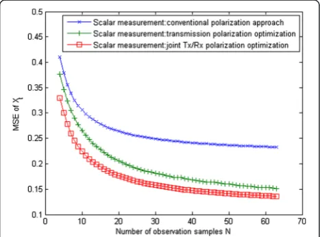
By employing Algorithm 1, Fig. 2 plots the MSEs of
the estimating target scattering matrix St versus the
number of observation samples for the aforementioned three scalar systems, with SCNR = 0 dB. As expected, the devised method monotonically reduces the MSE and converges to a certain value. On the other hand, the plots clearly show that the scalar system with joint Tx\Rx polarization optimization performs better than that with transmission polarization optimization as well as the scalar system with transmission polarization optimization showing a significant performance gain with respect to conventional polarization radars.
Additionally, Fig. 3 draws the MSE of the estimating tar-get scattering matrixStversus the SCNR, with a fixed 50 observation samples. It can be observed that, the scalar system with optimally designed Tx/Rx polarizations leads to a power gain of 4–6 dB with respect to that with only transmission polarization optimization, as well as 6–8 dB gain with respect to the conventional polarization radar.
6.2 Scalar measurement systems versus vector measurement systems
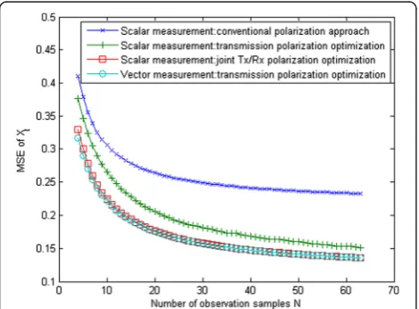
In this subsection, we compare the performance of scalar measurement systems with that of vector systems. As in Fig. 4, the MSEs of the three aforementioned scalar systems and the vector system with transmission polarization optimization versus the number of observation samples with SCNR = 0 dB are illustrated. The results highlight that the vector measurement with transmission polarization optimization has almost the same estimation performance as the scalar measurement with joint Tx/Rx polarization
Fig. 2MSE performance comparison of estimating the target scattering matrixStversus the number of observation samples,
optimization. This is because, in the former case, the receiver polarization optimization is implicitly performed. In other words, even though we perform joint optimization over both transmission and reception polarizations for the scalar sys-tem, we are still finding the best linear combination of the two received measurements at each receiver. However, com-bining them linearly need not be the overall optimal solution, even if we spend much more time on doing so. This can be avoided by retaining the vector measurements, thereby showing better performance as demonstrated in [6].
Finally, Fig. 5 shows the performance of the four systems as a function of SCNR, with the fixed length of observation sample. Again, the results demonstrate that the vector measurement system has the same performance with the scalar measurement system with joint Tx/Rx optimization.
7 Conclusions
Adaptive polarization design of polarimetric radars, for the purpose of optimally estimating the target polarization scattering vector, is studied. Starting from the problem of designing the optimal polarizations for the scalar measurement system with joint Tx/Rx polarization optimization, under considering the mini-mum MSE of the estimator as the figure of merit, a sequential method of selecting the optimal Tx/Rx po-larizations for such system is developed by owing to a suitable reformulation of the considered non-convex design problem. Furthermore, by employing a similar deviation procedure, a sequential method to select the optimal transmission polarization for the vector sys-tem with transmission polarization optimization is also devised. Since both the proposed algorithms make use of the sequential minimum MSE estimation, they monotonically decrease the MSE of the estima-tion and converge to a staestima-tionary point. The complex-ity of the proposed methods is linear with the number of outer iterations whereas at each iteration, it mainly requires the lattice search along four and two trigonometric parameters, respectively.
Several numerical examples have been provided to assess the effectiveness of the proposed methods. Pre-cisely, the performance of the scalar measurement system with joint Tx\Rx polarization optimization, the one with transmission polarization optimization and the one with conventional polarimetric design, is compared. The system with joint Tx\Rx polarization optimization shows a significant performance im-provement with respect to the one with transmission polarization optimization, as well as the conventional
polarization approach. Moreover, the numerical
Fig. 4MSE performance comparison between scalar measurement systems and vector measurement ones versus the number of observation samples, with SCNR = 0 dB
Fig. 3MSE performance comparison of estimating the target scattering matrixStversus the SCNR, with a fixed 50 observation samples
results also show that the vector measurement system with transmission polarization optimization provides the comparative estimation performance with the
scalar measurement system with joint Tx/Rx
optimization. This is because, in the latter case, the receiver polarization optimization is implicitly per-formed. But the vector measurement system requires a lower computation burden, highlighting the advan-tage of such system design.
8 Appendix 1: Proof of the failure of the proposed method in [3] to solve Tx/Rx polarizations
Before the proof, in such context, we declare that the parameter definitions and notations hereinafter have the same meaning as in [3]. In [3], the authors propose an adaptive waveform polarization method for the estimation of target scatter in the presence of clutter. The proposed algorithm, to determine the coefficients of the antenna transmission and recep-tion polarizarecep-tions, has a convex form and can be solved by employing SDP. However, the authors do not investigate whether the polarization vectors can be obtained after the convex problem is solved to
obtain A (at least such processing is absent in the
paper). In this appendix, we provide a proof that the transmission and reception polarization vectors can-not be effectively obtained through the solution of A. Essentially, the convex form is only a relaxation version of the initial problem. The proof is as follows.
Let us assume that A is already solved by employing
the proposed convex optimization in [3]. A is an m× 4
complex matrix and based on (4) and (6) of [3], its ith
Notice that the transmission polarization vectorξcan be generally parameterized as follow:
ξ ¼½ξhξvH≜ cosϕejθh sinϕejθv
; ð34Þ
wherefϕ;θh;θvg∈ −ð π;π. In a similar way, the reception
polarization vector η can be taken into the following form:
η¼ ηhηv
H
≜cosφejϑh sinφejϑv; ð35Þ
where fφ;ϑh;ϑvg∈ −ð π;π.Moreover, we also introduce
parameterized representation of the 4 × 1 complex vec-torp(ξ(i),η(i)) as follow:
Hence, by introducing (34), (35), and (36) into (33), we obtain the following equations:
ξð Þi
Furthermore, (37) can be recast into two equation systems, namely
As to (38), after some algebraic manipulations and in-verse trigonometrical transform, we can transform (38) into the following equations:
ϕ−φ¼ arccosðpi1þpi2Þ
We can see that (40) is an over-determined equa-tion system. By employing the least-square method,
we can search for the “approximately” solution of ϕ
and φ as
ϕ¼0:25ðarccosðpi1þpi2Þ þarccosðpi1−pi2Þ þ arcsinðpi4−pi3Þ þarcsinðpi3þpi4ÞÞ
φ¼0:25ðarccosðpi1−pi2Þ−arccosðpi1þpi2Þ þarcsinðpi3þpi4Þ−arcsinðpi4−pi3ÞÞ :
As to (39), after some algebraic manipulations, we ob-tain the following equation system:
θh−θv¼βi4−βi1 arbitrary value within (−π,π], the first equation may conflict with the second equation when βi4−βi1≠βi2
−βi3and the third one may contradict the fourth one
when βi1−βi3≠βi4−βi2.
As a consequence, the transmission and reception polarization vectors cannot be always effectively solved
based onA. The proof is concluded.
RemarksLemma 2.1 of [10] provides a three-parameter representation of the signal polarization, which has a
dif-ferent form from our so-calledtwo-parameter “general”
formulation (34). In the appendix, we do not implement such three-parameter representation since the proof will become more cumbersome and prolix by employing the new one. But the study shows (not shown here) that the question of conflict arises again with the use of the three-parameter representation.
9 Appendix 2: Proof of Property 1
Let us first introduce the following new variables for (11)
B ¼ σ−1
Then (11) can be written into
D−1
1 ¼C−t;11þBH BBHþIN
−1
B: ð44Þ
Using the matrix inversion lemma, we obtain
I4þBHB
Meanwhile, substituting (14) and (15) into the second term of (8), the following equation is obtained
A¼UM; ð47Þ
Therefore, the initial signal phases φ and ϕ do not
affect the value ofD. This concludes the proof.
Competing interests
The authors declare that they have no competing interests.
Acknowledgements
The authors would like to thank Mr. John Lucynski for providing some comments on how to correct the language. This work was also supported by the National Natural Science Foundation of China (Nos. 61401488, 61501475, and 61490692).
Received: 28 March 2015 Accepted: 12 November 2015
References
1. D Giuli, Polarization diversity in radars. Proc. IEEE74(2), 245–269 (1986) 2. J Wang, A Nehorai, Adaptive polarimetry design for a target in
compound-Gaussian clutter. Signal Process.89, 1061–1069 (2009) 3. J-J Xiao, A Nehorai, Joint transmitter and receiver polarization
optimization for scattering estimation in clutter. IEEE Trans. Signal Process.57(10), 4142–4147 (2009)
4. DA Garren, AC Odom, SU Pillai, JR Guerci, Full-polarization
matched-illumination for target detection and identification. IEEE Trans. Aerosp. Electr. Syst.38(3), 824–837 (2002)
5. M Hurtado, A Nehorai, Polarimetric detection of targets in heavy inhomogeneous clutter. IEEE Trans. Signal Process.56(4), 1349–1361 (2008) 6. S Gogineni, A Nehorai, Polarimetric MIMO radar with distributed antennas
for target detection. IEEE Trans. Signal Process.58(3), 1689–1697 (2010) 7. J Liu, Z Zhang, Y Yang, Performance enhancement of subspace detection
with a diversely polarized antenna. IEEE Signal Process. Lett.19(1), 4–7 (2012) 8. J Liu, Z Zhang, Y Yang, Optimal waveform design for generalized likelihood
ratio and adaptive matched filter detectors using a diversely polarized antenna. Signal Process.92(4), 1126–1131 (2012)
9. M Hurtado, T Zhao, A Nehorai, Adaptive polarized waveform design for target tracking based on sequential Bayesian inference. IEEE Trans. Signal Process.56(3), 1120–1133 (2008)
12. CVX Research, Inc. CVX: Matlab software for disciplined convex programming, version 2.0. http://cvxr.com/cvx, April 2011
13. M A Richards, J A Scheer, W A Holm,Principles of Modern Radar: Basic principles(IET Digital Library, 2010)
14. A Aubry, A De Maio, A Farina, M Wicks, Knowledge-aided (potentially cognitive) transmit signal and receive filter design in signal-dependent clutter. IEEE Trans. Aerosp. Electron. Syst.49(1), 93–117 (2013) 15. F Gini, A De Maio, L Patton,Waveform design and diversity for advanced
radar systems(Institution of Engineering and Technology, London, 2012) 16. A Aubry, A De Maio, M Piezzo, A Farina, M Wicks, Cognitive design of the
receive filter and transmitted phase code in reverberating environment. IET Radar Sonar Navig.6(9), 822–833 (2012)
17. SM Kay,Fundamentals of statistical signal processing: estimation theory
(Prentice-Hall, New Jersey, 1993)
18. A Nehorai, E Paldi, Acoustic vector-sensor array processing. IEEE Trans. Signal Process.42(9), 2481–2491 (1994)
19. GE Box, WG Hunter, JS Hunter,Statistics for experimenters(John Wiley & Sons, New York, 1978)
Submit your manuscript to a
journal and benefi t from:
7Convenient online submission
7Rigorous peer review
7Immediate publication on acceptance
7Open access: articles freely available online
7High visibility within the fi eld
7Retaining the copyright to your article