Lists in a Lighthouse

University of South Carolina

Scholar Commons

Theses and Dissertations

2015

Tree-Sway Frequency And The Turbulent

Co-Spectral Gap In A Dense Canopy Environment

Katherine L. Ertell

University of South Carolina

Follow this and additional works at:https://scholarcommons.sc.edu/etd

Part of theGeography Commons

This Open Access Thesis is brought to you by Scholar Commons. It has been accepted for inclusion in Theses and Dissertations by an authorized administrator of Scholar Commons. For more information, please [email protected].

Recommended Citation

TREE

-

-

By

Katherine L Ertell

Bachelor of Science Valparaiso University, 2012

Submitted in Partial Fulfillment of the Requirements

For the Degree of Master of Science in

Geography

College of Arts and Sciences

University of South Carolina

2015

Accepted by:

April Hiscox, Director of Thesis

Greg Carbone, Reader

Sarah Battersby, Reader

A

Thank you to my wonderful family—Mom, Dad and Andy—for your endless support for

my crazy dreams and passions that have now turned into a career that I love and look

forward to each and every day. I could not have done it without your direction. You all

truly are the best role models I could have ever asked for.

Thank you to my wonderful Graduate Advisor, Dr. April Hiscox, for your constant

encouragement and patience as I juggled moving far from home and getting my first job

all in the last two years. I could not have accomplished this without your guidance.

Thank you to my readers, Greg Carbone and Sarah Battersby, for sharing your expertise

and helpful feedback in this project.

Thank you to my undergraduate professors at Valparaiso University, Dr. Teresa

Bals-Elsholz and Dr. Bharath Ganesh-Babu, who pushed me to pursue my Masters degree at

the University of South Carolina and helped me to find my niche in the field of

A

Today, knowledge of canopy turbulence comes solely from field observations.

However, measurements or field observations that are taken at a specific location within

the canopy cannot accurately capture the interaction of the wind and the canopy it

crosses. Without this complete picture of the atmosphere, the temporal fluctuations that

exist in turbulent flows cannot be understood. From an atmospheric perspective, the

complex structure of forests significantly influences turbulence in the atmospheric

boundary layers (ABL) by consistently imposing both mechanical and thermal forces.

This study explores the temporal and spatial characteristics of tree-sway motions and

their aerodynamic interactions with coherent turbulence wind fields in a forest (Howland

Forest, ME). Flux calculations from tower data, such as in this experiment, require the

researcher to choose a timescale to define fluctuations, however since the atmosphere

typically contains motions and coherent vertical transports on a multitude of timescales;

the selection of it is not always straightforward. This study will aid in answering whether

or not there is a correlation between average stem sway frequency and the turbulent

co-spectral gap in a forest environment. Results were achieved by using a multi-resolution

decomposition (MRD) technique to find a day-time specific time scale and then

examining the tree's frequencies at that time scale through a Fourier transform to

determine if MRD can find an appropriate time scale of coherent motions. Through a

mapping comparison, the sub-mesoscale motions of a canopy atmosphere and their effect

coherence was seen when examining motion on time scales greater than the co-spectral

gap, which would include meso and sub meso scale motions. Frequency proved to be a

good variable for mapping the wind. Overall this work highlights the usefulness of

dynamic maps for displaying data and better understanding rapidly changing spatial

patterns that may have been missed otherwise. This will eventually lead to incorporating

canopy motion physics into bigger climate models, as well as providing an explanation to

T

C

ACKNOWLEDGEMENTS ... iii

ABSTRACT ... iv

LIST OF FIGURES ... vii

LIST OF SYMBOLS ... viii

LIST OF ABBREVIATIONS ... ix

CHAPTER 1:INTRODUCTION……….1

OBJECTIVES ...11

CHAPTER 2:METHODS ...14

DATA...14

DATA ANALYSIS ...17

DATA PRE-PROCESSING ...18

DATA SELECTION ...18

IDENTIFICATION OF TIME SCALE ...20

IDENTIFYING TREE MOTION ...26

DYNAMIC MAPPING ...27

CHAPTER 3:RESULTS ...29

CHAPTER 4:CONCLUSIONS AND DISCUSSIONS ...37

REFERENCES ...39

L

F

FIGURE 2.1:TREE MODEL ...15

FIGURE 2.2:WIND ROSE ...16

FIGURE 2.3:MRD2011-05-27 ...24

FIGURE 2.4:MRD2011-05-30 ...25

FIGURE 3.1:FFT2011-05-27 AT GAP SCALE ...29

FIGURE 3.2:FTT2011-05-27 AT DOUBLE GAP SCALE ...31

FIGURE 3.3:FREQUENCY CHANGE MAP 12011-05-27 AT GAP SCALE ...32

FIGURE 3.4:WIND DIRECTION AND SPEED PLOT 2011-05-27 ...33

FIGURE 3.5:FREQUENCY CHANGE MAP 12011-05-27 AT DOUBLE GAP SCALE ...33

FIGURE 3.6:FREQUENCY CHANGE MAP 22011-05-27 AT GAP SCALE ...34

FIGURE 3.7:FREQUENCY CHANGE MAP 22011-05-27 AT DOUBLE GAP SCALE ...35

L

S

VERTICAL LENGTH SCALE

h CANOPY HEIGHT

TS SONIC TEMPERATURE

u, v, w WIND COMPONENT

u’w’ VERTICAL KINEMATIC TURBULENT FLUX DENSITY OF THE X-DIRECTION

(STREAMWISE) MEAN MOMENTUM (ΡU)

( )

s h h

L

A

CHAPTER

1:

I

Wind flow within forest canopies is important for studies of atmospheric waves

(Lee and Barr, 1997) and turbulence exchange (Finnigan, 2000). In the boundary layer,

transport of quantities such as moisture, heat, momentum, and pollutants is dominated in

the horizontal direction by the mean wind and in the vertical direction by turbulence.

Turbulent winds drive scalar dispersion and exchanges of heat and mass between plants

and their surrounding atmospheric environment (Moneith, 1981). These exchange

processes and their influences on the physiological functions of terrestrial plants continue

to be significant components of global hydrological and carbon cycles (Monsi et al.,

1973, Baldocchi et al., 2002, Law et al., 2002).

More than a third of the Earth’s surface is covered by vegetation. Vegetation

repeatedly influences the climate through the exchanges of energy, water, carbon dioxide,

and other chemicals found in the atmosphere. These particular exchanges and their

associated wind transport aid in furthering the accuracy of climate models today.

However, understanding and quantitatively analyzing the wind flow in the lowest section

of the boundary layer becomes even more complex due to the inherent thermal and

mechanical influence of the canopy elements (Raupach et al., 1996). Understanding the

processes driving vegetation–atmosphere exchange would aid in a clearer understanding

problems which arise in agricultural and natural resource management, including

catastrophic wind damages to crops and forests (Foster and Boose, 1992).

Forest ecosystems are structurally more complex, and live much longer than

agricultural crops. They therefore continuously adapt to local wind conditions over many

years. The susceptibility of a forest canopy to wind forces is strongly linked to not only

its structure (Canham and Loucks 1984) but also its thigmic response to wind induced

bending stresses (Telewski and Pruyn 1998, Henry and Thomas 2002). Investigations

into the relationship between forest canopy structures and their thigmic responses to local

wind regimes are only in their infancy (Rudnicki et al. 2004). Catastrophic windstorms at

a landscape scale (Boose et al. 1994) are predicted to increase the frequency and size of

forest disturbances in the near future (Peterson 2000). Even with that pressing

knowledge, uncertainties remain regarding the interactions between changing forest

disturbance dynamics and predicted climate change patterns. (Dale et al. 2001). A

mechanistic understanding of the dynamics of individual tree stability and failure (Baker

1995, James et al. 2006) is critical to predict how forest structures and functions (e.g.,

succession) would respond to future global environmental changes, in particular more

frequent and stronger windstorms—before they occur (Emanuel 2005, Trapp et al. 2007).

From an atmospheric perspective, the dynamic and complex construction of

forested ecosystems has significant influences on turbulence structures in the atmospheric

boundary layers (ABL). A forest canopy consistently imposes energy in both mechanical

and thermal forces. The lower layer of the atmosphere responds directly to changes in

an hour or less. Examples of these forces or changes that can influence the ABL are:

frictional drag, evaporation and transpiration, heat transfer, pollutant emission, and

terrain induced flow modification.

In Roland Stoll’s An Introduction to Boundary Layer Meteorology (1988), he

explains that wind in the boundary layer can be divided into three categories: mean wind,

turbulence, and waves. Each can exist separately, or in presence of any others within the

boundary layer of the atmosphere. Mean wind, often connected to advection, is

characterized as very rapid horizontal transport. Rapid horizontal winds on the order of 2

to 10m/s are often found in the ABL. Turbulent fluxes can be defined loosely as the

collection of links between random fluctuations in velocity and scalars that effectively

transport energy from the Earth’s surface into the troposphere. Waves are winds that

transport little heat, humidity, and other scalars, but effectively transport momentum and

energy. Waves can serve as an initiator of turbulence as they often cause enhanced wind

shears in localized regions. In the boundary layer, unlike the rest of the atmosphere, there

is an abundance of turbulence near the surface. In the canopy roughness sublayer (CRSL)

(Kaimal and Finnigan 1994), a layer that extends upward from z=h (vertical=canopy

height) to about 2h (twice the canopy height), turbulence characteristics, momentum

transfer, and the transport, diffusion and deposition of scalars and particles are strongly

influenced by canopy morphology.

In the lowest 10% of the ABL, called the “atmospheric surface layer” (ASL ), a

series of assumptions are made to describe turbulent wind behavior. We may assume that

fluctuating turbulent velocities U,v,w in the x,y,z directions, respectively. The term U’w’,

the vertical kinematic turbulent flux density of the x-direction (streamwise) can be used

to show turbulence in the ASL. When the ASL is turbulent, then U′w′ will be constant

with height. The assumption of a constant vertical flux allows the use of these constant

fluxes as parameters in a set of relationships known as Monin–Obukhov Similarity

Theory (MOST). Work over the last several years by Patton and Finnigan (2009), and

Vickers and Mahrt (2002), has shown that MOST is not always applicable, particularly at

night in canopies.

Under these conditions, the downward turbulent momentum flux u′w′ continually

decreases. This is can be attributed to that mean streamwise momentum (ρu), which is the

momentum absorbed through the aerodynamic drag on the plants. Therefore, within the

canopy, the similarity scaling leading to the log-law and MOST is no longer applicable.

This means that there is not a direct connection between scalar turbulent fluxes and scalar

local gradients. A basic understanding of the nature of canopy turbulence can make this

difference more clear.

Turbulence, the gustiness superimposed on the mean wind, can be visualized as

consisting of irregular swirls or motion called eddies. Turbulence can also be thought of

as a collection of many different sized eddies all superimposed on each other. The

turbulence spectrum is therefore made up of the relative strength of these different scale

eddies. Almost all of the boundary layer turbulence is caused or generated by forcings from the earth’s surface. An example of this is solar heating. On sunny days, the ground

classified as large scale eddies. Obstacles such as trees and buildings affect the flow by

deflecting it, causing turbulent wakes adjacent to, but downwind from an obstacle.

Information on the size of eddies and on the scale of motions in the boundary

layer is needed to understand turbulence. Unfortunately, capturing a snap shot picture of

the ABL is not an easy task. Canopy sized turbulent eddies have been reported in

previous studies (Raupach, Finnigan et al. 1996), however, the turbulent eddies-- which

are influenced by the motion of the canopy elements-- remain poorly explored due to lack

of detailed understanding of tree motions. Improved understanding of turbulence

structures and modeling of turbulent transport and diffusion in the CRSL are needed to

understand the flux exchanges within and above a canopy (Gardiner, 1995).

When questions of plant canopy turbulence first appeared, researchers assumed it

could be treated like boundary layer turbulence with a few additions of fine scale eddies

that were generated by obstacles. By the 1970s, it had become clear that the dominant

eddies in plant canopy turbulent flows are much larger than the added plant element size

researchers had considered. After discovering that the addition would not account for the

difference, it took more than two decades of research to account for the generated canopy

drag that is caused by the plant elements rather than as friction on the ground (Finnigan,

2000).

However, it wasn’t just as simple as incorporating canopy drag. The distribution of

mean velocity in the canopy air is not only due to canopy drag, but instead is the result of

Canopy drag varies with height and depends on both the foliage distribution as well as

the velocity field itself in a particular forest or terrain. Similarly, the within-canopy

distribution of scalar concentrations results from a balance between turbulent transfer and

the distribution of scalar sources and sinks. As Patton and Finnigan note (2012), the

location of these scalar sources/ sinks are determined by three factors: (1) solar radiation

as it filters through the foliage, (2) the biological state of the plants such as their access to

soil water, and (3) the ambient concentrations of temperature, humidity, CO2, and other

scalars in the canopy airspace. Recent research (Rudnicki, 2004) also suggests that the

motion of canopy elements may also play a role, although this is difficult to measure.

To fully understand spatial wind fields, it would be necessary to take

measurements at many locations. This is often not possible and it is easier to make

measurements at one point in space over a long period of time. In 1938, G. I. Taylor suggested that, “for some special cases, turbulence can be considered to be frozen as it

advects past a sensor. Thus, the wind speed could be used to translate turbulence

measurements as a function of time to their corresponding measurements in space.” However, Powel and Elderkin pointed out in 1974 that “turbulence is not really “frozen”

and Taylor’s simplification is thus useful only for those cases where the turbulent eddies

evolve with a timescale longer than the time it take the eddy to be advected past a sensor.”

Raupach and Thom (1981) state that second-order closure models provide the best

hope to replace local-diffusion theory which is seriously deficient in the canopy, and that

the majority of ensemble average models at various orders of closure for airflow in the

CRSL (Wilson and Shaw 1977, Katul et al. 2004) do not consider plant motions. It is

currently unclear how much of the reported discrepancies between measured and

modeled velocity variances near the canopy top (Wilson and Shaw 1977) could be due to

ignoring plant waving in these models.

Experimental findings later underscore the importance of modeling wind-driven

plant motion. Finnigan and Mulhearn (1978) argued:

“Although the motions of individual wheat and barley stalks are excited by a turbulent wind, single stalks vibrate at a particular and well defined natural frequency, which enables them to be treated as resonant cantilevers, whose elastic properties can be measured by well-established engineering techniques”.

The simple model that Finnigan and Mulhearn (1978) developed was able to simulate

the influence of vegetation density observed in a wind tunnel experiment indicating that

the effect of the waving stalks is seen as a strong peak at the waving frequency in the

power spectrum of streamwise velocity fluctuations. This peak is completely absent in

the case of a sparse model canopy (Finnigan and Mulhearn, 1978).

Other studies have explored the use of laboratory simulations where much of the

turbulence work has been performed in laboratory tanks, usually using a liquid such as

water to simulate an environment—or a forest terrain in this case. Although there has

been some success in laboratory studies, there have only been a select few that simulate

larger phenomena. Wind tunnels have also been used to observe the flow of neutral

adequately simulate the typical daytime and nighttime boundary layer characteristics.

(Finnigan et al, 2009)

One unique approach of handling extreme wind events involves simulations of the

dynamic response of trees to the wind. (Lee, 2000). It is recognized that wind damage to

trees is most likely to occur at high wind speeds and when the excitation frequency

(frequency of wind gusts) coincides with the natural frequency of sway vibrations. The

resonance is considered to occur if the spectral peak frequency of the velocity time series

matches the natural frequency of sway vibrations (Mayer, 1989; Gardiner, 1994; Wood,

1995; Peltola, 1996).

One of the most striking examples of wind-induced plant motions, which is of most

interest in this study, is the honami (in Japanese, “ho” = “cereal”, “nami” = “wave”),

which refers to ocean-wave-like motions of cereal crops on windy days observed over a

half century ago. Several field observations (Finnigan and Mulhearn 1978) provided

some of the earliest qualitative and quantitative evidences on the significant aerodynamic

interactions between waving plants and CRSL turbulence. Analyses of movie films of

waving stalks in a barley (Finnigan and Mulhearn 1978) and a wheat field (Finnigan

1979) drew the following picture: when a honami event took place, the crop field was

divided into patches of coherent waves with abrupt and arbitrary phase differences

between adjacent patches. Individual patches were 15-20h (h is mean stalk height) in

downwind extent, 5-6h in the crosswind extent, and retained their identity for about 5

seconds on average. Five distinct crests were seen in any patch so that the wavelength is

a crest at a point in space) is 4 (Finnigan and Mulhearn 1978) to 1.8 (Finnigan 1979)

times the mean velocity at the canopy top. These spatial and temporal characteristics

suggest that honami events are one of the first records of canopy motion that are driven

by large coherent wind gusts.

Another, more recent, example is an experiment in a dense spruce forest

(Gardiner 1994), which also showed that momentum transport and tree motions are

dominated by intermittent sweep/ejection events associated with honami waves moving across the forests. Gardiner’s (1994) spectral analysis indicated that trees efficiently

absorb energy at the resonant frequency and short-circuit the inertial energy cascade.

A noteworthy theoretical development reviewed in Finnigan (2000) is the proposal by

Raupach et al. (1996) that the CRSL is more analogous to a plane-mixing-layer (PML)

than a boundary layer as originally believed. This is mainly based on common features

observed in both types of flows: an inflection point in the mean velocity profile, similar

ratios between components of the Reynolds stress tensor, the relative role of sweeps and

ejections, length scales of active turbulence, and that dominant large eddies are the results

of an instability in the ABL due to the inflected mean velocity profile. A vertical length

scale: , where and are the mean velocity and its vertical

gradient at the canopy top, is used to distinguish the inactive ( ), active ( ) and

fine-scale ( ) turbulence. The effect of vegetation density is such that is around

0.1h, 0.5h and h for dense, moderate and sparse canopies. A main effect of the large

inactive eddies is to make the active canopy-scale eddies intermittent. Each large-scale

(

)

s h h

L =U ¶ ¶U z Uh

(

)

s

L

>>

s

L

gust initiates a “wave packet” of several canopy-scale coherent eddies with a streamwise

separation of ( ), which varies from instance to instance of

large-scale gusts.

However, the PML analogy is incomplete for a CRSL that is embedded in the ABL.

There is distinct asymmetry above and below the inflection point near the canopy top.

Different interpretations (Finnigan and Shaw 2000, Watanabe 2004) of the relation

(interactions, mechanisms) between the large-scale gusts from the outer part of the ABL (Finnigan 1979) and the “wave packet” or train of several canopy-scale eddies (Raupach

et al. 1996) remain to be reconciled and fully understood. Interactions between buoyancy forces and “inflectional instability” need to be further investigated. Both earlier (Finnigan

and Mulhearn 1978, Finnigan 1979) and more recent (Py et al. 2005) experiments in and

above short crops observed that the wavelength of honami waves increases with

increasing mean wind speed.

Previous linear models are only a small step towards a full understanding of the

canopy wave dynamics because, in reality, shear-generated waves can quickly grow out

of the linear phase. One feature evident of almost all canopy wave events is the existence

of a monochromatic wave frequency.

A key factor of the equation is still missing. Although oscillations of free-swaying

plants and trees have been explored (Mayer 1987, Milne 1991, Gardiner 1992, Speck and

Spatz 2004), tree sway within a dense forest remains poorly understood. This is primarily

due to complex sway damping factors (Milne 1991, Rudnicki et al. 2008) and the

x mLs

difficulty of quantifying group sway (Mayer 1987, Gardiner 1992). More recently,

Rudnicki et al. (2008) reported that the sway frequency for a group of slender trees

(experiencing many intense crown collisions) decreases with increasing wind speed but

did not change for a group of stout trees (experiencing few and light collisions), and that

collisions between adjacent trees enhance damping and reduce sway energy. Previous

work at this field site has shown that distribution of sway frequency over the canopy

closely matched the associated spatial distribution of slenderness. (Rudnicki, Personal

Communication)

Modeling a forest canopy flow under very stable conditions (intermittent turbulence

regime) is a challenging task. (Lee, 2000). The prominent problem arises from the

difficulty in finding an interval suitable for performing the Reynolds averaging when the

turbulence is globally intermittent (Mahrt, 1999). Because static stability plays an

important part in the flow dynamics, a successful model must include a proper

parameterization of the heat exchange between the air and the plants. Mahrt et al. (2001)

discovered a spectral gap, which delineated turbulence and mesoscale motions by

examining what is known as the multi-resolution (MR) spectra (variances) of the wind

components for a variety of different tower datasets. This spectral gap is the key to

understanding the dynamic atmosphere of a forest environment.

OBJECTIVES

A large hole exists between forest meteorology studies-- which traditionally are

concerned with microscale processes (about 1 km)-- and everyday mesoscale

several tens of kilometers. In principle, mesoscale flow models are the desirable tool for

studies of wind and turbulence in complex terrain, but the cost of running such models

for wind damage assessment is prohibiting. With such a large variety of scales involved

in a complex terrain of a forest and the tremendous variability in the vertical element of a

canopy a large array of sensors including airborne platforms and remote sensors would be

required to understand all the motions in a forest canopy. The relatively large costs have

limited the scope of many field experiments and only a few general-purpose, large scales

boundary layer experiments have been conducted. (Finnigan et al, 2009) Therefore, it

remains an open question whether the mesoscale models can generate accurate wind

fields near the tree canopy (Lee, 2000).

This work examines the temporal and spatial characteristics of tree-sway motions and

their aerodynamic interactions with coherent turbulence wind fields in a forest. These

steps are aimed to answer my hypothesis that there is a correlation between average (or

local) sway frequency and the turbulent co-spectral gap in a forest environment.

1) Test the hypothesis by using a multi-resolution decomposition technique to

find a night-time specific time scale and then.

2) Examine the tree’s fundamental peak frequencies at that time scale through a

Fourier transform.

3) Determine if this is a successful way of finding representing the scale of

coherent motions which occur in the boundary layer of the atmosphere.

4) Dynamic map frequency changes of trees to identify coherent atmospheric

The focus of this particular project will be to further investigate the aerodynamic

interactions between tree sway motions and CRSL wave turbulence in and above a

CHAPTER

2:

M

DATA:

All wind and tree-sway data used in this research project were collected at the

Howland Forest in Maine, USA, approximately 35 miles north of Bangor (45.238◦ N– 68.664◦ W, elevation of 48 m). It is the site of an AMERIFLUX tower as well as a

number of other instruments (Hollinger et al., 1999). The topography of the site is very

flat with a long and uniform fetch. The region is categorized as Acadian plain and lies in

the Penobscot River flood plain. The site is a relatively, evenly aged stand of old growth

trees, approximately 130 years old, with a species mix dominated by red spruce and

eastern hemlock. The study area is a circle with a diameter of 150m. All trees within the

study area with a diameter at breast height (DBH) greater than 10 cm were tagged; and

their species, tag number, and DBH were recorded. A total of 1615 trees were included in the survey. The trees’ horizontal and vertical positions were measured relative to a site

datum using a Leica (TCR 307) total station and recorded with a Trimble data logger

running Survey Pro software (Tripod Data Systems). Tree height was measured using an

Impulse Laser Rangefinder (Laser Technology Inc., Centennial, CO) and the average

canopy height in the measurement area is 20.6 meters. Using a nominal grid spacing of

10 meters, the dominant or co-dominant tree in each grid was instrumented with a

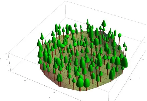
clinometer to measure tree stem displacement. Figure 2.1 shows a computer-generated

Figure 2.1: A computer generated model of the instrumented trees based on tree height, species and crown measurements.(Courtesy of M. Rudnicki, The University of

Connecticut)

This work is part of a larger study designed to understand the interactions

between tree sway and turbulence in the canopy (Granucci et al., 2013). The tower

arrangement was chosen based on the predominant wind flow from west to east seen at

Figure 2.2: Wind direction distribution for 30-minute averages of winds measured above canopy during daytime convective conditions.

Each tower at the site was equipped with three CSAT3 sonic anemometers

(Campbell Scientific, Inc., Logan, Utah). Each component of the wind speed (u, v, w)

and sonic temperature (TS) was sampled at 10Hz. For this work, data from the central

tower was utilized. The anemometers were mounted at heights of 21.4m, 15.1m, and

8.0m on a 27.5m tall, triangle frame tower (Model 25G, Rohn, Peoria, IL). The top

anemometer was mounted just above the canopy, within the CRSL. The middle

anemometer was placed near the center of the live crown and the bottom was mounted

just below the live crown. All anemometers were mounted pointing north. Instruments

were operated nearly continuously from August of 2009 to December 2011.

Tree sway on the site was measured using biaxial clinometers (Model 900,

Applied Geomechanics) mounted just below the live crown height, an approximate height

ideal for tree sway measurement because their response time is much faster than tree

sway velocities and they were easily attached to the tree’s stem. A total of 149 trees were

equipped with clinometers. Clinometer data was stored as raw voltage values and

converted to displacement values in meters using calibrations for each individual sensor.

DATA ANALYSIS

To test the hypothesis, the collected data went through several analysis steps. The

first of these steps was to use the turbulent wind measurements to identify a potential gust

frequency time step. The appropriate time step, which was determined by the MRD

method (Vickers and Marht, 1997), depends on the average wind speed of each particular

night, and therefore cannot be satisfied with a generic timescale for the entirety of the

experiment, like many researchers have assumed before (Raupach, 1989; Shaw, 1992).

Once the corresponding time step was determined, that period was used to find the

change in the fundamental peak frequency of each individual tree over the course of the

night. The fundamental peak frequency of each tree was found by using the Fast Fourier

Transform Method. Performing a Fast Fourier Transform on each individual tree gives a

picture of the universal motion of the trees, at the predetermined time scale, throughout

the forest. The changes in the determined peak frequencies were then dynamically

mapped to help identify coherent structures—proposed at the predetermined time scale.

For comparison, the FFT was also be performed on a timescale double of that found by

the MRD, the resulting dynamic maps were compared to the original maps. For this

work a visual comparison was used to identify coherency. A more quantitative analysis

the gap-scale time step will show that the data revealed more coherencies in tree motion

than those at the longer timescale.

A. DATA PRE-PROCESSING

Prior to analysis for this experiment, the angular tree sway data were normalized

and converted to displacement in order to assess the quality of the data in meters. Data

sets were normalized to a zero resting position by identifying an eight hour time period

with very low winds speeds (average 0.23m/s), with this average angle subtracted from

the data sets used in the analysis. Displacement in meters was then calculated from the

normalized tilt angle using the equations specified in Rudnicki et al (2001). The x and y

displacements were then resolved into a single horizontal displacement of the center of

gravity of the live crown. Center of gravity for each tree was assumed to be half the live

crown height (Long and Smith, 1992), which was calculated by subtracting the sensor

mount height from the total tree height.

B. DATA SELECTION

Since the work presented here is exploratory, only a small subset of the data was

used. The selection was made primarily on the time of day as well as the season (keeping

in mind snow covered trees). During the daytime the atmosphere is very unstable which

makes the majority of wind events smaller and not as widespread. Unstable air gives way

to rising motion and rising motion will affect heat fluxes, causing wind events to be more

spread out vertically rather than horizontally during the night. Also, in the evening the

that linger over night elongated and therefore condensing all of the associated energy into

a smaller and long time scale. For this reason, the events should be more recognizable at

night. Also, as a result of the nocturnal jet, the turbulence found at nighttime in the static

boundary layer sometimes occurs in relatively short bursts and can cause mixing

throughout the entire layer.

Vickers and Mahrt (2001) speculated that:

“When relating these fluxes to the local mean wind shear and temperature stratification, as in similarity theory, the prescribed timescale would ideally include transports on all turbulence timescales and exclude all mesoscale and larger motions. Mesoscale motions do not obey similarity theory and are poorly sampled on time scales of a few hours or less. Including mesoscale transport in calculated fluxes potentially degrades similarity relationships (Smedman 1988). This degradation is expected to be most significant for stable conditions, where the turbulent fluxes are small and inclusion of the mesoscale contribution can dramatically change the magnitude and even the sign of the calculated flux. In unstable conditions the turbulent flux is much larger, and therefore inadvertent inclusion of mesoscale transport is thought to have less impact on the calculated flux.”

This lead this project to look more closely at nighttime data, rather than daytime, so that there is a better change of “catching” some of the elongated eddies events that

enter the study area and pass by the towers.

Typically, these eddies are categorized best in high wind speed events, but for

purposes of this study we want to make sure to reduce the miscellaneous changes in

fundamental frequencies that may have been brought on by collisions in the upper

canopy. Without a collision factor we would ideally use high wind speed days, but will

use moderate wind speed days in hopes of catching coherency, but eliminating the

Given these criteria two nights were selected for analysis. Both were chosen for

the moderate average wind speeds following previous studies, which suggested eddies

were more visible when winds were higher and/or more turbulent. Thirty minutes

averages of horizontal wind speed, U, were examined for the entire study period. Two

nights were chosen based on sustained winds greater than 1.5m/s. These two nights were

May 27, 2011, which had an average wind speed of 3m/s and May 30, 2011, which had

an average wind speed of 2.4m/s.

C. IDENTIFICATION OF TIME SCALE

Flux calculations from tower data require the researcher to choose a

timescale to define the fluctuations. The calculated flux includes all scales of motion

from the smallest resolved by the instrumentation up to the specified averaging timescale,

and therefore, the calculated flux depends on the choice of the research. Differences in a

selection of a timescale may contribute to some of the differences between studies,

especially for the stable boundary layer. For example, while studying similarity

relationships, one might attempt to remove all non-turbulent contributions to the fluxes,

while for balancing surface energy budgets one might want to include heat fluxes at

larger timescales, regardless of their origins. Since the atmosphere typically contains

motions and coherent vertical transports (fluxes) on a wide range of timescales, the

cospectral gap varies in the literature, where a typical value is ~30-40 seconds. (Vickers

and Mahrt, 1997)

The scale dependence of the flux often reveals a cospectral gap region that

separates the turbulent scales of the cospectra from the mesoscale transport (Smedman

and Hogstrom 1975; Stull 1990). These mesoscale flows can include deep convection,

large roll vortices and local circulations due to topographical or surface heterogeneity. In

stable flows, mesoscale motions can include internal gravity waves, drainage flows, and

other less known motions. Wave-turbulence interactions at timescales as small as a few

hundred seconds have been observed to cause both gradient and counter gradient heat

fluxes in very stable conditions (Smedman 1988; Sun et al. 2002).

When relating fluxes to the local mean wind shear and temperature stratification,

as in similarity theory, the prescribed timescale would ideally include transports on all

turbulence timescales and exclude all mesoscale and larger motions. Mesoscale motions

do not obey similarity theory and are poorly sampled on time scales of a few hours or less

(Mahrt et al. 2001). Including mesoscale transport in calculated fluxes potentially

degrades similarity relationships (Smedman 1988). This degradation is expected to be

most significant for stable conditions, where the turbulent fluxes are small and inclusion

of the mesoscale contribution can dramatically change the magnitude and even the sign

of the calculated flux. In unstable conditions the turbulent flux is much larger, and

therefore inadvertent inclusion of mesoscale transport is thought to have less impact on

One method of choosing a timescale is Multi-resolution decomposition (MRD)

(Vickers and Mahrt, 2006). A multi-resolution decomposition was applied to the raw

anemometer data for each night to find the cospectral gap scale-- the timescale that

separates turbulent and mesoscale fluxes of heat, moisture, and momentum between the

atmosphere and the surface. It is desirable to partition the flux because turbulent fluxes

are related to the local wind shear and temperature stratification through similarity

theory, while mesoscale fluxes are not. Use of the gap timescale to calculate the eddy

correlation flux removes contamination by mesoscale motions, and therefore improves

similarity relationships compared to the usual approach of using a constant averaging

timescale.

Multiresolution analysis applied to a time series decomposes the record into

averages on different time scales and represents the simplest possible orthogonal

decomposition. Multiresolution (MR) spectra yield information on the scale dependence

of the variance as do Fourier spectra, but unlike Fourier spectra, MR spectra satisfy

Reynold’s averaging at all scales and do not assume periodicity (Howell and Mahrt

1997). The location of the peak of MR spectra in the time scale domain depends

primarily on the timescale of the fluctuations, while the peak of Fourier spectra depends

on the periodicity. Howell and Mahrt (1997) found that Fourier spectra tend to be shifted

to larger scales because local MR spectra respond to event widths, whereas the global

Fourier spectra are influenced by the time between events. Mahrt et al. (2001) found a

spectral gap delineating turbulence and mesoscale motions by examining MR spectra

hypothesize that it is the turbulent scale motions that cause coherent tree motion and

therefore that the time scale of the peak MR spectra is the ideal averaging time to

determine tree movement frequency.

To objectively find the gap timescale, Vickers and Mahrt developed an automated

algorithm. The algorithm scans the MR cospectra beginning with the shortest averaging

timescale and progressing to longer timescales. The first peak in the cospectra is

identified by a decrease in magnitude with increasing scale and is associated with

turbulence. The gap between turbulence and mesoscale motions is identified when the

cospectra either increase or level off at an averaging time scale longer than the scale

associated with the turbulence peak. A leveling off is identified when the accumulative

flux changes by 1% or less with an increase in timescale. For this work the gap was

defined as the peak after the first increase. The top sonic anemometer on the two towers

serves as a good representation of the entire forest site to find a more ideal integration

time. Python code for computing the MRD and identifying the gap scale is included in

Appendix A.

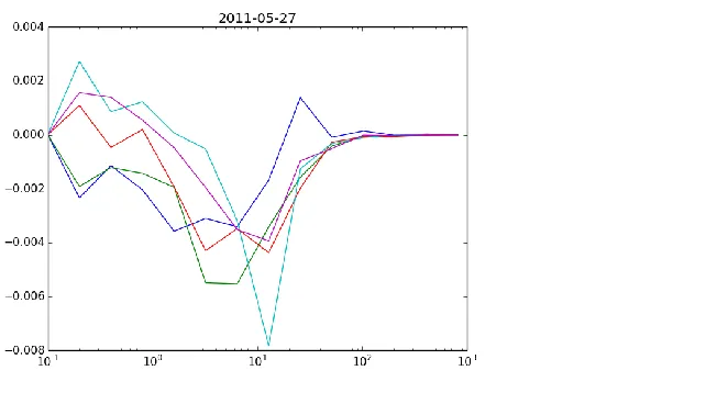
Figure 2.3 and 2.4 show the MRD calculated for the two test case days, using

data from top anemometers and beginning the calculation one hour after sunset. In Figure

2.3 the gap is identified as 18.56 seconds. This is the average peak from all five hour

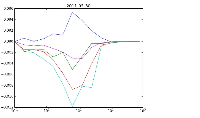
segments for the evening. Figure 2.4 show a longer gap of 53.76 seconds for the second

day, May 30, 2011. Each colored line on the graph represents thirty minutes of wind

data. The y-axis is the total heat flux cospectra calculated for each time scale. Heat flux,

measure of vertical motion in the atmosphere. Vertical motion in an atmosphere is also

another way to think of energy in the atmosphere. It takes energy for air to rise vertically.

The x-axis is a time scale measurement on a log scaled axis. The time scale is simply

saying that that is the amount of time that it took for an event (eddy) to pass the tower

and its associated sonic anemometer. The amount of time essentially is an indicator to the

size of an event, and therefore, how much energy the event is possibly holding or moving

throughout our forest. These events, especially the ones that occur in the aforementioned

gap are affecting the natural fluxes in a forest on a day-to-day basis.

Figure 2.4: The multi-resolutional decomposition found the gap on May 30, 2011 from 1800-2100. The average of all 5 hours is 53.76 seconds.

The differences between these two gaps can be accounted for by looking at the

average wind speed for those two time frames. The average wind speed for May 27, 2011

was slightly higher than the average wind speed for May 30, 2011, confirming that a

different gap scale is needed in the same environment based on difference timeframes.

On May 30, 2011, one of the lines also appears to have a heat flux in the opposite

directions. This is the first of the 30 minute averages, and although the heat flux is in the

opposite directions (possibly due to the sun still setting/ radiation differences) the gap

that is found using the MRD will not be affected because it is taking the average of all of

the gaps found and the gap appears to be on the same time frame as the other 30 minute

D. IDENTIFYING TREE MOTION

Like all physical structures, trees have a natural mode of frequency and are

susceptible to resonant loading. Therefore, understanding their periodic motion is

fundamental to understanding the absorption and dissipation of wind energy (Rudnicki et

al, 2008). Several studies have combined spectra from measurements of wind gusts with

spectra characterizing tree sway in order to construct mechanical transfer functions.

These types of studies reveal that wind gusts at or near the tree’s natural sway frequency

are efficiently transformed into tree motion and may induce resonance (Gardiner 1992;

White et al.1976).

The Fourier transform method takes advantage of the fact that continuous signals

can be decomposed to a sum of weighted sinusoidal functions. A Fast Fourier Transform

(FFT) can be applied to each tree to detect the fundamental mode of frequency over the

course of a particular time period. In previous studies the dominant frequency from each

Fourier transformed data segment were identified by applying a cutoff of any frequency

below 0.2 Hz and then automatically selecting the frequency with the highest power. The

resulting frequencies are assumed to represent the fundamental mode of tree vibration. In

this study an FFT was performed for each time segment identified by the MRD. That is

for every 18.5 seconds of tree data for the first day that was picked a single FFT was

computed. The frequency with the highest power was taken as the tree vibration due to

turbulence. This process effectively creates a time series of frequency values for each

In previous studies (Rudnicki et al. 2008), smoothing functions were used to find

an interpretable result. In Rudnicki’s study (2008) a Daniell filter was used for all of the

trees to minimize leakage and retain detail (Bloomfield 2000). A Daniell filter is a

smoothing process for displacement data, which helps to identify fundamental

frequencies. However, while the Daniell filter was useful for spectral loss, when

applying it to the sway data in this experiment, small changes in frequency from time step

to time step were lost. This is likely because of the short time periods that are being

examined in this experiment. Because this study is not only examining the fundamental

frequencies of the trees, but rather the changes in frequency, the Daniell filter was not

used. Instead a simple 5-point moving averaged was applied to the fourier power spectra

to aid in automated identification of the fundamental frequency in each time step. All

time series calculations, including the MRD and FFT were made using Python version

2.6 on a desktop PC. All the code can be found in Appendix A.

E. DYNAMIC MAPPING

In order to visualize how the fundamental frequency of each individual tree was

changing over time, the change in frequency was mapped and categorized based on either

an increase or a decrease in frequency. The study area was plotted according to exact

latitude and longitude coordinates into a layer in ArcMap. The frequency data was

imported into ESRI’s ArcMap and “joined” to the tree layer based on the tree id number,

Once the data was geolocated a spatial interpolation was preformed for each time step

(every 18.56 seconds for the first day and every 53.76 seconds for the second day). This

turns the 149 individual time series of frequency changes into a series of maps. The

analysis was done by batching all of the information for each tree and time period

together and running the Natural Neighbor interpolation to give a complete picture of the

entire data area.

The Natural Neighbor method is a geometric estimation technique that uses

natural neighborhood regions generated around each point in the data set. Like the

inverse distance weighting (IDW), this interpolation method is a weighted-average

interpolation method. However, instead of finding an interpolated point's value using all

of the input points weighted by their distance, Natural Neighbors interpolation creates a

Delauney Triangulation of the input points and selects the closest nodes that form a

convex hull around the interpolation point. It then “weighs” their values by proportionate

area. This method is most appropriate where sample data points are distributed with

uneven density. It is a good general-purpose interpolation technique and has the

advantage that you do not have to specify parameters such as radius, number of neighbors

or weights. This technique is designed to honor local minimum and maximum values in

the point file and can be set to limit overshoots of local high values and undershoots of

local low values. The method thereby allows the creation of accurate surface models from

C

3:

R

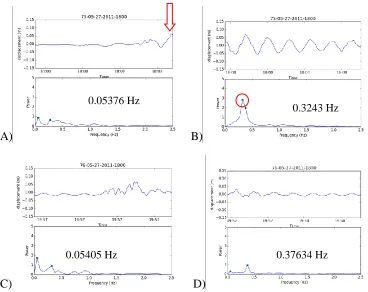
Figure 3.1 shows an example of the process of converting tree displacement to

changes in frequency. The figure shows the raw time signal and the FFT for trees # 75

and #76. Both are located near the center of the plot. By looking at the figure it can be

observed that the chosen time scale for this particular night finds a change in for the onset

and offset of gusts.

A) B)

C) D)

Figure 3.1: FFT Results May 27, 2011 -- The purpose of comparing these two variables is to identify the onset of a gust in the forest (indicated by the arrow in Figure 3.1A) and then observe what happens to the peak frequency of that time frame(circled in Figure 3.1B) when the displacement is changing. Each top panel shows the displacement over a

period of time. The bottom panels show the corresponding frequency change (power)— 0.05376 Hz

0.3243 Hz

both on the x-axis. The peak frequency in the lower panel is denoted by a dot. The change in this peak frequency is the mapable variable for the animations. A&B Tree 75 from

18:00:00.01 to 18:00:37.22 C&D Tree 76 from 19:57:00.01 50 19:57:37.22

Figure 3.1 clearly indicated that there is a change in the tree’s peak frequency

upon the arrival of a gust. In Figures 3.1A and 3.1B it can be observed that the peak

frequency of the tree is increased from 0.05Hz to 0.32Hz with the onset and occurrence

of a gust. The same is true in Figures 3.1C and 3.1D, which show the tree movement and

frequency for a time later in the evening. Here the frequency changes from its resting

level of 0.05Hz to a movement frequency of 0.37Hz. This indicates that a positive change

in frequency is a good parameter for the identification of a gust affecting a tree in the

forest. This was further analyzed to see if the apparent increase in the fundamental

frequency does not just occur in one place, at one tree, but rather in groups, which can be

identified throughout the study area.

In order to identify coherency at the MRD calculated time step, the FFT was also

performed at another record length, which is double that of the spectral gap calculated

using MRD. This was done as a control comparison. For May 27, 2011 this was a record

length of 37 seconds and for May 30, 2011 a record length of 106 seconds was used. The

output of the longer time FFT was also mapped using the same steps mentioned above.

Figure 3.2 shows the results for the same starting time presented in Figure 3.1. Thus, the

left panels of Figure 3.2 show the combined time series of panels A&B of Figure 3.1 and

the right panel shows the next 106 seconds. When the record time is doubled the figures

of a gust (Webb et al, 1980), like the gap scale figures previously showed. This was true

for the majority of the plots at the longer time length.

Figure 3.2: FFT Results May 27, 2011—double record length. The left panel shows the combined time series of the top panels of Figure 3.1 and the right panel shows the combined time series of the bottom panels of Figure 3.1. Tree 75 is from 18:00:00.01 to

18:00:37.22 and Tree 76 is from 19:57:00.01 50 19:57:37.22. As the Red circles indicate, there is no detection of a peak frequency in these examples.

Because the main goal of this thesis was to determine coherency in the data, only

a subset of each night was mapped for visual aid. For each night the first 30 minutes of

data was compiled into an animated map. This captures the occurrence of a moderate to

high wind speed on each day, which as previously discussed, should yield more apparent

gusts. Viewing of the animations, revealed an interesting picture of the forest. The

animations are attached on an included CD. Static images from the animations are shown

below for discussion. In all of the maps, shades of blue represent a decreasing change in

frequency from the previous time step and the shades of red indicate an increase in

frequency.

When observing the animations the movement of the gusts through the forest site

becomes more apparent—particularly at the gap time scale. As shown in the static

images, there are some instances in the time frame that I examined where a gust

impression was apparent and a gust moved through the site, but it only appeared at the

gap time scale animation and was completely missed, or virtually non-existent in the

longer time step animation. The color changes between a decrease in frequency (blue)

and an increase in frequency (reds) are usually very well coordinated—if there was a

major increase as a gust moved through a section of a forest in one frame in the next

frame there is a corresponding decrease in frequency as the tree begins to return back to

its natural frequency. Overall movement in the animations corresponds with the wind

direction observed by the central tower on the research site.

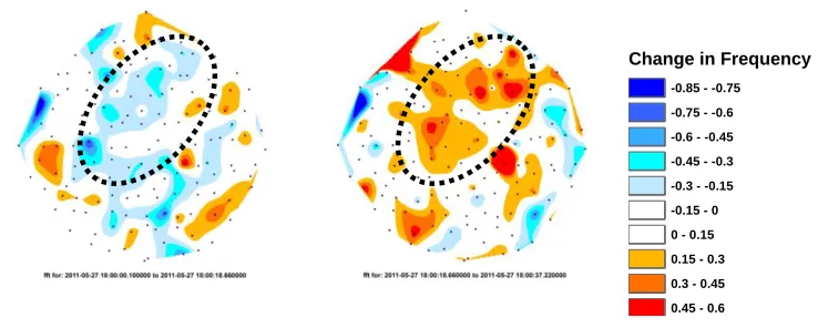
Figure 3.3: Static images of the frequency changes occurring from 2011-05-27 18:00:00.01 to 18:00:37.22 at the gap time scale. During this time wind direction was predominantly from the northwest. Each image represents the frequency found from an

18 second record

Change in Frequency

-0.85 - -0.75

-0.75 - -0.6 -0.6 - -0.45

-0.45 - -0.3

-0.3 - -0.15 -0.15 - 0

0 - 0.15 0.15 - 0.3

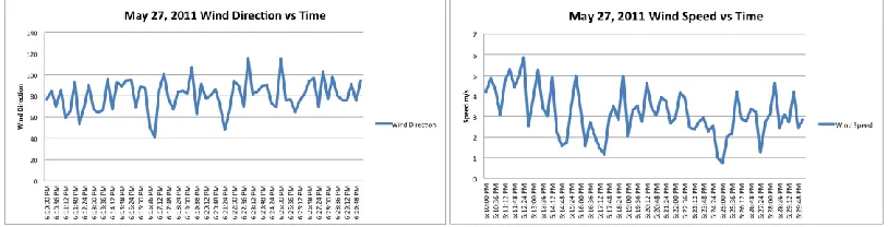
Figure 3.4: Plots of the Wind Direction and Wind Speed corresponding with the time periods looked at in the attached animations.

Figure 3.5: Static image of the frequency changes occurring from 2011-05-27 18:00:00.01 to 18:00:37.22 at double the gap time scale.

Figure 3.3 shows results from May 27th when computing frequency changes at the

gap-scale. In the first image, a predominant decrease in frequency is seen through the

center of the plot (highlighted with the dashed circle), with some areas of increase on the

outer edges. In the second image a predominant increase in frequency is seen—which can

be attributed to a response to the previous decrease in the time step before. This

momentary decrease is interpreted as a gust moving the canopy. The wind speed shown

in Figure 3.4 confirms this. Figure 3.5 shows the results of the computed frequency

Change in Frequency

-0.85 - -0.75

-0.75 - -0.6

-0.6 - -0.45 -0.45 - -0.3

-0.3 - -0.15 -0.15 - 0

0 - 0.15 0.15 - 0.3

changes at double the gap-scale on May 27th, 2011. The absence of any frequency

increase or decrease indicates that the frequency changes are lost when computing

frequency at times longer than the gap-scale. The decrease and subsequent increase in

frequency would not have been detected and instead, the data would have just showed an

overall decrease between those two time steps. Essentially, the tree’s response to the gust

occurring at the time is lost, and the bounce back, return to normalcy, or increase in

frequency is not detected at double the gap scale.

A second example from May 27th is shown in Figure 3.6 below.

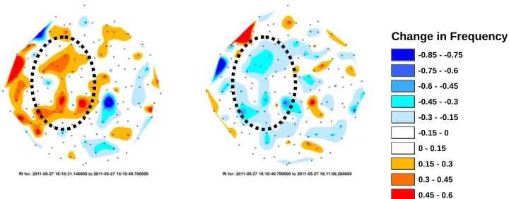
Figure 3.6: Static images of the frequency changes occurring from 2011-05-27 18:10:31.14 to 18:11:08.26 at the gap time scale

Change in Frequency

-0.85 - -0.75

-0.75 - -0.6 -0.6 - -0.45

-0.45 - -0.3 -0.3 - -0.15

-0.15 - 0 0 - 0.15

0.15 - 0.3

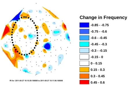
Figure 3.7: Static image of the frequency change occurring from 2011-05-27 18:10:29.14 to 18:11:06.26 at double the gap time scale

In the first two images above, there is an apparent gust impression occurring

between the time steps of 18:10:31.14- 18:10:49.7 and 18:10:49:7- 18:11:08:26, however

no gust is identifiable in Figure 3.7, which shows the computed frequency change when

using double the gap-scale for the computation window. This is expected and apparent

because of the theory proposed above that the gusts and coherent motions will be more

visible at a time scale that is determined by MRD, rather than an averaged time scale for

the entire study time.

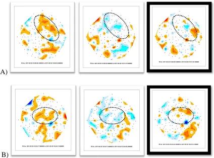
On the night of May 30th, the wind speed was 2.4m/s and the gap-scale was longer

(53.76 seconds). Overall the results are similar with more coherency and subtle changes

in tree motion seen when using the proposed gap-scale as a window-length versus a

longer period. Figure 3.8 below shows several static images from this night. These

images are interesting because even though the average wind speed for this night was

slightly slower than the previous date chosen, coherent motions can still clearly be seen at

Change in Frequency

-0.85 - -0.75

-0.75 - -0.6 -0.6 - -0.45

-0.45 - -0.3 -0.3 - -0.15

-0.15 - 0

0 - 0.15 0.15 - 0.3

the gap scale and are completely overlooked at the double time step (highlighted with

dashed circle). This indicates that choosing an appropriate time scale for these gusts is

even more important when the wind speed is not as high.

A)

B)

Figure 3.8: (A) Static images of the frequency changes occurring from 2011-05-30 18:00:00.01 to 18:01:47.62 at the gap time scale with the outlined image showing the

same time frame, but double the gap time scale (B) Static images of the frequency changes occurring from 2011-05-30 18:23:17.86 to 18:25:05.38 at the gap time scale

C

4:

D

/

C

The results presented in chapter three confirm the original hypothesis that

coherent motions in a forest canopy are occurring on turbulent time scales. Less

coherence is seen when examining motion on time scales greater than the co-spectral gap,

which would include meso and sub meso scale motions. This further proves that

identifying the importance of a time scale is imperative to predicting the response of trees

in a forest environment. In this particular case, frequency proved to be a good variable for

mapping the wind and capturing the occurrence of the small-scale gusts. Overall this

work highlights how helpful dynamic maps can be for displaying rapidly changing spatial

patterns. As a preliminary analysis this work also highlights a number of other future

research directions.

Several aspects of this study could be improved in the future. When looking back

at the mapping outputs, a particular tree is always highlighted. After looking more into

the specifics of this tree it is clear that it is much bigger than the surrounding trees, hence

causing the FFT to highlight it more often. This could also have something to do with the

method of peak detection algorithm that was chosen—another method might have been

better or more accurate. Also, more standardization of the data might have prevented this.

Also, because of the limitations of this study, only two days out of several years of data

were used. Expanding the time frame would have given us a better look at the differences

remains unclear as to whether this method will work for moderate wind speed days, when

the changes in frequency are not as noticeable, as only days with high winds speeds were

chosen for this particular study.

The animations that were created for this project were a great start, but there

needs to be more flexibility in controlling the time step as well as the time frame that can

be looked at. If the time step could be customized and changed to start later in the time

frame it would ensure that any gust, at any point in the forest can be captured. This means

that you could track the movement of a gust from its entrance to the research site until it

exits—still using the gap scale. If a tool like this could be created, it would help to apply

these findings to other areas, not just forests so that researchers can get an idea of how

small-scale winds interact on a variety of different terrains.

The more immediate take away from this study pertains to the specific field of

micrometeorology and forestry. Now that I have proved that there is coherency occurring

in the boundary layer at particular time scales, the next step is to figure out what can

define this coherency and how to move forward into defining exactly what constitutes as

spatial correlation, i.e. a certain number of trees moving in the same direction, etc.

Identifying areas that are spatially correlated would help in forestry management/damage

predictions.

There has long been an underlying assumption in meteorology that sub synoptic-scale

phenomena such as turbulence might be responsible for the difficulty in making quality

meteorology involves the search for accurate turbulence parameterization schemes for

larger-scale numerical forecast models. Progress made from this project will build a

foundation, in both field experimental design and numerical model development, for

pursuing investigations of these interactions in more complex situations in the near

R

Amiro, B. D. “Comparison of Turbulence Statistics Within Three Boreal Forest Canopies.” Boundary-Layer Meteorology 51, no. 1–2 (April 1, 1990): 99–121. doi:10.1007/BF00120463.

Baker, C.J. “The Development of a Theoretical Model for the Windthrow of Plants.”

Journal of Theoretical Biology 175, no. 3 (August 7, 1995): 355–372.

doi:10.1006/jtbi.1995.0147.

Baldocchi, D. D. & Hutchinson, B. A. 1987 Turbulence in an almond orchard: vertical variation in turbulence statistics. Boundary-Layer Meteorol. 40, 177–146.

Baldocchi, Dennis D., and Tilden P. Meyers. “Turbulence Structure in a Deciduous Forest.” Boundary-Layer Meteorology 43, no. 4 (June 1, 1988): 345–364. doi:10.1007/BF00121712.

Banta, R., R. Newsom, J. Lundquist, Y. L. Pichugina, R. L. Coulter,and L. Mahrt, 2002: Nocturnal low-level jet characteristics over Kansas during CASES-99.Bound.-Layer Meteor., 105, 221–252.

Bloomfield P (2000) Fourier analysis of time series: an introduction. Wiley, New York

Bohm, M., Finnigan, J. J. & Raupach, M. R. 2000 Dispersive fluxes and canopy flows: just how important are they? In Proceedings of 24th Conference on Agricultural and Forest Meteorology, American Meteorological Society, Davis, CA.

Boose, Emery R., David R. Foster, and Marcheterre Fluet. “Hurricane Impacts to Tropical and Temperate Forest Landscapes.” Ecological Monographs 64, no. 4 (November 1994): 369. doi:10.2307/2937142.

Brunet, Y., J. J. Finnigan, and M. R. Raupach. “A Wind Tunnel Study of Air Flow in Waving Wheat: Single-point Velocity Statistics.” Boundary-Layer Meteorology 70, no. 1–2 (July 1, 1994): 95–132. doi:10.1007/BF00712525.

Businger, J. A., J. C. Wyngaard, Y. zumi, and E. F. Bradley, 1971:Flux profile relationships in the atmospheric surface layer. J.Atmos. Sci., 28, 181–189.

Canham and Loucks 1984 Ecol 65 803 809 Pdf Free Ebook Download. Accessed April

Cellier, P., and Y. Brunet. “Flux-gradient Relationships Above Tall Plant Canopies.”

Agricultural and Forest Meteorology 58, no. 1–2 (March 1992): 93–117.

doi:10.1016/0168-1923(92)90113-I.

Colorado, Atmospheric Studies Program Area J. C. Kaimal Chief, Wave Propagation Laboratory Environmental Research Laboratories National Oceanic and Atmospheric Administration Boulder, and Center for Environmental Mechanics J. J. Finnigan Head, Australia National Oceanic and Atmospheric Administration Boulder Colorado.

Atmospheric Boundary Layer Flows : Their Structure and Measurement: Their

Structure and Measurement. Oxford University Press, 1993.

Dale, V. H., L. A. Joyce, S. McNulty, R. P. Neilson, M. P. Ayres, M. D. Flannigan, P. J. Hanson, et al. Climate Change and Forest Disturbances, 2001.

http://www.treesearch.fs.fed.us/pubs/30125.

David Foster, and Emery R. Boose. “Patterns of Forest Damage Resulting from Catastrophic Wind in Central New England, USA” (n.d.).

Dyer, A., 1974: A review of flux-profile relationships. Bound.-Layer Meteor., 7, 363– 372.

Dwyer, M. J., Patton, E. G. & Shaw, R. H. 1997 Turbulent kinetic energy budgets from a large-eddy simulation of airflow above and within a forest. Boundary-Layer Meteorol. 84,23–43.

Emanuel, Kerry. “Increasing Destructiveness of Tropical Cyclones over the Past 30 Years.” Nature 436, no. 7051 (August 4, 2005): 686–688.

doi:10.1038/nature03906.

Finnigan 2000 Annual Review Fluid Mech Pdf Free Ebook Download. Accessed April 8,

2013. http://ebookbrowse.com/finnigan-2000-annual-review-fluid-mech-pdf-d131921957.

Finnigan, John. “Turbulence in Plant Canopies.” Annual Review of Fluid Mechanics 32, no. 1 (2000): 519–571. doi:10.1146/annurev.fluid.32.1.519

———. “Turbulence in Plant Canopies.” Annual Review of Fluid Mechanics 32, no. 1 (2000): 519–571. doi:10.1146/annurev.fluid.32.1.519.

Gao, W., R. H. Shaw, and K. T. Paw U. “Observation of Organized Structure in

Turbulent Flow Within and Above a Forest Canopy.” In Boundary Layer Studies and

Applications, edited by R. E. Munn, 349–377. Springer Netherlands, 1989.

Gardiner B (1992) Mathematical modelling of the static and dynamic characteristics of plantation trees. In: Franke J, Roeder A (eds) Mathematical modelling of forest ecosystems. Sauerlander, Frankfurt, pp 40–61

Gardiner, B. A. “Wind and Wind Forces in a Plantation Spruce Forest.” Boundary-Layer

Meteorology 67, no. 1–2 (January 1, 1994): 161–186. doi:10.1007/BF00705512.

Henry, Hugh A. L., and Sean C. Thomas. “Interactive Effects of Lateral Shade and Wind on Stem Allometry, Biomass Allocation, and Mechanical Stability in Abutilon

Theophrasti (Malvaceae).” American Journal of Botany 89, no. 10 (October 1, 2002): 1609–1615. doi:10.3732/ajb.89.10.1609.

Howell, J. F., and L. Mahrt, 1997: Multiresolution flux decomposition.Bound.-Layer Meteor., 83, 117–137

Irvine, M. R., B. A. Gardiner, and M. K. Hill. “The Evolution Of Turbulence Across A Forest Edge.” Boundary-Layer Meteorology 84, no. 3 (September 1, 1997): 467–496. doi:10.1023/A:1000453031036.

James, Kenneth R, Nicholas Haritos, and Peter K Ades. “Mechanical Stability of Trees Under Dynamic Loads.” American Journal of Botany 93, no. 10 (October 2006): 1522–1530. doi:10.3732/ajb.93.10.1522.

Kaimal, J. C., and J. J. Finnigan, 1994: Atmospheric Boundary Layer Flows: Their Structure and Measurements. Oxford University Press, 289 pp.

Katul, G G, A Porporato, R Nathan, M Siqueira, M B Soons, D Poggi, H S Horn, and S A Levin. “Mechanistic Analytical Models for Long-distance Seed Dispersal by Wind.”

The American Naturalist 166, no. 3 (September 2005): 368–381. doi:10.1086/432589.

Katul, G., and B. Vidakovic, 1996: The partitioning of attached and detached eddy motion in the atmospheric surface layer using Lorentz wavelet filtering. Bound.-Layer Meteor., 77, 153–172.

Law, Beverly. “Carbon Dynamics in Response to Climate and Disturbance: Recent Progress from Multi-scale Measurements and Modeling in AmeriFlux” (n.d.).

Mahrt, L., 1998: Flux sampling strategy for aircraft and tower observations. J. Atmos. And Oceanic Technol., 15, 416-429.

Marshall, B. J., C. J. Wood, B. A. Gardiner, and R. E. Belcher. “Conditional Sampling Of Forest Canopy Gusts.” Boundary-Layer Meteorology 102, no. 2 (February 1, 2002): 225–251. doi:10.1023/A:1013181714844.