Two modified least squares iterative algorithms for the Lyapunov matrix equations

(1)

R E S E A R C H

Open Access

Two modiﬁed least-squares iterative

algorithms for the Lyapunov matrix equations

Min Sun

1*

_{, Yiju Wang}

2

_{and Jing Liu}

3

*_{Correspondence:} [email protected] 1_{School of Mathematics and}

Statistics, Zaozhuang University, Shandong, P.R. China Full list of author information is available at the end of the article

Abstract

In this paper two modified least-squares iterative algorithms are presented for solving the Lyapunov matrix equations. The first algorithm is based on the hierarchical identification principle, which can be viewed as a surrogate of the least-squares iterative algorithm proposed by Ding et al., whose convergence has not been proved until now. The second one is motivated by a new form of fixed point iterative scheme. With the tool of a new matrix norm, the proof of both algorithms’ global convergence is offered. Furthermore, the feasible sets of their convergence factors are analyzed. Finally, a numerical example is presented to illustrate the rationality of theoretical results.

MSC: 65H10; 90C33; 90C30

Keywords: Least-squares iterative algorithm; Lyapunov matrix equations; Hierarchical identiﬁcation principle

1 Introduction

Matrix equations are often encountered in control theory [1,2], system theory [3,4], and stability analysis [5–7]. For example, the stability of the autonomous systemx˙(t) =Ax(t) is determined by whether the associated Lyapunov equationXA+AX= –Mhas a positive deﬁnite solutionX, whereMis a given positive deﬁnite matrix with approximate size [8]. In this paper, we are concerned with the following (continuous-time) Lyapunov matrix equations:

AX+XA=C, (1.1)

whereA∈Rm×m andC∈Rm×m are the given constant matrices, andX∈Rm×m is the unknown matrix to be determined.

Obviously, by using the Kronecker product⊗and the vec-operatorvec, equation (1.1) can be written as a system of linear equations:

(Im⊗A+A⊗Im)vec(X) =vec(C). (1.2)

The order of its coeﬃcient matrix ism2, which becomes very large when the constant

mis large. For example, ifm= 100, thenm2_{= 10, 000. Obviously, a 10,000 order square}

(2)

matrix requires much more storage capacity than several 100 order square matrices. Fur-thermore, the inverse computation and eigenvalue computation of 10,000 order square matrix are much more diﬃcult than those of 100 order square matrix.

To solve equation (1.1) or its special cases or generalized versions, different methods have been developed in the literature [5,7,9–19], which belong to the category of itera-tive methods. For example, two conjugate gradient methods are proposed in [7] to solve consistent or inconsistent equation (1.1). Both have finite termination property in the ab-sence of round-off errors and can get least Frobenius norm solution or least-squares solu-tion with the least Frobenius norm of equasolu-tion (1.1) when they adopt some special kind of initial matrix. By using the hierarchical identification principle, Ding et al. [18] designed a gradient-based iterative algorithm and a least-squares iterative algorithm for equation (1.1), and they proved that the gradient-based iterative algorithm always converges to the exact solution for any initial matrix. However, convergence of the least-squares iterative algorithm is not proved in [18]. In fact, the authors claimed that convergence of the least-squares iterative algorithm is very difficult to prove and still requires studying further. In this paper, we are going to further study the least-squares iterative algorithm for equa-tion (1.1) and present two convergent least-squares iterative algorithms. The feasible set of their convergence factor is presented.

The remainder of the paper is organized as follows. Section2presents the ﬁrst least-squares iterative algorithm for equation (1.1) and its global convergence. Section3 dis-cusses the second least-squares iterative algorithm for equation (1.1) and its global con-vergence. Section4gives an example to illustrate the rationality of theoretical results. Sec-tion5ends the paper with some remarks.

2 The ﬁrst algorithm and its convergence

In this section, we give some notations, present the ﬁrst least-squares iterative algorithm for equation (1.1), and analyze its global convergence.

The symbolIstands for an identity matrix of approximate size. For anyM∈Rn×n, the symbolλmax[M] denotes the maximum eigenvalue of the square matrixM. For anyN∈

Rm×n_{, we use}_N_{to denote its transpose, and the symbol tr(}_N_{) to stand for its trace. The} Frobenius normNis defined asN=tr(NN). The symbolA⊗Bdefined asA⊗B= (aijB) stands for the Kronecker product of matricesAandB. For a matrixA∈Rm×n, the vectorization operatorvec(A) is defined byvec(A) = (a₁,a₂, . . . ,a_n), whereakis thekth column of the matrix A. According to the property of the Kronecker product, for any matricesM,N, andXwith approximate size, we have

vec(MXN) =N⊗Mvec(X).

The following deﬁnition is a simple extension of the Frobenius norm · .

Deﬁnition 2.1 Given a positive deﬁnite matrixM∈Rn×nand a matrixN∈Rm×n, the

M-Frobenius normNMis deﬁned as

NM=

trNMN. (2.1)

(3)

Theorem 2.1 Given a positive deﬁnite matrix M∈Rn×nand three matrices N,N1,N2∈

Rm×n_,_{it holds that}

(1) NM= 0⇐⇒N= 0.

(2) N1+N22M=N1M2 + 2tr(N1MN2) +N22M.

Proof The proof is elementary and is omitted here.

Theorem 2.2([18]) Equation(1.1)has a unique solution if and only if the matrix Im⊗

A+A⊗Imis nonsingular,and the unique solution X∗is given by

vecX∗= [Im⊗A+A⊗Im]–1vec(C).

By using the hierarchical identiﬁcation principle, Ding et al. [18] presented the following least-squares iterative algorithm for equation (1.1):

X1(k) =X(k– 1) +μ

The following example shows that the feasible set of the convergence factorμof iterative scheme (2.2)–(2.4) maybe not the interval (0, 4).

Example2.1 Consider the Lyapunov matrix equationsAX+XA=Cwith

A=

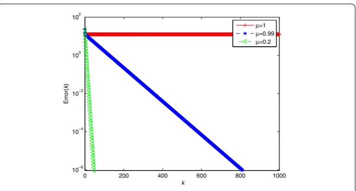
The numerical results of iterative scheme (2.2)–(2.4) withμ= 1, 0.99, 0.2 are plotted in Fig.1, in which

Error(k) =AX(k) +X(k)A–C.

From the three curves in Fig.1, we ﬁnd that: (1) iterative scheme (2.2)–(2.4) withμ= 1 is divergent, while iterative scheme (2.2)–(2.4) withμ= 0.99, 0.2 is convergent; (2) the constant 1 maybe the upper bound ofμfor this example; (3) smaller convergence factor often can accelerate the convergence of iterative scheme (2.2)–(2.4).

(4)

Figure 1Numerical results of iterative scheme (2.2)–(2.4) with diﬀerentμ

Remark2.1 Modiﬁed least-squares iterative algorithm (2.2), (2.5), and (2.6) involves the inverse of the matrixAA. However, since this term is invariant in each iteration, we need only compute it once before all iterations.

In the remainder of this section, we shall prove the global convergence of the ﬁrst least-squares iterative algorithm (2.2), (2.5), and (2.6), which is motivated by Theorem 4 in [18].

Theorem 2.3 If equation(1.1)has a unique solution X∗and r(A) =m,the sequence{X(k)}

generated by iterative scheme(2.2), (2.5),and(2.6)converges to X∗ for any initial matrix X(0),where the convergence factorμsatisﬁes

0 <μ<2

ν, (2.7)

and the constantνis deﬁned as

ν= 1 +λmax

AAλmax

AA–1.

Proof Firstly, let us deﬁne three error matrices as follows:

˜

X1(k) =X1(k) –X∗,

AA–1/2X˜2(k) =X2(k) –X∗, X˜(k) =X(k) –X∗.

Then, by (2.4), the error matrix corresponding toX(k) can be written as

˜

X(k) =X1(k) +X2(k)

2 –X

∗₌X˜1(k) +X˜2(k)

2 . (2.8)

Thus, from the convexity of the function · 2_A_A, it holds that

X˜(k)2_A_A≤

˜X1(k)2_A_A+ ˜X2(k)2_A_A

2 =

˜X1(k)2_A_A+ ˜X2(k)2_A_A

(5)

Secondly, setting

Similarly, from (2.12) and Theorem2.1, we have

X˜2(k)

Substituting the above two inequalities into the right-hand side of (2.9) yields

(6)

from which it holds that

lim

k→∞

ξ(k) +η(k)= 0.

That is,

lim

k→∞

AX˜(k– 1) +X˜(k– 1)A= 0.

So

lim

k→∞[Im⊗A+A⊗Im]vec

_˜

X(k– 1)= 0.

Since the matrixIm⊗A+A⊗Imis nonsingular, we have

lim

k→∞vec

_˜

X(k– 1)= 0.

Thus

lim

k→∞X(k) =X ∗_.

This completes the proof.

Remark2.2 We can adopt some iterative methods, such as the sum method, the power method [20], to compute the maximum eigenvalue in the constantν.

3 The second algorithm and its convergence

In this section, we present the second least-squares iterative algorithm for equation (1.1) and analyze its global convergence.

Deﬁne a matrixC¯ as follows:

¯

C=C–XA. (3.1)

Then equation (1.1) can be written as

S:AX=C¯.

From [18], the least-squares solution of the systemSis

X=AA–1AC¯.

Substituting (3.1) into the above equation, we have

X=AA–1AC–XA.

Then, we get the second least-squares iterative algorithm for equation (1.1) as follows:

X(k) =X(k– 1) –μX(k– 1) –AA–1AC–X(k– 1)A. (3.2)

(7)

Theorem 3.1 If equation(1.1)has a unique solution X∗and r(A) =m,the sequence{X(k)}

generated by iterative scheme(3.2)converges to X∗for any initial matrix X(0),where the convergence factorμsatisﬁes

0 <μ< 2 + 2λmin(A⊗A

–1₎

1 +λ2

max(A⊗A–1) + 2λmin(A⊗A–1)

. (3.3)

Proof Firstly, let us deﬁne an error matrix as follows:

˜

X(k) =X(k) –X∗.

Then, by (3.2), it holds that ˜

X(k) =X(k) –X∗

=X(k– 1) –X∗–μX(k– 1) –AA–1AC–X(k– 1)A

=X˜(k– 1) –μX(k– 1) –AA–1AAX∗+X∗A–X(k– 1)A

= (1 –μ)X˜(k– 1) +μAA–1AX∗A–X(k– 1)A

= (1 –μ)X˜(k– 1) +μA–1X∗–X(k– 1)A

= (1 –μ)X˜(k– 1) –μA–1X˜(k– 1)A.

So

vecX˜(k)= (1 –μ)vecX˜(k– 1)–μA⊗A–1vecX˜(k– 1).

Then

vecX˜(k)2

= (1 –μ)2vecX˜(k– 1)2– 2μ(1 –μ)vecX˜(k– 1)A⊗A–1vecX˜(k– 1)

+μ2A⊗A–1vecX˜(k– 1)2

≤1 + 2μ+μ2– 2μ(1 –μ)λmin

A⊗A–1+μ2λ2_maxA⊗A–1vecX˜(k– 1)2.

Setν= 1 + 2μ+μ2_{– 2}_μ_{(1 –}_μ₎_λ

min(A⊗A–1) +μ2λ2max(A⊗A–1). From (3.3), it holds that

0 <ν< 1. Thus

vecX˜(k)2≤νvecX˜(k– 1)2≤νkvecX˜(0)2.

Then

lim

k→∞vec

_˜

X(k)= 0.

So

lim

k→∞X(k) =X ∗_.

(8)

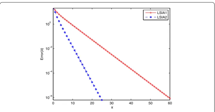
Figure 2Numerical results of the two tested algorithms (LSIA1 and LSIA2)

Example3.1 Let us apply the two modiﬁed least-squares iterative algorithms, i.e., iterative scheme (2.2), (2.5), and (2.6) (denoted by LSIA1) and iterative scheme (3.2) (denoted by LSIA2), to solve the Lyapunov matrix equations in Example2.1. We setμ= 0.2546 in the ﬁrst algorithm andμ= 0.3478 in the second algorithm. The numerical results are plotted in Fig.2.

The two curves in Fig.2 illustrate that the two modiﬁed least-squares iterative algo-rithms are both convergent, and LSIA2 is faster than LSIA1 for this problem.

4 Numerical results

In this section, an example is given to show the eﬃciency of the two proposed algorithms (denoted by LSIA1 and LSIA2) in Sect.2and Sect.3, and we give some comparisons with the gradient-based iterative algorithm in [18] (denoted by GBIA). The convergence factors in both algorithms are set to their upper bounds.

Example4.1 Let us consider a medium scale Lyapunov matrix equation

AX+XA=C,

with

A= –triurand(n), 1+diag8 –diagrand(n), C=rand(n).

We setn= 20 and set the initial matrixX(0) = 0.

(9)

Figure 3Numerical results of LSIA1, LSIA2, and GBIA

5 Conclusions

In this paper, two modiﬁed least-squares iteration algorithms are proposed for solving the Lyapunov matrix equations, whose global convergence is proved. The feasible set of their convergence factor is analyzed. Some numerical results are presented to verify the theoretical results. In the future, we shall analyze the convergence property of the least-squares iteration algorithm for solving the Sylvester matrix equations.

Acknowledgements

The authors thank two anonymous reviewers for their valuable comments and suggestions that have helped them in improving the paper.

Funding

This work is supported by the National Natural Science Foundation of Shandong Province (No. ZR2016AL05) and the Doctoral Foundation of Zaozhuang University.

Competing interests

The authors declare that there are no competing interests.

Authors’ contributions

The first author provided the problem and gave the proof of the main results, the second author finished the numerical experiment, and the third author improved the writing. All authors read and approved the final manuscript.

Author details

1_{School of Mathematics and Statistics, Zaozhuang University, Shandong, P.R. China.}2_{School of Management Science,}

Qufu Normal University, Rizhao, P.R. China. 3_{School of Data Sciences, Zhejiang University of Finance and Economics,}

Zhejiang, P.R. China.

Publisher’s Note

Springer Nature remains neutral with regard to jurisdictional claims in published maps and institutional aﬃliations.

Received: 21 April 2019 Accepted: 22 July 2019

References

1. Wu, A.G., Fu, Y.M., Duan, G.R.: On solutions of matrix equationsv–AVF=BWandv–aVf¯ =BW. Math. Comput. Model.

47(11–12), 1181–1197 (2008)

2. Wu, A.G., Wang, H.Q., Duan, G.R.: On matrix equationsx–AXF=candx–aXf¯ =c. J. Comput. Appl. Math.230(2), 690–698 (2009)

3. Zhang, H.M., Ding, F.: Iterative algorithms forx+ax–1_a₌_i_{by using the hierarchical identiﬁcation principle. J.}

Franklin Inst.353(5), 1132–1146 (2016)

(10)

5. Hajarian, M.: Developing biCOR and CORS methods for coupled Sylvester-transpose and periodic Sylvester matrix equations. Appl. Math. Model.39(9), 6073–6084 (2015)

6. Song, C.Q., Feng, J.E.: On solutions to the matrix equationsXB–AX=CYandXB–aXˆ=CY. J. Franklin Inst.353(5), 1075–1088 (2016)

7. Sun, M., Wang, Y.J.: The conjugate gradient methods for solving the generalized periodic Sylvester matrix equations. J. Appl. Math. Comput.60, 413–434 (2019)

8. Datta, B.N.: Numerical Methods for Linear Control Systems. Elsevier, Amsterdam (2003)

9. Ding, J., Liu, Y.J., Ding, F.: Iterative solutions to matrix equations of the formAiXBi=Fi. Comput. Math. Appl.59(11), 3500–3507 (2010)

10. Xie, L., Liu, Y.J., Yang, H.Z.: Gradient based and least squares based iterative algorithms for matrix equations AXB+CXD=F. Appl. Math. Comput.217(5), 2191–2199 (2010)

11. Ding, F., Chen, T.W.: Iterative least-squares solutions of coupled Sylvester matrix equations. Syst. Control Lett.54(2), 95–107 (2005)

12. Xie, L., Ding, J., Ding, F.: Gradient based iterative solutions for general linear matrix equations. Comput. Math. Appl.

58(7), 1441–1448 (2009)

13. Ding, F., Zhang, H.M.: Gradient-based iterative algorithm for a class of the coupled matrix equations related to control systems. IET Control Theory Appl.8(15), 1588–1595 (2014)

14. Ding, F., Chen, T.W.: On iterative solutions of general coupled matrix equations. SIAM J. Control Optim.44(6), 2269–2284 (2006)

15. Chen, L.J., Ma, C.F.: Developing CRS iterative methods for periodic Sylvester matrix equation. Adv. Diﬀer. Equ.2019, 87 (2019)

16. Berzig, M., Duan, X.F., Samet, B.: Positive deﬁnite solution of the matrix equationX=Q?A∗X?1_A₊_B∗_X?1_B_via

Bhaskar–Lakshmikantham ﬁxed point theorem. Adv. Diﬀer. Equ.627 (2012)

17. Vaezzadeh, S., Vaezpour, S.M., Saadati, R., Park, C.: The iterative methods for solving nonlinear matrix equation X+A∗X?1_A_+B∗_X?1_B₌_{Q. Adv. Diﬀer. Equ.}₂₀₁₃_{, 27 (2013)}

18. Ding, F., Liu, P.X., Ding, J.: Iterative solutions of the generalized Sylvester matrix equations by using the hierarchical identiﬁcation principle. Appl. Math. Comput.,197(1), 41–50 (2008)

19. Sun, M., Wang, Y.J., Liu, J.: Generalized Peaceman–Rachford splitting method for multiple-block separable convex programming with applications to robust PCA. Calcolo54(1), 77–94 (2017)