Extracting Vessel Structure From 3D Image Data

Scholarship@Western

Scholarship@Western

Electronic Thesis and Dissertation Repository

1-29-2014

Extracting Vessel Structure From 3D Image Data

Extracting Vessel Structure From 3D Image Data

Yuchen Zhong

The University of Western Ontario Supervisor

Yuri Boykov

The University of Western Ontario Graduate Program in Computer Science

A thesis submitted in partial fulfillment of the requirements for the degree in Master of Science © Yuchen Zhong 2014

Follow this and additional works at: https://ir.lib.uwo.ca/etd

Part of the Cardiovascular System Commons, Geometry and Topology Commons, Graphics and Human Computer Interfaces Commons, and the Other Computer Sciences Commons

Recommended Citation Recommended Citation

Zhong, Yuchen, "Extracting Vessel Structure From 3D Image Data" (2014). Electronic Thesis and Dissertation Repository. 1883.

https://ir.lib.uwo.ca/etd/1883

This Dissertation/Thesis is brought to you for free and open access by Scholarship@Western. It has been accepted for inclusion in Electronic Thesis and Dissertation Repository by an authorized administrator of

(Thesis format: Monograph)

by

Yuchen Zhong

Graduate Program in Computer Science

A thesis submitted in partial fulfillment

of the requirements for the degree of

Master of Science

The School of Graduate and Postdoctoral Studies

The University of Western Ontario

London, Ontario, Canada

c

This thesis is focused on extracting the structure of vessels from 3D cardiac images. In

many biomedical applications it is important to segment the vessels preserving their

anatomically-correct topological structure. That is, the final result should form a tree. There are many

tech-nical challenges when solving this image analysis problem: noise, outliers, partial volume. In

particular, standard segmentation methods are known to have problems with extracting thin

structures and with enforcing topological constraints. All these issues explain why vessel seg-mentation remains an unsolved problem despite years of research.

Our new efforts combine recent advances in optimization-based methods for image analy-sis with the state-of-the-art vessel filtering techniques. We apply multiple vessel enhancement

filters to the raw 3D data in order to reduce the rings artifacts as well as the noise. After

that, we tested two different methods for extracting the structure of vessels centrelines. First, we use data thinning technique inspired by Canny edge detector. Second, we apply recent

optimization-based line fitting algorithm to represent the structure of the centrelines as a

piece-wise smooth collection of line intervals. Finally, we enforce a tree structure using aminimum spanning treealgorithm.

Keywords: Vesselness Measure, Hessian Matrix, Gaussian Derivatives, Harris Corner

De-tector, Eigenvalue Decomposition, Canny Edge DeDe-tector, Model Fitting, Rings Reduction,

Noise Reduction, 3D Volume Visualization, Minimum Spanning Tree

First of all, I want to express my sincere gratefulness to my Professor Yuri Boykov, without

whom I will never be able to write this thesis. I felt extremely lucky to have him as my

supervisor. He is a great mentor, as well as a great researcher and speaker. He has given

me a lot of guidance during the one year and a half. My public presentation for the final thesis

would have been much worse without all those so important feedback from. His attitude toward

teaching, research and life has a great impact on me.

I am also very grateful to Professor Olga Veksler who is always so thoughtful and kind.

Even though officially she is not my supervisor, but she is always there to help. Whenever we have results that are not so satisfying, she always uses her smile to make feel better and her

words to encourage us to achieve more.

And also, Lena, Claudia and Eno, who have been acting as our temporary supervisors while

Yuri and Olga were away last summer. Thanks for all the feedback, comments and suggestions

during the summer.

The original data of this thesis is provided by Maria Drangova. Thanks for her data and for

sharing all her knowledge about blood vessels. Looking forward to our future cooperation.

I never understand Fourier transform during my undergraduates. But I have a much deeper

understanding after taking John Barron’s courseImage Processing. And also I want to thank him for his extremely detailed and constructive comments for my thesis.

Special thanks also goes to Janice Wiersma and Professor Laura Reid for nominating me

for the TA awards. That means a lot to me. Being a TA is one of the most interesting things to

me. It was also a great pleasure to know AbdulWahab Kabbani, who had been working with

me during our consulting hours together. He is also a great TA and a very good speaker. It

made my life a lot easier to team up with him for consulting. I enjoyed talking to him in the lab when no student came. Sometimes, when assignment is near due, he would stay a little bit

longer to help me with my section and I really appeaciate that.

I am very happy to know Meng, Xuefeng and Liqun, who are the Chinese students in our

lab. Thanks for hanging out with me for so many time. It is because of them that I don’t miss

my hometown that much. I like listening to Meng talking about his new ideas excitingly. And I am also very grateful to Liqun for reading my thesis and providing a lot feedback. Thanks to

Xuefeng for working on this not-so-easy project with me. And it is also very lucky to know

Enxin Wu, who is a PhD in math. He spend a lot of time helping me understand some of the

mathematical concepts such as Hessian, Conic and Quandric, integration of ellipse and etc. I

cannot forget the time when Junwei was still here. I enjoy biking around the river and playing

soccer with him during the whole summer. After he left, it is hard for me to find another friend

I am very happy that I meet Igor Milevskiy. It is very nice to have a ‘labmate’ like him.

Thanks for letting me know so much about steaks. I also enjoy his stories about Korea, Hongkong, Beijing, Japan, and, of cause, Russia. After all, I spend both of the

Thanksgiv-ing Dinner with him durThanksgiv-ing my two years here. Thanks for buyThanksgiv-ing me Lunch and Coffee when I am sometimes out of cash. Thanks for sharing his knowledge about the algorithms for

computingminimum spanning tree.

Thanks to my lovely Shuaishuai Yuan, only who would spend that much effort trying to read and understand my thesis starting with the first draft version. Love her as always.

Finally to my great parents. I have been away from home for too long. Miss them and

thanks very much for all their support and understanding during my whole life.

Abstract ii

Acknowledgement iii

List of Figures viii

List of Tables x

List of Appendices xi

1 Introduction 1

1.1 Problem Overview . . . 1

1.1.1 Input and Ideal Result . . . 2

1.1.2 Technical Problems . . . 5

(A) Filtering (Preprocessing) . . . 5

(B) Structure Extraction . . . 5

(C) Topological Constraints . . . 8

1.1.3 Pipeline of The Algorithms . . . 9

1.2 Related Work . . . 10

1.2.1 Rings Filtering . . . 10

1.2.2 Vesselness Filtering . . . 12

1.2.3 Graph Cut Segmentation . . . 15

1.2.4 Centreline-Based Methods . . . 16

1.3 Contributions . . . 18

1.4 Outline of the Thesis . . . 18

2 Vesselness Measure 19 2.1 Overview . . . 19

2.2 Harris Corner Detector . . . 20

2.2.1 Derivation of The Matrix for Harris Detector . . . 20

2.2.4 Combination of Eigenvalues . . . 23

2.3 Conceptual Vessels in Different Dimensions . . . 24

2.3.1 3D Vessels as Tubes . . . 24

2.3.2 2D Vessels as Rectangles and Balls . . . 24

2.3.3 1D Vessels as Box Functions . . . 25

2.4 Hessian Matrix and Gaussian Derivatives . . . 25

2.4.1 Second Derivative of Gaussian in 1D . . . 25

2.4.2 Hessian for Rectangles in 2D . . . 31

2.4.3 Hessian for Balls in 2D . . . 35

2.4.4 Hessian for Vessels in 3D . . . 39

2.4.5 Hessian Matrix in General . . . 39

2.5 Combination of Eigenvalues . . . 41

2.5.1 3D Vesselness Measure . . . 41

2.5.2 2D Ballness Measure . . . 42

2.6 Comparison Between Scale . . . 44

2.7 Result . . . 45

3 Centreline Extraction 48 3.1 Overview . . . 48

3.2 Vessel Thinning . . . 49

3.2.1 Non-maximum Suppression . . . 49

3.2.2 Hysteresis Thresholding . . . 50

3.3 Model Fitting . . . 51

3.3.1 Line Interval Fitting with PEARL framework . . . 52

Propose . . . 52

Expand . . . 52

Re-estimate Labels . . . 53

3.3.2 Ball Fitting . . . 53

Propose . . . 54

Expand . . . 54

Re-estimation . . . 54

3.4 Result . . . 56

4 Minimum Spanning Tree 60 4.1 Prim’s Algorithm and Kruskal’s Algorithm . . . 60

4.4 Results . . . 63

5 Conclusion 66

5.1 Pipeline of The Algorithm . . . 66

5.2 Future Work . . . 66

Bibliography 68

A Visualization of 3D Data 73

A.1 Maximum Intensity Projection . . . 73

A.2 Arbitrary Cross Section . . . 75

B Rings Reduction 77

C Eigenvalues of a Symmetric Matrix 80

D Distance in 3D Space 82

D.1 Distance Between Point to Line in 3D . . . 82

D.2 Distance Between Two Lines in 3D . . . 83

D.3 Distance Between Two Line Intervals in 3D . . . 85

Curriculum Vitae 86

1.1 Four Slices of the Original Data . . . 3

1.2 Original Data With Maximum Intensity Projection . . . 4

1.3 Original Data and Ideal Result . . . 4

1.4 Rings Artifacts . . . 6

1.5 Rings Reduction . . . 7

1.6 Vesselness Filter . . . 7

1.7 Image Segmentation with Thresholding . . . 7

1.8 Discrete Centrelines . . . 8

1.9 Segmentation Without Connectivity [43] . . . 9

1.10 Centre Line With Data Points . . . 9

1.11 Centre Line With Line Intervals . . . 10

1.12 Pipeline of The Algorithms . . . 11

1.13 Rings Reduction Method . . . 13

1.14 Vesselness Measure [19] . . . 14

1.15 Over-smoothing of Thin Structure With Graph Cuts [25] . . . 15

1.16 Connectivity Constraint in Graph Cut [43] . . . 16

1.17 4D Path Result [28] . . . 17

2.1 Visualized Eigenvalues with Ellipsoid . . . 23

2.2 Conceptual Vessels in 2D . . . 25

2.3 1D Box Function . . . 26

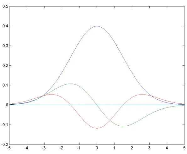
2.4 Gaussian (Blue), 1st and 2nd derivative of Gaussian (Green, Red) . . . 27

2.5 Find the best match of 2ndderivative of gaussian ∂ 2_G ∂x2 for box function . . . 29

2.6 Convolution of 1D Box Function With 2nd_{Derivative of Gaussian . . . 30}

2.7 2D Vessels . . . 32

2.8 Eigenvalues of The Hessian Matrix for 2D Vessels . . . 34

2.9 2D Balls . . . 35

2.10 First and Second Derivative of Gaussian in 2D . . . 36

2.11 Eigenvalues of The Hessian Matrix for 2D Balls . . . 37

2.14 Vesselness With Different Sigmas . . . 45

2.15 Comparing Original Data and Vesselness . . . 46

2.16 Comparing Original Data and Vesselness (Cross Sections) . . . 47

3.1 Different Situations When Comparing Neighbours With Non-maximum Sup-pression in 3D . . . 51

3.2 Pairwise Interaction Approximating Curvature [34] . . . 53

3.3 Vessel Thinning . . . 57

3.4 Line Interval Fitting . . . 58

3.5 Ball Fitting . . . 59

4.1 Minimum Spanning Tree on Connected Graph . . . 61

4.2 Original Graph . . . 61

4.3 Prim’s Algorithm . . . 62

4.4 Kruskal’s Algorithm . . . 62

4.5 Minimum Spanning Tree on Discrete 2D Points . . . 64

4.6 Minimum Spanning Tree on 2D Lines . . . 64

4.7 Minimum Spanning Tree on Data Thinning . . . 65

4.8 Minimum Spanning Tree on Line Intervals . . . 65

5.1 Pipeline of The Algorithms . . . 67

A.1 Maximum Intensity Projection . . . 73

A.2 Comparing Between Normal Projection and Maximum Intensity Projection . . 74

A.3 Cross Section of a Box . . . 75

A.4 Cross Section of The Vessel Volume . . . 76

B.1 Rings Reduction in Polar Coordinates [40] . . . 78

B.2 Comparison Before and After Rings Reduction . . . 79

D.1 Distance From Point to Line in 3D . . . 82

D.2 Distance Between Lines in 3D . . . 83

2.1 Corresponding Shapes for Vessels in 3D, 2D and 1D . . . 24

3.1 Non-maximum Suppression in 3D . . . 50

Appendix A Visualization of 3D Data . . . 73

Appendix B Rings Reduction . . . 77

Appendix C Eigenvalues of a Symmetric Matrix . . . 80

Appendix D Distance in 3D Space . . . 82

Introduction

1.1

Problem Overview

This thesis focuses on extracting the topological structure of a 3D cardiac images. It consists

of three main parts: (a) image filtering to remove noise; (b) extracting the centreline of vessels;

(c) enforcing a tree structure for the vessel withminimum spanning tree.

Extracting vessel structure remains a challenging problem because of a number of

tech-nical problems. Due to partial volume, the intensity of small vessels become weaker or even

completely disappear. Acquisition artifacts, such as rings or random noise, are very common

in the data. Special image filtering is required to remove these artifacts from the data while

preserving the details of small vessels. Even after these filtering, it is still not easy to extract

the image structures which can be either the segmentation or the centreline of the object. Topo-logical constraints are enforced on the image structures in order to remove ambiguities in the

result. These technical problems are further discussed in Section 1.1.2.

Standard methods have problems in extracting vessel structures with topological constraints. Graph cuts [6] is a recent optimization-based algorithm for image segmentation. But its

over-smoothing problem tend to smooth out the thin structures. Different attempts are made to address this over-smoothing problem (see Section 1.2.3). An alternative approach for

extract-ing vessel structure is by extractextract-ing the centreline. This can be achieved by calculatextract-ing the

minimum path between two user input points. This will be further discussed in Section 1.2.4.

It is not easy to validate the algorithms for extracting vessel structures. Therefore different visualization methods are developed so that we are able to see the 3D volume better. Two

visualization methods are frequently used in this thesis: (1)maximum intensity projection; and (2) visualizing a arbitrary cross section of the volume. Please refer to Appendix A for more

details.

1.1.1

Input and Ideal Result

Our 3D CT data is provided by Roberts Research1. It is a volume of the mouse’s heart. The

actual physical size of the data is very tiny, while the resolution of the data is very high (585×

525×892).

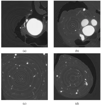
Figure 1.1 and Figure 1.2 show the original data. The bright parts correspond to vessels

and the dark parts to heart muscles and other injected material. Figure 1.1 shows four different slices of the original data. The bright white balls are corresponding to the cross sections of

arteries and the small white balls are cross sections for vessels. Figure 1.2 show the whole data

usingmaximum intensity projection. Some of the features of this data are:

1. The size of the vessels varies from tiny capillaries to arteries

2. Small vessels have lower intensity while thicker ones have stronger intensity

3. The partial volume problem exists at smaller vessels as well as on the boundaries of

bigger vessels

4. There are a number of artifacts of rings due to the reconstruction of the CT images

5. Random noise exists everywhere in the image

Figure 1.3b shows an example of the ideal result of this vessels.

(a) (b)

(c) (d)

Figure 1.2: Original Data With Maximum Intensity Projection

(a) Original Data (b) Ideal Result

1.1.2

Technical Problems

We are confronted with the three technical problems in order to get the result like those in

Figure 1.3b: (A) filtering (preprocessing),(B) structure extraction,(C) topological constraints. Filtering (preprocessing) reduces different kinds of noise in the image. Structures can be ei-ther the segmentation or the centreline of the object. In this thesis, we are focused on extracting

the centreline of the vessels. We conjecture that it is straight forward to get the segmentation

given a correct centreline. Finally, topological constraints are enforced on the centrelines using

minimum spanning treealgorithm.

(A) Filtering (Preprocessing)

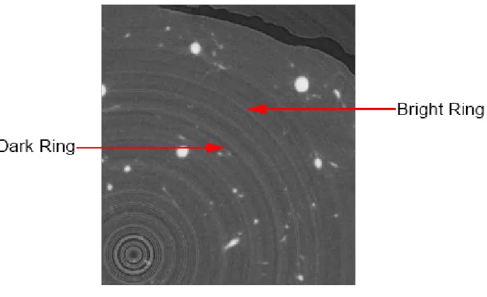
There are two kinds of noise in our data — rings and random noise. Rings illustrated in Figure 1.4 are very common in CT images. They are concentric rings superimposed on the image

while it is being scanned [24]. Rings are a structure noise in the following sense. For all points

that are with the same distance to the centre of rings, the variation of intensity is similar. Figure

1.4 shows a dark ring and a bright ring in the image. Random noise is variation of intensity

caused by the limitation of the digital sensors. Both of these noises are problematic; therefore

image filters are required in order to remove the artifacts.

Ring Filter

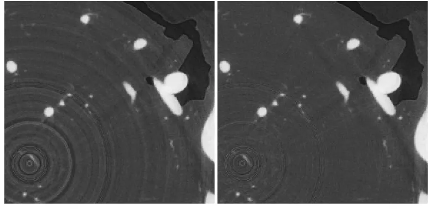
The state-of-the-art ring filter was proposed by [40] using mean and median filtering. Rings

artifacts are reduced to a great extent with this filter. Data before and after rings reduction are

shown in Figure 1.5. More details about this filter is presented in Appendix B.

Vesselness Filter

Standard filters such asGaussian filter,mean filter, ormedian filterare commonly used for non-structured white noise. They do not work well for our data because they smooth out the

small vessels. We apply the vesselness filter [29] to our data. This filter can remove background

noise while preserving structure details for small vessels. Figure 1.6 shows an image before

and after vesselness filter. Section 2 is focused on vesselness filter. We sometime refer to it as

“vesselness measure” and we use both of these two expressions in this thesis.

(B) Structure Extraction

There are two categories of methods to extract the structure of the object. Methods such as

graph cutssegment the object of interest by labelling all image pixels into two subsets: object or background [6, 43, 25]. Some skeleton-based methods extract the centreline of the object

[11, 14, 15, 28, 14]. Both extracting segmentation and extracting centreline are ill-posed

Figure 1.4: Rings Artifacts

Segmentation

Image segmentation is the process of assigning different labels to image pixels according to their image attributes such as intensity, colour and etc. Binary segmentation labels the image

into two subsets — foreground or background. One simple methods for image segmentation is

thresholding. It segments an image as follows: if the intensity of a point is above the threshold,

it is assigned to one label; otherwise it is assigned to the other label. Figure 1.7 shows an

example of binary segmentation using thresholding. Rings as well as other image noise are picked up with a low threshold. The result is cleaner with a high threshold, but some of the

small structures are lost. That is why thresholding does not work for our data and we need to

use more advanced and sophisticated methods.

Centreline

Another way to analyze our data is to extract the centreline of vessels. The concept of

centreline was first introduced by Blum et al [4]. It was originally referred to as thetopological skeletonin [4]. It is nowadays also known asmedialorsymmetric axes[44]. A centreline is a continuous imaginary line through the centre of an object. Every point on the centreline must

have more than one closest point to the boundary of the object.

The actual representation of the centreline is sometime referred to as discrete centreline

[44]. It can be represented in different ways. For example, it can be described as a set of independent points [44, 37, 28] (see Figure 1.8a). Centreline can also be represented as a set of

line intervals (see Figure 1.8b). We define thediscrete centrelineas follows: a connected graph with certain properties for nodes (as being either pixels or line intervals) that are equidistant

(a) Before Rings Reduction (b) After Rings Reduction

Figure 1.5: Rings Reduction

(a) Before Vesselness Filter (b) After Vesselness Filter

Figure 1.6: Vesselness Filter

(a) Original Data (b) Low Threshold (c) High Threshold

tree(see more in Section (C) bellow). Figure 1.10b and Figure 1.11b shows some examples of discrete centrelines on real data.

For simplicity, we refer both continuous centrelineanddiscrete centrelineas centreline in the rest of this thesis.

(a) With Points (b) With Line Intervals

Figure 1.8: Discrete Centrelines

(C) Topological Constraints

To disambiguate our ill-posed structure extraction problems discussed in (B), different topo-logical constraints can be enforced on the extracted structures. Two of the most important

constraints areconnectivity constraintandtree-connectivity constraint. Connectivity Constraint

The connectivity constraint for segmentation ensure the following — there exists a path

between any two points labelled as the same segment. Figure 1.9 shows an example of a

segmentation without connectivity constraint. Notice that the fins of the birds are separated from the body.

A graph that satisfy a connectivity constraint can have loop. Figure 1.10c shows an

ex-ample of enforcing connectivity constraint on the data points. The data points are pixels that

are correlated to the centreline of the vessel. The green lines in Figure 1.10 are the

connec-tion between data points. Notice that we may have loops in the result with only connectivity

constraint.

Tree-connectivity Constraint

A tree-connectivity constraint requires that the connective graph cannot have loops. Figure 1.10d show an example of enforcing the tree-connectivity constraint on the data points. Figure

1.11c shows an example of enforcing connectivity constraint on line intervals (red). The green

lines indicate the connectivities.

Figure 1.9: Segmentation Without Connectivity [43]

(a) Original Data (b) Data Points

(c) Connectivity (d) Tree-Connectivity

Figure 1.10: Centre Line With Data Points

1.1.3

Pipeline of The Algorithms

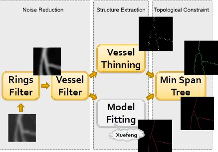
Figure 1.12 shows the pipeline of the algorithms. Our final goal is to extract the tree structures

of the cardiac image. The tree constraint is enforced with a minimum spanning tree algorithm.

Before building a tree, we have to construct a connected graph. Vessel thinning and model

(a) Original Data (b) Line Intervals (c) Tree Connectivity

Figure 1.11: Centre Line With Line Intervals

fits line intervals to the vessels.

The first block of the pipeline is noise reduction. Two different filters are applied to the original data in order to remove moth rings artifacts and random noise.

1.2

Related Work

Thin structures are very common in medical image processing, and a lot of research has been

done during the past decades. The research deals with at least one of the technical problems

that we discussed in Section 1.1.2. The organization of this section is as the following.

Section 1.2.1 and Section 1.2.2 summarize related works about two different filters used in this thesis: rings filterandvesselness filter, which are related to Technical Problem (A).

Section 1.2.3 introducesgraph cuts[6] which is focused on the segmentation of the object. Section 1.2.4 introduces some other methods, which are used to extract the centreline of the

object. Topological constraints are enforced on both of these two types of methods. Section

1.2.3 and Section 1.2.4 are related to Technical Problems (B) and (C).

1.2.1

Rings Filtering

Rings artifacts are a number of concentric rings superimposed on the image while it is being scanned [24]. The presents of rings causes problem for post processing, such as noise reduction

or image segmentation. Removing or reducing such artifacts is necessary and a lot of research

has been done on that over the past decade.

Rings reduction can be done while the CT image is being scanned. They are referred to

as processing algorithms for rings reduction. Algorithms such as [1, 45, 32] are all

[40, 2, 35, 27]. They are usually referred to as post-processing algorithms. In this thesis, we

are only focused on the post-processing algorithms.

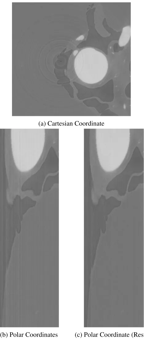
The state-of-the-art rings post-processing algorithm for rings reduction was initially

pro-posed by Sijbers and Postnov [40]. The algorithm transforms the image from Cartesian coor-dinate to polar coorcoor-dinate. Figure 1.13a shows an image with rings and Figure 1.13b shows its

corresponding polar coordinate image. The problem of the ring artifacts in the original image

becomes a problem of line artifacts in the polar coordinate image. And then a mean filter is

applied to the image in polar coordinate. A artifacts template is generated by comparing the

image before and after mean filter. The rings are corrected based on the artifacts template.

Figure 1.13c shows the result after reducing the line artifacts in polar coordinate. Finally the

image is transformed back into Cartesian coordinates.

Many algorithms are based on the method described above such as Axelsson et al. [2].

However, the filtering does not necessary have to be done under polar coordinates. A similar algorithm in Cartesian coordinate is introduce by Prell et al. [35]. Some comparison of the

ring filter under Cartesian coordinate and polar coordinates can be found in Prell et al. [35] and

Kyriakou et al. [27].

1.2.2

Vesselness Filtering

The vesselness filter was introduced by Frangi et al. [19]. It was initially called vessel en-hancement filter in [19] because of the fact that this filter can reduce unexpected white noise in the image while preserving vessel structures. It is later referred to as vesselness measure

[9, 10, 17] or vesselness filter [36, 18, 41]. In this thesis, we use both of the terminologies interchangeably.

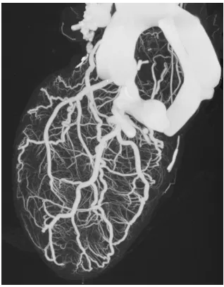
The vesselness measure proposed by [19] calculate the measure indicating how likely a

point belongs to a vessel. A critical steps is computing the Hessian matrix from the image data.

This filter can also detect the major orientation of the vessels by computing the eigenvalue

decomposition of the Hessian matrix. Figure 1.14 shows an example of vesselness measure

computed from [19]. More details on this method are introduced in Chapter 2.

The vesselness filter is later used in many other applications. For example, it is used for

(a) Cartesian Coordinate

(b) Polar Coordinates (c) Polar Coordinate (Result)

(a) Original Image (b) Vesselness Measure

1.2.3

Graph Cut Segmentation

Graph cut has been widely use because of its capability in dealing with graph-based energy

[6, 5]. It formulates the graph energy into the following:

E(f)= X p,q∈N

Vp,q(fp, fq)+

X

p∈P

Dp(fp), (1.1)

whereVp,q(fp, fq) is the smooth cost for any neighbouring pixelspandqunder a neighbourhood systemN; andDp(fp) is data cost for any pixel in the set of image pixelsP.

This smooth cost in graph cuts is for handling image noise. However, it has the an

over-smoothing problem for thin structures. We refer to this as the over-over-smoothing problem. As is

illustrated in Figure 1.15, the feet and the tentacles of the bee are lost with graph cuts

segmen-tation method.

(a) Original Image (b) Ground Truth (c) Graph Cut

Figure 1.15: Over-smoothing of Thin Structure With Graph Cuts [25]

Multiple attempts have been made by previous researchers in order to address the

over-smoothing problem. An attempt is through coupling edges in graph cuts [23, 26]. They achieve

this by categorizing the image edges into groups and applying some discount function on graph

cuts if some edges in the same group are cut. Take the image of the bee (Figure 1.15) as an

example. The tentacles of the bee are thin structures. Therefore, the smooth cost is very high in

order to segment the tentacles. But the boundary edges of the tentacles have similar appearance

— dark on one side and bright on the other side. The edges along the boundary of the tentacles can be categorized as the same group. The smooth cost for these edges of the same group are

reduced in order to segment thin structures such as the tentacles. The problem of this approach

is that the categorization of the edges is not reliable. Therefore, some other image noise or

artifacts are introduced to the final segmentation.

cuts. A interactive method is proposed by Vicente et al. [43]. This method first get an initial

segmentation using graph cuts (Figure 1.16a). Then user can add additional input points and

these points will be connected to the initial segmentation usingDijkstraGC algorithm. Please refer to Vicente et al. [43] for more details about theDijkstraGC algorithm.

(a) Initial Segmentation (b) Additional User Input (c) Final Segmentation

Figure 1.16: Connectivity Constraint in Graph Cut [43]

1.2.4

Centreline-Based Methods

The centreline of tubular structures are extracted by computing the minimal path between two

user-input points [11, 14, 15]. It can detect global minimum of an active contour model’s

energy between two endpoints [11].

The benefits of the minimal path approach include global minimizers, fast computation and

incorporation of user input. A drawback of this approach is that it represents the vessel with a

curve which runs through the interior of the vessels instead of a full tubular surface. In order

to overcome this, a fourth dimension of the vessel is introduced by [28], which is the radius

of the vessel. Each point on the 4-D curve consists of 3 dimensional spatial coordinates plus

a fourth dimension which describes the radius of the vessel at that corresponding 3-D point in

space [28]. Thus, each 4-D point represents a sphere in 3-D space, and the vessel is obtained

by taking the envelope of these spheres as we move along the 4-D curve. This approach takes

into consideration both the mean and variances for sphere sp = (p,r) in an image where p

is 3D points andr is radius. Finally they compute the minimum path between two user input spheres. Please refer to Li and Yezzi [28] for more details.

Some of the results of the 4D path approach are shown in Figure 1.17. Notice that the

connectivity constraint is automatically enforced when computing the minimum path between

two user input points.

These centreline-based methods are normally applied for extracting centrelines of colons

because a colon has only two endpoints. It is not applicable to vessels because the number of

Figure 1.17: 4D Path Result [28]

1.3

Contributions

We gave a more intuitive explanation of the vesselness filter in Chapter 2. We explained in

detail why this measure works for 3D tabular structures. And also we discussed about different ways of adjusting this filter so that it can be used for detecting other image structures (such as

balls on 2D images).

We implemented and compared two different methods for extracting the centrelines of the vessels in Chapter 3. We developed avessel thinningmethod inspired bynon-maximum sup-pression. Our colleague Xuefeng Chang implemented the recent optimization-based model fitting algorithm. We shows an simpler model fitting problem in Section 3.3.2.

In Chapter 4, we implemented aminimum spanning treealgorithm and used it to enforced the tree-connectivity constraint on both of the two types of centrelines.

Finally, we implemented visualization tools in order to better analyze our data. We are able

to visualize themaximum intensity projectionand an arbitrary cross section of the 3D data.

1.4

Outline of the Thesis

Vesselness filter (or vesselness measure) is explained in detail in Chapter 2. The use of the

Harris conner detector is very similar to the use of vesselness filter and it is presented in Section 2.2. TheHessian matrixis used for the vesselness filter and it is explained in Section 2.3 and Section 2.4. In Section 2.5 and Section 2.6, the eigenvalues of Hessian matrix are described.

Two different methods of extracting centreline of the vessel are explored in Chapter 3. This thesis is focused on the first method — data thinning in Section 3.2. A second method is mostly carried out by a colleague, Xuefeng Chang. Some brief introduction of model fitting is

presented in Section 3.3.

The use ofminimum spanning treeis explained in Chapter 4. Two commonly used algo-rithms for computingminimum spanning treeis presented in Section 4.1. The use ofminimum spanning treealgorithm on our data is discussed in Section 4.2 and Section 4.3.

Notice that visualization is also a very important part of the project. Some of the

implemen-tations of visualization are explained in Appendix A. A rings filter is implemented according

to [40] and it is briefly introduced in Appendix B. Appendix C introduces some well-known

properties for eigenvelues and eigenvector that are used in Chapter 2. Appendix D introduce

Vesselness Measure

2.1

Overview

The vesselness measure intuitively describe the likelihood of a point being part of a vessel. The

higher the value of the vesselness of a given point, the more likely it is vessel. The vesselness

measure uses a combination of Gaussian filter and Hessian matrix, which was proposed in Frangi et al. [19]. This method first was introduced in 1998 and became a gold standard for

vesselness measure ever since then. Some related work has been introduced in Section 1.2.2.

The terminologies vesselness measure and vesselness filter are equivalent and we use them iteratively in this chapter.

It is not reliable to judge weather a point belongs to a vessel or not based the intensity of

that point. The vesselness measure takes advantage of the following two properties for a vessel:

(a) the intensity stays unchanged along the direction of a vessel; (b) the intensity varies a lot

in the normal direction of a vessel. Vesselness measure is capable of aggregating the intensity

information of neighbouring points using Gaussian filter. It can also be derived for the major orientation of the vessel by computing the eigenvalue decomposition of the Hessian matrix. As

a result, it is very powerful in suppressing background noise.

We start this chapter with a Harris corner detector in Section 2.2. The Harris corner de-tector is a well-known image corner dede-tector in Computer Vision. It is similar to vesselness

filter and it can be easily derived geometrically. Explaining the Harris corner detector will help

with the describing of vesselness filter. Harris corner detector and vesselness filter have the

following similarities:

1. Both of them extract the major orientation of local image structures based on eigenvalue

decomposition;

2. Both of them are using 3×3 matrices for 3D images (or 2×2 matrices for 2D images);

3. Both of them aggregate intensity information of neighbouring points.

We explain the vesselness filter in Section 2.3. Section 2.3 explains the vessels in 1D and

2D with respect to vessels in 3D. Hessian matrix is discussed in Section 2.4. We explain why

we have to combine the Gaussian filter with Hessian matrix. Section 2.5 describe different ways of combining of the eigenvalues and explain why the current vesselness detector is being

used. Section 2.6 explains how to decide the correct scale of the vessel.

2.2

Harris Corner Detector

The original idea of Harris corner detector was proposed by Harris and Stephens [20]. A very

good derivation is available in Derpanis [13].

2.2.1

Derivation of The Matrix for Harris Detector

The main goal of the Harris corner detector is detecting the shape corners in an image. It is

impossible to tell whether this point belongs to a corner or not based on the intensity of one

point. That’s why Harris corner detector makes judgement based on a set of points within a

certain windowsW. The sum (or weighted sum) of the intensities within a certain window is computer. If the shifting of a windowWin any direction would give a large change in intensity, then a corner exists at that position. The change of intensity for the shifts= [∆x∆y]T _is:

d(∆x,∆y)= X W

w(x,y)[I(x+ ∆x,y+ ∆y)−I(x,y)]2,

wherew(x,y) is a weight function. That is either a rectangular function ω = 1 or a Gaussian weighting functionω =e−(x2+y2)/(2σ2).

The shift image intensity is approximated by a Taylor expansion truncated to the first order

terms,

I(x+ ∆x,y+ ∆y) ≈ I(x,y)+Ix∆x+Iy∆y

= I(x,y)+sT · ∇I,

Therefore,

d(∆x,∆y) = P

W

w(x,y)[I(xi + ∆x,yi+ ∆y)−I(xi,yi)]2

≈ P

W

w(x,y)[sT∇I]2

= P

W

w(x,y)[sT∇I∇ITs]

= sT P

W

w(x,y)∇I∇IT

!

s

(2.1)

Let M(x,y) be a 2×2 matrix computed from image derivatives,

M(x,y)= X W

w(x,y)· ∇I· ∇IT =X

W

w(x,y)

      

I2x IxIy

IyIx Iy2.

       (2.2)

Then Equation (2.1) can be further written as,

d(∆x,∆y)= sTM(x,y)s. (2.3)

2.2.2

Eigenvalues and Eigenvectors of Harris Detector

Letλi theitheigenvalue of matrix M(x,y) andvi be the corresponding eigenvectors. Based on the definition of eigenvalues and eigenvectors, we have,

M(x,y)vi = λivi. We can left multiplyvT

i on both sides giving:

vTi M(x,y)vi = λivTi vi, (2.4) Ifviis a unit vector (vT_ivi = 1), then Equation (2.4) can be written as,

vTi M(x,y)vi =λi. (2.5) Comparing Equation (2.5) and Equation (2.3), it is not hard to see the geometric meaning

of eigenvalues —– the eigenvalueλi describe the variation of image intensity along direction

vi.

It can be proofed thatλiis real number rather than complex (Theorem C.0.1) and the eigen-vectors are always perpendicular to each other (Appendix Theorem C.0.2).

Because of the fact that the eigenvalues of M(x,y) are independent to the choice of s =

the current position (x,y). And these properties are,

• λ1 ≈0,λ2 ≈0

If bothλ1,λ2 are small, the windowed image region is of approximately constant inten-sity.

• λ₁ ≈0,λ2 0

If one eigenvalue is high and the other low, only local shifts in one direction (along the

ridge) cause little change in d(x,y) and significant change in the orthogonal direction. This indicates an edge.

• λ₁ 0,λ2 0

If both eigenvalues are high, then shift in any direction results in a significant increase.

This indicates a corner.

2.2.3

Visualization of Eigenvalues and Eigenvectors

M(x,y) can be represented via the following ellipsoid:

sTM(x,y)s=1. (2.6)

Eigenvalue decomposition gives:

M(x,y)=UΛUT,

whereΛis a diagonal matrix and U is a rotation matrix:

Λ =       

λ1 0 0 λ2

     

 and U =        v1

v2.

      

Applying this to Equation (2.6) we have,

sTUΛUTs= (UTs)TΛ(UTs)=1

By rotating the coordinates fromstos0_throughs0= _UT_s=_[∆_x0,∆_y0_]T_{, we gets}0TΛ_s0 = _1. That is,

λ1∆x 02_+λ

2∆y

02₌ ∆x 02

1

√

λ1

!2 +

∆y02

1

√

λ2

Figure 2.1: Visualized Eigenvalues with Ellipsoid

The semi-principal axes of the ellipsoid are √1

λ1

, and √1

λ2

. It can visualized as Figure 2.1.

2.2.4

Combination of Eigenvalues

A proper combination the eigenvalues is needed in order to get a descriptive corner measure.

The Harris corner detector looks for the feature with bothλ1 0 andλ2 0. There are many options including but limited to the following.

1. In the original paper, Harris and Stephen [20] use the following measure (with the value

ofκto be determined empirically),

R = λ₁λ₂−κ·(λ1+λ2)2

= det(M)−κ·trace2(M).

2. Shi and Tomasi [39] compute the minimum of the eigenvalues as the corner feature

response,

R= min(λ1, λ2).

3. Noble’s [33] corner measure computes the harmonic mean of the eigenvalues

2.3

Conceptual Vessels in Di

ff

erent Dimensions

It is easier to describe the vesselness filter is 1D and 2D and then upgrade it to a higher

dimen-sion. Therefore, we describe the corresponding shapes in 2D and 1D images for a 3D vessels.

We will discuss why the downgrading is reasonable and what information is preserved or lost

during the downgrading.

The degree of freedom of shapes in different dimensions are summarized in Table 2.1. Dimension Shape Representation Degree of Freedom

3D Tube 7

2D Rectangle 5

2D Ball 3

1D Box Function 2

Table 2.1: Corresponding Shapes for Vessels in 3D, 2D and 1D

2.3.1

3D Vessels as Tubes

In 3D, vessel can be thought of as a set of 3D tubes. Each tube have two end points (6 degrees

of freedom) and one radius (1 degree of freedom); therefore there are 7 degrees of freedom in

total.

2.3.2

2D Vessels as Rectangles and Balls

There are two different ways to project a 3D vessel onto a 2D plane.

If the projection plane is parallel to the orientation of the vessel, the vessels are projected

as rectangles (Figure 2.2a). There are 5 degrees of freedom for a rectangle — two endpoints (4

degrees of freedom) and a radius (1 degree of freedom).

If the projection plane is perpendicular to the orientation of the vessel, the projection of the

vessels become balls (Figure 2.2b). There are only 3 degrees of freedom for a ball — two for position and one for radius.

Degrading the 3D tubes to 2D rectangles can preserve the orientation information of

ves-sels. However, the orientation can be handled with Hessian matrix easily (as is shown later in

Section 2.4). It is the distance to the centreline of the tubes that matters. Therefore, it is also

reasonable to degrade the 3D tubes to 2D balls. We will describe Hessian matrix for both cases

(a) Rectangle, 5 Degree of Freedom (b)

Figure 2.2: Conceptual Vessels in 2D

2.3.3

1D Vessels as Box Functions

The projection of 2D vessel (rectangle) along the orientation of the vessel is a 1D box function

as the following,

f(x)=

      

C if|x−µ|<r

0 otherwise (2.8)

whereCis a constant,µis the center of the box function andris the size (or radius) of the box function. A 1D box function has 2 degrees of freedom.

2.4

Hessian Matrix and Gaussian Derivatives

Hessian matrix and 2nd _{derivative of Gaussian filter are the two most important concepts used}

for vesselness filer. We first explain the use of the 2nd derivative of Gaussian to detect the

box functions in a 1D image (Section 2.4.1). And then the Hessian matrix is combined with

Gaussian in order to detect 2D balls and rectangles in the images (Section 2.4.3 and Section

2.4.2). The detection of 3D tubes (or vessels in 3D) are introduced in Section 2.4.4.

2.4.1

Second Derivative of Gaussian in 1D

Assume that we have a 1D image, which can be described as a 1D discrete function. This 1D

image contains some box functions with unknown centres and radii (Figure 2.3). The goal is

We use the second derivative of the Gaussian function to achieve this. The equations for

Gaussian, first derivative of Gaussian, and second derivative of Gaussian are shown as follows.

• Gaussian

G(x)= √1

2πσe −(x−µ)

2

2σ2

• Derivative of Gaussian

∂G(x)

∂x = − x−µ √

2πσ3e −(x−µ)

2

2σ2

• Second derivative of Gaussian

∂2_G(x) ∂x2 =

(x−µ)2−σ2

√

2πσ5 e −(x−µ)

2

2σ2 _(2.9)

The equations are plotted in Figure 2.4.

Figure 2.4: Gaussian (Blue), 1st_{and 2}nd_{derivative of Gaussian (Green, Red)}

For the second derivative of Gaussian Equation (2.9), notice that it is smaller than zero

within [−σ+µ, σ+µ], and greater than zero elsewhere.

Assume that µand σof the 2nd _{derivative of Gaussian matches the centre and radius of a}

Z σ+µ

−σ+µ

∂2_G(x)

∂x2 f(x)dx = C · ∂G(x)

∂x σ+µ −σ+µ

= −C√(x−µ)

2πσ3 e −(x−µ)

2

2σ2

σ+µ −σ+µ

= −C(σ√+µ−µ)

2πσ3 e

−(σ+µ−µ)

2

2σ2 + C(−σ_√+µ−µ)

2πσ3 e

−(−σ+µ−µ)

2

2σ2

= −√2Cσ

2πσ3e −1 2 = − r 2 eπ C

σ2.

(2.10)

Notice that if we have a positive box function with f(x)=Cgreater than 0 within the box, the result of the convolution is a negative value. We refer to the absolute value of the result of

convolution as the response.

If and only if µandσ of the 2nd derivative of Gaussian matches the centre and radius of

a box function, the convolution generate a highest response. This argument is illustrated by Figure 2.5. In the Figure 2.5, the red lines represent the box function and curves represent

a second order of derivative of Gaussian. We draw the negative of the second derivative of

Gaussian for better visualization. In Figure 2.5a, all three second derivative of Gaussian have

the same mean value µ. Sigma of the blue Gaussian is the same with the radius of the box

function, while sigma of the purple and green one are smaller and bigger respectively. In

Figure 2.5b, all three second derivative of Gaussian have the same varianceσ. The blue one is

consistent with the box function. The other two are sifted to the right and the left a little bit.

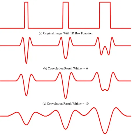
For example, the three boxes in Figure 2.3 are with the radii of 6 pixels, 10 pixels and 20

pixels respectively. We compute the convolution with the second derivative of Gaussian with the images for all image position µand three different sigmasσ = 6, σ = 10 and σ = 20, which matches the radii of the box functions respectively. The responses are displayed in

Figure 2.6a-c. Notice that whenever the sigma of 2nd_{derivate of Gaussian matches the radii of}

(a) ∂

2_G

∂x2 with different sizes

(b) ∂

2_G

∂x2 with different centres

Figure 2.5: Find the best match of 2nd_{derivative of gaussian} ∂ 2_G

(a) Original Image With 1D Box Function

(b) Convolution Result Withσ=6

(c) Convolution Result Withσ=10

(d) Convolution Result Withσ=20

2.4.2

Hessian for Rectangles in 2D

We need to consider the orientations of vessels in 2D images, which can also be considered as

rectangles (see Section 2.3.2). One very intuitive way to deal with this problem is to use filters

with different orientations. However, filters with multiple orientations are hard to design and the running speed can be slow.

In Section 2.2, the use of Harris corner detector is invariant to orientation. Is there a filter that can measure the vessel and is invariant to vessel orientation? We can achieve this with

Hessian matrix.

The Hessian matrix in 2D is given by,

H(f)=

                   

∂2_f ∂x2₁

∂2_f ∂x1∂x2 ∂2_f

∂x2∂x1

∂2_f ∂x2₂

                    ,

where f is 2D discrete function. Each entry of the Hessian matrix is a second derivative of function f.

In order to use the Hessian matrix for vessel detection, we need to use it along with a

Gaussian filter G. We first blur our image I with the Gaussian filter and then compute the Hessian matrix on the blurred imageH(G ∗ I). The benefit of doing this is illustrated in rest of this section.

Figure 2.7 shows an example of 2D vessel as 3 bright rectangles. All these three rectangles

are aligned with the y axis, which indicates that the image does not have a gradient along the y

direction; Therefore, the following entries in the Hessian matrix are zero

H₁₂(f) = ∂ 2_f

∂x∂y = 0

H₂₁(f) = ∂ 2_f

∂y∂x = 0

H₂₂(f) = ∂ 2_f

Figure 2.7: 2D Vessels

And the value ofH11is

H₁₁(f) = H₁₁(G ∗ L)

= _∂∂

x ∗

∂

∂x ∗ G ∗ I=0

= ∂_∂2G

x2 ∗ I

H₁₁is the convolution of the second derivative of Gaussian Equation (2.9) with our image, which is used for the 1D box function in Section 2.4.1. Based the previous discussion, if the

sigma of the Gaussian matches the size of the vessel, the highest response is generated at the

centre of the vessel.

The radii for the vessels in Figure 2.7 are 6 pixels, 10 pixels, and 20 pixels respectively.

Figure 2.8a show the centre row thatH₁₁ is computed with green dash lines. The sigmas of Gaussian filters that used for Figure 2.8b-d are 6 pixels, 10 pixels, and 20 pixels respectively.

Notice that we always have the best response when the sigma of the Gaussian filter matches

the vessel size.

If the orientation of the vessel is aligned with the xaxis, the image gradient along the x axis is zero. The only non-zero entry in the Hessian matrix isH₂₂. Similarly, the best response of the convolution is

H₂₂ = ∂

2_G ∂y2 ∗ I

How about a vessel with an arbitrary orientation? We can address this by computing the

eigenvalues and eigenvectors for the Hessian matrix. Let λ1 and λ2 be the eigenvalues of the

Hessian matrixH, and the corresponding eigenvalues bev1andv2. The Hessian matrix can be decomposed into the following form using eigenvalue decomposition.

whereΛis a diagonal matrix and U is a rotation matrix, Λ=       

λ1 0 0 λ2

     

 and U=        v1 v2        .

This implies that we can rotate the image using a rotation matrix U so they align with the axis. The geometric meaning of the eigenvalueλiis the convolution of the image with a second

order derivative of Gaussian on the direction ofvi.

Intuitively, if a pixel is close to the centreline of a vessel, it should satisfy the following two

properties:

1. one of the eigenvaluesλ1should be very close to zero;

2. the absolute value of the other eigenvalue should be a lot greater than zeroλ2>>0.

Therefore, if we sort the eigenvalues based on their absolute values so that

|λ₁|<|λ₂|,

we can use the absolute value of second eigenvalue|λ₂|as a intuitive measure about how close a pixel is to the centre of the vessel.

(a) Original Image

(b)σ=6

(c)σ=10

(d)σ=20

2.4.3

Hessian for Balls in 2D

The cross section of 3D vessels are 2D balls. Figure 2.9 gives us an example.

Figure 2.9: 2D Balls

In the Section 2.4.2, the intensity of the image stays constant along the orientation of the

vessel. Blurring the image with Gaussian filter along the orientation of the vessel won’t have

any effects.

For balls, we need to look into the properties of the 2D Gaussian functions. The relationship between the Gaussian in 2D and 1D is shown in the following equations. Figure 2.10a shows

an example of the first derivative of 2D Gaussian. Figure 2.10b shows an example of the second

derivative of 2D Gaussian.

• Gaussian

G(x,y)=G(x)· G(y)

• Derivative of 2D Gaussian

∂G(x,y)

∂x =

∂G(x)

∂x · G(y)

∂G(x,y)

∂y =

∂G(y)

∂y · G(x)

• Second derivative of 2D Gaussian

∂2_G(x,_y)

∂x2 =

∂2_G(x) ∂x2 · G(y) ∂2_G(x,_y)

∂y2 =

∂2_G(y) ∂y2 · G(x) ∂2_G(x,_y)

∂x∂y =

∂G(x)

∂x ·

∂G(y)

∂y

(a) ∂G_∂(x,y)

x (b)

∂2_G(x,y)

∂x2

Figure 2.10: First and Second Derivative of Gaussian in 2D

our coordinate system. The equations for the Gaussian filter and the ball is show as:

G(x,y)= 1 2πσ2e

−x

2_+y2

2σ2 , _(2.11)

F(x,y)=

      

C if x2+y2< r2

0 otherwise . (2.12)

Now the Gaussian only have one parameter — the varianceσ. And Ball function also has

only one parameter — the radius of the ballr. The convolution of the Equation (2.11) and Equation (2.12) gives,

R(σ,r) =

" _∂2

G(x,y)

∂x2 · F(x,y)dxdy

= −C · r

2

2σ4e − r

2

2σ2_.

(2.13)

The result of the convolution is related to both the radius of the ball (r) and the variance of the Gaussian function (σ). We can get the extreme function value by taking the partial

derivative ofR(σ,r) overr:

∂R(σ,r)

∂r = (

r2

2σ2 −1)·

r

σ4 ·e − r

2

(a) Original Image

(b) Eigenvalues

Figure 2.11: Eigenvalues of The Hessian Matrix for 2D Balls

Whenr= √2σ, the partial derivative above equals to zero andR(σ,r) reaches minimum

R(σ,

√

2σ)= − 1

σ2_e. (2.15)

We compute the eigenvalues of the Hessian matrix for Figure 2.9. We plot the eigenvalues

along the centre row of the image as illustrated by Figure 2.11a. The sigma of the Gaussian

is √10

2, which matches the radius of the second ball. As a result, Figure 2.11b shows that the highest response at the centre of the second ball.

Now we need to combine these two eigenvalues as one measure. The following are all

reasonable options:

• −(λ1+λ2), Figure 2.12(a)

• λ₁λ₂, Figure 2.12(b)

• λ2₁+λ2₂, Figure 2.12(c)

• max(|λ₁|,|λ₂|), Figure 2.12(d)

• −min(λ1, λ2), Figure 2.12(e)

(a)−(λ1+λ2)

(b)λ1λ2

(c)λ2₁+λ2₂

(d)max(|λ1|,|λ2|)

(e)−min(λ1, λ2)

2.4.4

Hessian for Vessels in 3D

Hessian matrix in 3D is given by the following equation,

H(f)=

                             

∂2_f ∂x2₁

∂2_f ∂x1∂x2

∂2_f ∂x1∂x3 ∂2_f

∂x2∂x1

∂2_f ∂x2 2

∂2_f ∂x2∂x3 ∂2_f

∂x3∂x1

∂2_f ∂x3∂x2

∂2_f ∂x2₃

                              .

There are three eigenvaluesλ1,λ2andλ3with the corresponding eigenvectorsv1,v2andv3. We sort the eigenvalues so that,

|λ₁| ≤ |λ₂| ≤ |λ₃|

The Hessian matrix for 3D vessels is very similar to Hessian for 2D balls. For the three

eigenvalues of the Hessian in 3D, one of them should be very close to zero because the intensity of the image stays constant along the orientation of the vessel.

|λ₁| ≈0

The cross section of the 3D vessels are balls. The other two eigenvalues are equivalent to

the eigenvalues of the 2D Hessian calculated from the cross section of the vessel. Therefore, at the centre of the vessel, the two eigenvalues should be approximately equal to each other and

their absolute value should be much greater than zero.

|λ₂| ≈ |λ₃| 0

2.4.5

Hessian Matrix in General

In mathematics, the Hessian matrix is a square matrix of second-order partial derivatives of a

H(f)=                                          

∂2_f ∂x2 1

∂2_f ∂x1∂x2

· · · ∂

2_f ∂x1∂xn ∂2_f

∂x2∂x1

∂2_f

∂x2₂ · · ·

∂2_f ∂x2∂xn

... ... ... ...

∂2_f ∂xn∂x1

∂2_f ∂xn∂x2

· · · ∂

2_f ∂x2 n                                           . (2.16)

To analyze the local feature of an image, it is a common approach to consider the

neigh-bours of an imageI(x) at a point xusing Tyler expansion [19],

I(x+ ∆x)≈ I(x)+ ∆xTJ(x)+ ∆xTH(x)∆x (2.17) This approximates the image up to second order. J(x) is the Jacobian matrix of the image at position x, which is also equivalent to the gradient of the image 5I. ∆x is offset of the image position, and x+ ∆x give the position of the neighbouring location. AndH(x) is the Hessian matrix computed from the image at position x and it contains the information about the curvature of the image function.

ImageIis blurred from the original imageIo with a Gaussian filterG(σ)

I=G(σ)∗ Io

The Hessian matrix compute the second order derivative of the function. For each image

position, theith_{row and j}th_{column of the Hessian matrix is,}

Hi j(x)= ∂ ∂xi

∗ ∂

∂xj

∗ G(x, σ)∗ I(x)

where ∂

∂xi

is the derivative on theith_{dimension andG(x}, σ_{) is a Gaussian centred atx. Notice}

that both the derivative of the image ∂

∂xi

and the Gaussian filterG(x, σ) can be represented by convolution of matrices.

Let λk denote the eigenvalue corresponding to the kth normalized eigenvector uk of the Hessian matrixH(x). From the definition of eigenvalues,

Left multiply both sides of the equation gives,

uT_kH(x)uk = λk.

The benefits of eigenvalue analysis is to that it automatically extracts the principal

orienta-tion which gives the smallest and biggest semi-axis of the corresponding ellipsoid represented

by the matrix. The value of the k-th semi-axis is corresponding to √1

λk

. As for the Hessian

ma-trix, using the eigenvalue analysis, the local second order structure can be decomposed and this

directly gives the direction of smallest curvature [19]. The direction of the smallest curvature

is the orientation of the vessel.

2.5

Combination of Eigenvalues

Some examples of combination of eigenvalues were discussed in Section 2.4.3. A standard

combination of the eigenvalues for vesselness measure [19] is introduced in Section 2.5.1. We

also developed a alternation of the vesselness measure for ballness measure in Section 2.5.2.

2.5.1

3D Vesselness Measure

We sort the eigenvalues so that,

|λ₁| ≤ |λ₂| ≤ |λ₃|

If we are detecting bright vessels on dark background, both λ2and λ3 should be less than zero based on the previous discussion. If any of them are grater than zero, that voxel is most

likely a background voxel (vessel measure is set as zero). If both λ2 andλ3 are greater than

zero, the following three components are used for vesselness measure [19]:

• To differentiate between plate and line like structures,

A= |λ2| |λ₃|.

A → 0 implies a plane; A → 1 implies a line. This term can also be consider as the roundness of the vessel.

• To differentiate blob like structure,

B= √|λ1| |λ2λ3|

B → 1 implies that|λ₁| ≈ |λ₂| ≈ |λ₃|, which implies a blob like structure with equivalent curvature along all directions. Therefore, when building a vessel detector, we looking

for the opposite ofB.

• To differentiates between foreground (vessel) and background (noise),

S=

q

λ2 1+λ

2 2+λ

2 3

The smallerSis, the more likely the voxel belongs to background. Based on the previous discussion on eigenvalues on 2D balls (Figure 2.12c), it is obvious thatShas the highest value when close to the centreline of the vessel.

Finally, the formulation of the vessel measure by Frangi et al. [19] is as follows,

V=         

0 ifλ2 >0 orλ3> 0

(1−e−

A2 2α2_)e−

B2 2β2

(1−e−

S2 2γ2

) otherwise

(2.18)

The exponential function is used in order to map the measure to a value between 0 and 1.

α,βandγare parameters to tune.

2.5.2

2D Ballness Measure

A ball structure does not have any principle direction. Therefore, the two eigenvalues should be close to each other.

We also sort the eigenvalues so that

|λ₁| ≤ |λ₂|

Similarly, if we are detecting white balls on dark background, and if either λ1 or λ2 is

smaller than zero, the ball measure is set to zero. Otherwise, the following two components are

used for the ballness measure.

• To differentiate between plate and line like structures,

A= |λ1| |λ₂|

A →0 implies a line;A →1 implies ball.

• To differentiates between foreground (ball) and background (noise),

S=

q

λ2 1+λ

The smallerSis, the more likely the voxel belongs to background.

Finally, the ballness measure can be formulated as,

V=         

0 ifλ1> 0 orλ2 >0

(1−e−

A2

2α2_)(1−e−

S2 2γ2

) otherwise

(2.19)

The different terms of ballness are visualized in Figure 2.13. The sigma is equal to 5√2, which matches the size of the second ball. Therefore, the second ball has the highest ballness

response.

(a) Original Image

(b) 1−e− A2 2α2

(c) 1−e− S2 2γ2

(d) Ballness Result (1−e− A2

2α2_)·(1−e−

S2 2γ2

)

2.6

Comparison Between Scale

Scale is always an important factor for feature detector such as the SIFT feature [30]. If we

have two pictures of a same object taken from different distances, their sizes are different on the image. A good feature detector should still able to recognize them.

For vesselness measure, it is also very important to retrieve the size of the vessels. There are

multiple ways to achieve this [19, 31]. We adopted the method proposed by Frangi et al.[19]. The best response is selected among all scalesR(σ)=max

σi

R(σi).

From Equation (2.10), the best response of the convolution of the second derivative in 1D

with a box is,

R(σ) =

Z σ+µ

−σ+µ

∂2_G(x) ∂x2 f(x)dx

= − 1

σ2 ·

√

2C √

eπ

From Equation (2.15), we know the best response of the convolution of the second

deriva-tive in 2D with a ball is,

R(σ) =

" _∂2

G(x,y)

∂x2 · F(x,y)dxdy

= − 1

σ2 ·

C

e

Therefore, to make the the convolution result invariant to scale σ, we need to normalized our Gaussian filter with a scalerσ2_.

G0(σ)=σ2· G(σ) (2.20) However, not every term in the vessel measure in Equation (2.18) is affected by the scale problem. This following term is affected by the problem.

S=

q

λ2 1+λ

2 2+λ

2 3

These following two are irrelevant to scale because we are computing the ratio of the

eigen-values.

A= |λ2|

|λ₃|, B= |λ₁| √

2.7

Result

Figure 2.14 show the vesselness with different sigmas. Notice that with a small sigma, we can detect a lot of small vessels (Figure 2.14b). When we increase σ, we start to detect bigger

vessels however we lose the small ones (Figure 2.14c-d).

The vesselness is computed for all different scales and we choose the scale with the max-imum response. A comparison of the results of original image and the vesselness result are

shown in Figure 2.15 and Figure 2.16 with the visualization method discussed in Appendix

A.1. Figure 2.15b shows the result withmaximum intensity projection. Figure 2.15c shows the orientation of the vessels. Figure 2.16 show some arbitrary cross sections of the 3D volume

of the original data and vesselness filter. Notice that there is a grey background in the original

data, while the background noise is suppressed to a great extent in the vesselness measure.

(a) Original Data (b)σ=0.75

(c)σ=2.50 (d)σ=5.00

(a) Original Data

(b) Vesselness (c) Vessel Direction

(a) (b)

(c) (d)

(e) (f)

Centreline Extraction

3.1

Overview

The formal definition of centreline is given in Section 1.1.2. There are a couple of motivations

for extracting the centreline of the vessels:

1. in the context of information theory, we can make the data sparse so that we need less

number of bits to encrypt the data;

2. we can compute the topology of the vessels usingminimum spinning tree;

3. it is straight forward to reconstruct the segmentation of the vessel given the correct

cen-treline.

Some related methods about extracting centreline are resented in Section 1.2.4. We develop

two centreline approaches in this chapter: (1) Vessel Thinning; (2) Model Fitting.

Vessel Thinning

We get some intuition from Canny edge detector [8], which was developed by John F.

Canny in 1986. Canny edge detector has been one of the most commonly used edge detectors

in image processing, detecting edges in a very robust manner. The algorithm contains multiple

steps:

1. noise reduction using the Gaussian filter;

2. finding the intensity gradient of the image;

3. non-maximum suppression (keeps only the pixels on an edge with the highest gradient magnitude and suppress the others);

4. tracing edges through image withhysteresis thresholding.