Modified Differential Evolution Algorithm for
Economic Load Dispatch Problem with
Valve-Point Effects
Hardiansyah1
Department of Electrical Engineering, Tanjungpura University, Pontianak, Indonesia1
ABSTRACT: This paper presents a new approach for solving of the economic load dispatch (ELD) problem with valve-point effects using a modified differential evolution (MDE) algorithm. The practical ELD problems have non-smooth cost function with equality and inequality constraints, which make the problem of finding the global optimum difficult when using any mathematical approaches. The modifications of improved DE by considering the following factors: (1) the scaling factor F, (2) selection scheme, (3) an auxiliary set, and (4) treatment of constraints. To demonstrate the effectiveness of the proposed approach, the numerical studies have been performed for two different test systems, i.e. six and fifteen generating unit systems, respectively. The results shows that performance of the proposed approach reveal the efficiently and robustness when compared results of other optimization algorithms reported in literature.
KEYWORDS: Differential evolution, economic load dispatch, non-smooth cost functions, valve-point effects.
I. INTRODUCTION
Power utilities are expected to generate power at a minimum cost. The generated power has to meet th e load demand and transmission losses. ELD problem is considered to be one of the key functions in electric power system operation. Also, for the secure operation of the power system, the generator should be dispatched, so that the transmission capacity limits are not exceeded. ELD problem is one of the fundamental issues in power system operation. In essence, it is an optimization problem and its objective is to reduce the total generation cost of units, while satisfying constraints.
Several classical optimization techniques such as lambda iteration method, gradient method, Newton’s method, linear programming, Interior point method and dynamic programming have been used to solve the basic economic dispatch problem [1]. These mathematical methods require incremental or marginal fuel cost curves which should be monotonically increasing to find global optimal solution. In reality, however, the input-output characteristics of generating units are non-convex due to valve-point loadings and multi-fuel effects, etc. Also there are various practical limitations in operation and control such as ramp rate limits and prohibited operating zones, etc. Therefore, the practical ELD problem is represented as a non-convex optimization problem with equality and inequality constraints, which cannot be solved by the traditional mathematical methods. Dynamic programming method [2] can solve such types of problems, but it suffers from so-called the curse of dimensionality. Over the past few decades, as an alternative to the conventional mathematical approaches, many salient methods have been developed for ELD problem such as genetic algorithm (GA) [3], improved tabu search (TS) [4], simulated annealing (SA) [5], neural network (NN) [6], evolutionary programmin g (EP) [7, 8], particle swarm optimization (PSO) [9-11], and biogeography algorithm (BGA) [12].
based on a population searching mechanism like as GA [3], artificial bee colony (ABC) optimization [20] and PSO [9-11].
In this paper, a novel approach is proposed to solve the ELD problem with valve-point effects using a modified differential evolution (MDE) algorithm. The proposed method considers the nonlinear characteristics of a generator such as valve-point effects and transmission losses. Feasibility of the proposed MDE method has been demonstrated on two different test systems, i.e. six and fifteen generating unit systems. Results obtained show that the proposed approach can obtain more optimum solutions.
II. ECONOMIC LOAD DISPATCH FORMULATION
2.1. Economic load dispatch (ELD) problem
The objective of an ELD problem is to find the optimal combination of power generations that minimizes the total generation cost while satisfying equality and inequality constraints. The fuel cost curve for any unit is assumed to be approximated by segments of quadratic functions of the active power output of the generator. For a given power system network, the problem may be described as optimization (minimization) of total fuel cost as defined by (1) under a set of operating constraints.
n i i i i i i n i iT
F
P
a
P
b
P
c
F
1 2 1
)
(
(1)Where
F
Tis total fuel cost of generation in the system ($/hr), ai, bi, and ci are the cost coefficient of the i th generator,Pi is the power generated by the i th unit and n is the number of generators.
The cost is minimized subjected to the following constraints: Power balance constraint,
P
i,min
P
i
P
i,maxfor
i
1
,
2
,
,
n
(2) Generation capacity constraint,Loss
n
i i
D
P
P
P
1
(3)
where Pi, min and Pi, max are the minimum and maximum power output of the i th unit, respectively. PD is the total load demand and PLoss is total transmission losses. The transmission losses PLoss can be calculated by using B matrix technique and is defined by (4) as,
00 1 0 1 1
B
P
B
P
B
P
P
i n i i j ij n i n j iLoss
(4)
where Bij is coefficient of transmission losses.
2.2. ELD problem considering valve-point effects
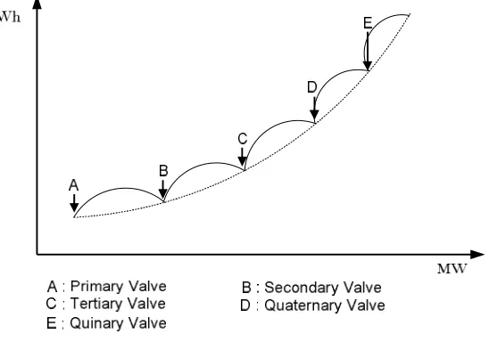
For more rational and precise modeling of fuel cost function, the above expression of cost function is to be modified suitably. The generating units with multi-valve steam turbines exhibit a greater variation in the fuel cost functions [10]. The valve opening process of multi-valve steam turbines produces a ripple-like effect in the heat rate curve of the generators. These “valve-point effects” are illustrated in Fig. 1.
The significance of this effect is that the actual cost curve function of a large steam plant is not continuous but more important it is non-linear. The valve-point effects are taken into consideration in the ELD problem by superimposing the basic quadratic fuel-cost characteristics with the rectified sinusoid component as follows:
n i i i i i i i i i i n i iT
F
P
a
P
b
P
c
e
f
P
P
F
1 min , 2 1sin
)
where FT is total fuel cost of generation in ($/hr) including valve point loading, ei, fi are fuel cost coefficients of the i th generating unit reflecting valve-point effects.
Fig. 1 Valve-point effects
III. DIFFERENTIAL EVOLUTION (DE) ALGORITHM
Differential evolution (DE) developed by Storn and Price [13] is a population based evolutionary computation technique, capable of handling non-differentiable, non-linear and multi-modal objective functions. Due to its simple but powerful and straightforward features, it is very attractive for resolving the non-convex global optimization problems. In DE, the fitness of an offspring competes one-to-one with that of the corresponding parent. This one-to-one competition will give rise to a faster convergence rate than other EAs. In addition, only a few control parameters are required in comparison with other computing heuristic optimization meth ods [14]. The basic algorithm of DE typically consists of four phases: 1) initialization, 2) mutation, 3) cros sover, and 4) selection phases. The mutation and crossover are used to generate new individuals, and the selection then determines that the individuals will survive into the next generation. The performance of DE algorithm usually depends on three parameters, i.e., population size NP, mutation factor MF, and crossover rate CR [13, 14].
A brief description of different steps of DE algorithm is given below:
3.1. Initialization
The population is initialized by randomly generating individuals within the boundary con straints
D
j
N
i
X
X
rand
X
X
p
j j
j ij
,
,
2
,
1
;
,
,
2
,
1
*
max minmin 0
(6)
3.2. Mutation
As a step of generating offspring, the operations of ‘mutation’ are applied. ‘Mutation’ occupies quite an
important role in the reproduction cycle. The mutation operation creates mutant vectors
X
i'kby perturbing arandomly selected vector
X
ak with the difference of two other randomly selected vectorsX
bk andX
ck at kth iteration as per following equation.
p k c k b k a k iN
i
X
X
F
X
X
,
,
2
,
1
'
(7)where
X
i'kis the newly generated ith population set after performing mutation operation at kthiteration;X
ak,X
bkandk c
X
are randomly chosen vectors at kth iteration
(
1
,
2
,
,
N
p)
anda
b
c
i
.k a
X
,X
bk andX
ckare selected for each new parent vector.]
2
,
0
[
F
is known as ‘scaling factor’ used to control the amount of perturbation in the mutation process and improve convergence. Many schemes of creation of a candidate are possible. Here strategy 1 has been mentioned in the algorithm.3.3. Crossover
Crossover represents a typical case of a ‘genes’ exchange. The parent vector is mixed with the mutated vector to create a trial vector, according to the following equation:
otherwise
X
q
j
or
Cr
j
rand
if
X
X
k i k ij k i' " (8)
where i=1,2,…, Np ; j=1, …, D.
X
ijk,
X
ij'k,
and
X
ij"k are the jth individual of ith target vector,mutant vector, and trial vector at kth iteration, respectively. q is a randomly chosen index
(j = 1, 2, …, D) that guarantees that the trial vector gets at least one parameter from the mutant vector even if Cr =0. Cr = [0, 1] is the ‘Crossover constant’ that controls the diversity of the population and aids thealgorithm to escape from local optima.3.4. Selection
Selection procedure is used among the set of trial vector and the updated target vector to choose th e best. Each solution in the population has the same chance of being selected as parents. Selection is realized by comparing the objective function values of target vector and trial vector. For minimization problem, if the tr ial vector has better value of the objective function, then it replaces the updated one as:
otherwise
X
X
f
X
if
X
X
k i k i k i k i k i)
(
" " 1 (9)where
X
ik1 is the ith population set obtained after selection operation at the end of kth iteration, to be used as parent population set (in ith row of population matrix) in next iteration (k +1 th).IV. MODIFIED DIFFERENTIAL EVOLUTION
4.1. Scaling factor F
In the initial DE, the scaling factor F in (7) is constant during the optimization process and F takes values in the range [0, 2]. However, no optimal choice of F has been proposed in the bibliography for DE. All the studies used an empirically derived value, and in most cases F varies from 0.4 to 1. This means F is strongly problem-dependent and the user should choose F carefully after some trial and error tests. In this section, F is varied randomly within some specified range, as follows:
F
a
b
rand
i[
0
,
1
]
(10)where a and b are positive and real-valued constants, the sum of a and b is less than 1,
rand
i[
0
,
1
]
denotes a uniformly distributed random value in the range [0, 1].Consequently, F is different for each generation, and the computation of F by (10) is effective when the optimal value of F is difficult to be determined for complicated problems like ELD.
4.2. Selection scheme
In the original DE, the trial vector or offspring
X
i"k is compared with the target vectorX
ik, whose index is the same as the running index i, using (9). In the modified DE algorithm, the trial vector is compared with the nearest target vector in the sense of Euclidean distance. This comparison scheme is employed in the crowding DE algorithm for multimodal function optimization. By this scheme, as the optimization proceeds, the individuals are scattered and gathered around the local optimal points. However, in this section, only global optimization is considered, and if there is no improvement of the optimal value during a predefined number of generations, then the comparison scheme is changed to that of the original DE.Therefore, in the initial period of optimization, the DE algorithm explores to find not only global but also local optima, and in the later stage, it searches only for the global optima with greedy selection scheme.
4.3. Auxiliary set
In the selection of the next generation individual, if the trial vector is worse than the target vector, then the trial vector is discarded. To enhance the explorative search and the diversity of the population, an auxiliary set is employed. The auxiliary set Pa has the same population size NP, and the initialization process is the same as that of the main set, using (6). At each generation, if the trial vector
X
i"k when compared with the corresponding target vector in the main set is found to be worse than its target vector, then the rejected trialvector is compared with the point
Z
ik with the same running index i in the auxiliary set Pa. If
k i ki
f
Z
X
f
"
, thenX
i"k replacesZ
ik.To use the solutions in Pa, after a predefined number of generations, several of the worst solutions in the main set are periodically replaced with the best ones in the auxiliary set by comparing the objective function value.
4.4. Treatment of constraints
Most optimization problems in the real world have constraints to be satisfied. One common approach to deal with constraints is to penalize constraint violations using an appropriate penalty function. In this approach, considerable effort is required to tune the penalty coefficients. In this section, three selection criteria are used to handle the constraints of the ELD problem:
1. If two solutions are in the feasible region, then the one with the better fitness value is selected.
2. If one solution is feasible and the other is infeasible, then the feasible one is selected.
It should be noted that the final (best) solution provided by MDE is accepted only if it is feasible; otherwise, the execution of MDE algorithm is repeated.
4.5. Handling of integer variables
DE in its initial form is a continuous variables optimization algorithm, and was extended to mixed variables problems. During the evolution process, the integer variable is treated as a real variable, and in evaluating the objective function, the real value is transformed to the nearest integer value as follows:
f
f
(
Y
)
:
Y
y
j (11)where,
'
continuous
is
if
),
(
INT
integer
is
if
,
j j
j j
j
x
x
x
x
y
(12)where INT (xj) function gives the nearest integer to xj, and the solution vector is
x
x
1,
x
2,
,
x
D
.V. SIMULATION RESULTS
To verify the feasibility and performance efficiency of applying MDE algorithm to solve ELD with taking the effect of valve ripples into consideration, several cases were tested and investigated. Among of these, two cases will be presented. The proposed MDE algorithm is applied to solve both the six-unit and fifteen-unit system with considering valve-point effects and transmission losses.
Test Case 1: 6-unit system
The system consists of six thermal generating units with valve point effects. The total load demand on the system is 1263 MW. The parameters of all thermal units are presented in Table 1 [9].
Table 1.Generating units capacity and coefficients (6-units)
Unit
min
i
P
(MW)P
imax(MW)a b c e f
1 100 500 0.0070 7.0 240 300 0.035
2 50 200 0.0095 10.0 200 200 0.042
3 80 300 0.0090 8.5 220 200 0.042
4 50 150 0.0090 11.0 200 150 0.063
5 50 200 0.0080 10.5 220 150 0.063
6 50 120 0.0075 12.0 190 150 0.063
0150
.
0
0002
.
0
0008
.
0
0006
.
0
0001
0
0002
.
0
0002
.
0
0129
.
0
0006
.
0
0010
.
0
0006
0
0005
.
0
0008
.
0
0006
.
0
0024
.
0
0000
.
0
0001
0
0001
.
0
0006
.
0
0010
.
0
0000
.
0
0031
.
0
0009
0
0007
.
0
0001
.
0
0006
.
0
0001
.
0
0009
.
0
0014
0
0012
.
0
0002
.
0
0005
.
0
0001
.
0
0007
.
0
0012
0
0017
.
0
.
.
.
.
.
.
B
ij
B
0i
1
.
0
e
3
0
.
3908
0
.
1297
0
.
7047
0
.
0591
0
.
2161
0
.
6635
B
00
0
.
0056
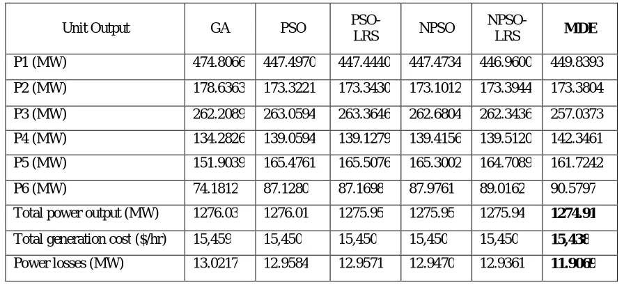
The obtained results for the 6-unit system using the MDE method are given in Table 2 and the results are compared with other methods reported in literature, including GA, PSO, PSO-LRS, NPSO, and NPSO-LRS [11]. It can be observed that MDE can get the total generation cost of 15,438 ($/hr) and power losses of 11.9069 (MW), which is the best solution among all the methods. Note that the outputs of the generators are all within the generator’s permissible output limit. A convergence characteristic of six-generator system is shown in Fig. 2.
Table 2. Comparison of the best results of each methods (PD = 1263 MW)
Unit Output GA PSO
PSO-LRS NPSO
NPSO-LRS MDE
P1 (MW) 474.8066 447.4970 447.4440 447.4734 446.9600 449.8393
P2 (MW) 178.6363 173.3221 173.3430 173.1012 173.3944 173.3804
P3 (MW) 262.2089 263.0594 263.3646 262.6804 262.3436 257.0373
P4 (MW) 134.2826 139.0594 139.1279 139.4156 139.5120 142.3461
P5 (MW) 151.9039 165.4761 165.5076 165.3002 164.7089 161.7242
P6 (MW) 74.1812 87.1280 87.1698 87.9761 89.0162 90.5797
Total power output (MW) 1276.03 1276.01 1275.95 1275.95 1275.94 1274.91
Total generation cost ($/hr) 15,459 15,450 15,450 15,450 15,450 15,438
Power losses (MW) 13.0217 12.9584 12.9571 12.9470 12.9361 11.9069
Test Case 2: 15-unit system
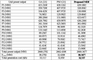
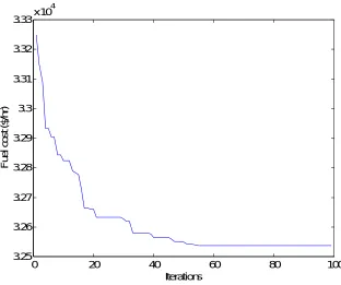
This system consists of 15 generating units and the input data of 15-generator system are given in Table 3 [9]. Transmission loss B-coefficients are taken from [21]. In order to validate the proposed MDE method, it is tested with 15-unit system having non-convex solution spaces, and the load demand is 2630 MW.
with the equality and inequality constraints by using the proposed constraint-handling approach. A convergence characteristic of fifteen-generator system is shown in Fig. 3.
Table 3.Generating units capacity and coefficients (15-units)
Unit Pmin (MW) Pmax (MW) a b c e f
1 150 455 0.000299 10.1 671 100 0.084
2 150 455 0.000183 10.2 574 100 0.084
3 20 130 0.001126 8.8 374 100 0.084
4 20 130 0.001126 8.8 374 150 0.063
5 150 470 0.000205 10.4 461 120 0.077
6 135 460 0.000301 10.1 630 100 0.084
7 135 465 0.000364 9.8 548 200 0.042
8 60 300 0.000338 11.2 227 200 0.042
9 25 162 0.000807 11.2 173 200 0.042
10 25 160 0.001203 10.7 175 200 0.042
11 20 80 0.003586 10.2 186 200 0.042
12 20 80 0.005513 9.9 230 200 0.042
13 25 85 0.000371 13.1 225 300 0.035
14 15 55 0.001929 12.1 309 300 0.035
15 15 55 0.004447 12.4 323 300 0.035
Table 4. Best solution of 15-unit systems (PD = 2630 MW)
Unit power output GA [21] PSO [21] Proposed MDE
P1 (MW) 415.3108 439.1162 439.1803
P2 (MW) 359.7206 407.9729 328.0043
P3 (MW) 104.4250 407.9729 130.0000
P4 (MW) 74.9853 129.9925 129.8645
P5 (MW) 380.2844 151.0681 433.6473
P6 (MW) 426.7902 459.9978 436.2364
P7 (MW) 341.3164 425.5601 361.6902
P8 (MW) 124.7876 98.5699 82.3329
P9 (MW) 133.1445 113.4936 62.2636
P10 (MW) 89.2567 101.1142 81.3096
P11 (MW) 60.0572 33.9116 46.4963
P12 (MW) 49.9998 79.9583 73.7417
P13 (MW) 38.7713 25.0042 25.0083
P14 (MW) 41.4140 41.4140 15.5043
P15 (MW) 22.6445 36.6140 15.0680
Total power output (MW) 2668.2782 2662.4306 2660.3477
PLoss (MW) 38.2782 32.4306 30.3477
Fig. 2 Convergence characteristic of six-generator system
Fig. 3 Convergence characteristic of fifteen-generator system
0 20 40 60 80 100 1.5435
1.544 1.5445 1.545 1.5455 1.546 1.5465x 10
4
Iterations
F
u
e
l
c
o
s
t
($
/h
r)
0 20 40 60 80 100
3.25 3.26 3.27 3.28 3.29 3.3 3.31 3.32 3.33x 10
4
Iterations
F
u
e
l
c
o
s
t
($
/h
VI. CONCLUSION
In this paper, a modified differential evolution (MDE) algorithm has been proposed, developed, and successfully applied to solve ELD problem with valve-point effects. The ELD problem has been formulated as a constrained optimization problem where an objective function has been considered to minimize the total generation cost. The proposed approach has been tested and examined on two different test systems. The simulation results demonstrate the effectiveness and robustness of the proposed algorithm to solve ELD problem. Moreover, the results of the proposed MDE algorithm have been compared to those reported in the literature. The comparison confirms the effectiveness and the superiority of the proposed MDE approach over the heuristic techniques in terms of solution quality.
REFERENCES
[1] A. J Wood, B. F. Wollenberg, Power Generation, Operation, and Control, 2nd ed., John Wiley and Sons, New York, 1996.
[2] Z. X. Liang, J. D. Glover, “A Zoom Feature for a Dynamic Programming Solution to Economic Dispatch Including Transmission Losses”, IEEE Trans. on Power Systems, vol. 7, no. 2, pp. 544-550, May 1992.
[3] C. L. Chiang, “Improved Genetic Algorithm for Power Economic Dispatch of Units with Valve-Point Effects and Multiple Fuels”, IEEE Trans. Power Systems, vol. 20, no. 4, pp. 1690-1699, 2005.
[4] W. M. Lin, F. S. Cheng, M. T. Tsay, “An Improved Tabu Search for Economic Dispatch with Multiple Minima”, IEEE Trans. Power Systems, vol. 17, no. 1, pp. 108-112, 2002.
[5] K. P. Wong, C. C. Fung, “Simulated Annealing Based Economic Dispatch Algorithm”, Proc. Inst. Elect. Eng. C, vol. 140, no. 6, pp. 509-515, 1993.
[6] K. Y. Lee, A. Sode-Yome, J. H. Park, “Adaptive Hopfield Neural Network for Economic Load Dispatch”, IEEE Trans. Power Systems, vol. 13, no. 2, pp. 519-526, 1998.
[7] N. Sinha, R. Chakrabarti, P. K. Chattopadhyay, “Evolutionary Programming Techniques for Economic Load Dispatch”, IEEE Trans. Evolutionary Computation, vol. 7, no. 1, pp. 83-94, 2003.
[8] H. T. Yang, P. C. Yang, C. L. Huang, “Evolutionary Programming Based Economic Dispatch for Units with Non-Smooth Fuel Cost Functions”, IEEE Trans. Power Systems, vol. 11, no. 1, pp. 112-118, 1996.
[9] Z. L. Gaing, “Particle Swarm Optimization to Solving the Economic Dispatch Considering the Generator Constraints”, IEEE Trans. Power Systems, vol. 18, no. 3, pp. 1187-1195, 2003.
[10] J. B. Park, K. S. Lee, J. R. Shin, K. Y. Lee, “A Particle Swarm Optimization for Economic Dispatch with Non-Smooth Cost Functions”, IEEE Trans. Power Systems, vol. 20, no. 1, pp. 34-42, 2005.
[11] A. I. Selvakumar, K. Thanushkodi, “A New Particle Swarm Optimization Solution to Nonconvex Economic Dispatch Problems”, IEEE Trans. Power Systems, vol. 22, no. 1, pp. 42-51, Feb. 2007.
[12] M. Vanita, K. Thanushkodi, “An Efficient Technique for Solving the Economic Dispatch Problem using Biogeography Algorithm”, European Journal f Scientific Research, vol. 50, no. 2, pp. 165-172, 2011.
[13] R. Storn, K. Price, “Differential Evolution a Simple and Efficient Heuristic for Global Optimization over Continuous Spaces”, J. Global Optim., vol. 11, no. 4, pp. 341-359, 1997.
[14] K. Price, R. Storn, J.A. Lampinen, Differential Evolution: A Practical Approach to Global Optimization, Springer, Berlin, Heidelberg, 2005. [15] J.P. Chiou, “A Variable Scaling Hybrid Differential Evolution for Solving Large-Scale Power Dispatch Problems”, IEE Proceedings – Generation, Transmission, and Distribution, vol. 3, no. 2, pp. 154-163, 2009.
[16] M. Vanita, K. Thanushkodi, “Solution to Economic Dispatch Problem by Differential Evolution Algorithm Considering Linear Equality and Inequality Constraints”, International Journal of Research and Reviews in Electrical and Computer Engineering, vol. 1, no. 1, pp. 21-26, 2011. [17] L. Lakshminarasimman, S. Subramanian, “Short-Term Scheduling of Hydrothermal Power System with Cascaded Reservoirs by using Modified Differential Evolution”, IEE Proceedings – Generation, Transmission and Distribution, vol. 153, no. 6, pp. 693–700, November 2006. [18] Georgilakis PS, “Differential evolution solution to the market-based transmission expansion planning problem”, Proc Mediterranean Conference Power Generation Transmission Distribution Energy Conversion (MedPower 2008), Thessaloniki, Greece, November 2-5, 2008. [19] G.Y. Yang, Z.Y. Dong, K.P. Wong, “A Modified Differential Evolution Algorithm with Fitness Sharing for Power System Planning”, IEEE Trans. Power Systems, vol. 23, no. 2, pp. 514–522, 2008.
[20] Ganga Reddy Tankasala, ”Artificial Bee Colony Optimisation for Economic Load Dispatch of a Modern Power System”, International Journal of Scientific & Engineering Research, vol. 3, no. 1, pp. 1-6, 2012.
[21] G. Shabib, A.G. Mesalam, A.M. Rashwan, “Modified Particle Swarm Optimization for Economic Load Dispatch with Valve-Point Effects and Transmission Losses”, Current Development in Artificial Intelligence, vol. 2, no. 1, pp. 39-49, 2011.
BIOGRAPHY
Hardiansyah was born on February 27, 1967 in Mempawah, Indonesia. He received the B.S. degree in Electrical