Reducing Computational Load for Mixed Integer Linear Programming:
An Example for a District and an Island Energy System
Timo Kannengießer,1,4 Maximilian Hoffmann,1,4 Leander Kotzur,1 Peter Stenzel,1 Peter Markewitz,1 Fabian Schuetz,² Klaus Peters,² Stefan Nykamp,3 Detlef Stolten1, 4 and Martin Robinius1
1Institute of Electrochemical Process Engineering (IEK-3), Forschungszentrum Juelich GmbH,
Wilhelm-Johnen-Str., 52428 Juelich, Germany, +49 2461 61-8732, [email protected]
2 Westnetz GmbH, Florianstraße 15-21, 44139 Dortmund, Germany
3 Innogy SE, Kruppstraße 5, 45128 Essen, Germany
4 Chair for Fuel Cells, RWTH Aachen University, c/o Institute of Electrochemical Process Engineering
(IEK-3), Forschungszentrum Juelich GmbH, Wilhelm-Johnen-Str., 52428 Juelich, Germany
Abstract
The complexity of Mixed-Integer Linear Programs (MILPs) increases with the number of nodes in energy system mod-els. An increasing complexity constitutes a high computational load that can limit the scale of the energy system model. Especially in microgrid optimisation problems with multiple buildings and energy systems with a number of rival supply, distribution and storage technologies, methods are sought to reduce this complexity. In this paper, we present a new 2-Level Approach to MILP energy system models that determine the system design through a combination of continuous and discrete decisions. On the first level, data reduction methods are used to determine the discrete design decisions in a simplified solution space. Those decisions are then fixed, and on the second level the full dataset is used to extract the exact scaling of the chosen technologies. The performance of the new 2-Level Approach is evaluated for a case study of an urban energy system with six buildings and an island system based on a high share of renewable energy technologies. The results of the studies show a high accuracy with respect to the total annual costs, chosen system structure, installed capacities and peak load with the 2-Level Approach compared to the results of a single level optimi-zation. The computational load is thereby reduced by more than one order of magnitude, while a significantly higher accuracy is reached in comparison to the common time series aggregation approach.
Keywords: MILP, District Optimization, Energy system model, Time series aggregation, Typical periods
1
Introduction
Urban districts are in search of strategies to reduce greenhouse gas (GHG) emissions. The strategies should be cost- and environmentally-optimal solutions for a future district energy supply system. Microgrids have the potential to contribute to GHG reductions in urban districts because of their higher efficiency due to energy utilization synergies [1] .
In the literature, microgrids are usually divided into microgrids with grid connection to the macrogrid and island microgrids without a connection to a higher grid level [2-4]. A microgrid can include multiple residential and commercial buildings with specific electricity, heating and cooling demands. These are supplied by conventional technologies like boilers, distributed energy resources (DERs) such as photovoltaic (PV), en-ergy storages technologies like batteries, and different enen-ergy distribution grids for electricity, natural gas and district heating [5-7]. The advantage of microgrids is the cost-optimal operation of supply technologies through exchanging the energy between the buildings and storing it [8].
1.1 The complexity of microgrid supply system optimization
Determining the optimal design and operation of microgrids is a complex task that imposes demanding requirements on computational resources and mathematical solvers. Different mathematical approaches, such as Mixed-Integer Linear Programming (MILP) [2, 4, 6, 9-20], Mixed-Integer Non-Linear Programming (MINLP) [21, 22] and metaheuristic approaches [3, 23-28] are used to determine the optimal design or operation of microgrid energy supply systems. The advantage of mathematical programming like MILP to metaheuristics is that the distance to the global optimum can be determined, which increases the quality of
the results. On the other hand, the computing time is high with MILP, as shown in Morvaj et al. [16] and, especially for Mixed Integer Non-Linear Programming [22] metaheuristic approaches, allows for a higher spatial resolution compared to mathematical programming because of lower complexity, but the global op-timum is not guaranteed.
Mehleri et al. [6] developed a MILP model to design and operate a cost-optimal energy supply system for a five-building neighbourhood in Greece. The conceptualized microgrid contains a boiler, a combined heat and power plant (CHP), photovoltaic (PV) and thermal storage capacity, along with an electrical and natural gas macrogrid connection, as well as a local district heating network. A metaheuristic approach was devel-oped by Prousch et al. [29] to schedule the operation of heat pumps, CHP units and electric vehicles in a district with 69 nodes, which includes 10,074 households with commercial and residential buildings. Olivares et al. [22] present a MINLP approach for the operation of microgrids. A non-linear approach was used to manage the reactive power in the distribution grid, such that the model complexity was higher than in a linear mathematical program, as in a MILP model.
Furthermore, Morvaj et al. [15] present a multi-objective MILP approach to optimize the economic, environmental and technical criteria and compare it with a bi-level as well as a combined approach of MILP and bi-level optimization. The optimal design and operation were focused on five residential buildings by adding grid constraints. These constraints are used in terms of linearized AC power flow for the MILP and nonlinear AC power flow for the bi-level approach. In the combined approach, linear and nonlinear AC power flow is used in order to check the accuracy of the linearized results. In comparison to the MILP approach, the bi-level approach shows better solving performance, while the optimality is not guaranteed. The com-bined approach has the best overall performance for optimality, accuracy and solving performance. Another MILP model was developed by Omu et al. [17] and applied in a case study in Southern England in a six-building case study to investigate an electrification and standalone CHP scenario with different degrees of decentralization.
1.2 State of the art of complexity reduction
Systematic reduction of model complexity is often used to solve design and operation optimization problems on different energy system levels, e.g., reducing the complexity through decomposition, as in Falke et al. [25], to determine the cost- and environmentally-optimal technology configuration of a microgrid on the basis of a metaheuristic approach. The optimization problem was decomposed into three subproblems to reduce the computational complexity and to plan the heating network, generation and renovation process, as well as the simulation of the operation. Another way to reduce the computing time is to decrease the spatial resolution [30-32]. Fazlollahi et al. [30] developed an approach to cluster data provided by Geographic In-formation Systems (GIS) using the k-means clustering technique. With this approach, it was possible to reduce the number of nodes from 475 to 13.
Often, less than 20 individual buildings are regarded in MILP microgrid models [6, 9, 10, 15, 17, 19]. Aside from the number of buildings, the number of time steps directly influences the size of the mathematical model and increases its complexity [15].
A common strategy to decrease the complexity is to decrease the temporal resolution by averaging time series to typical periods [6, 9, 11, 12, 33, 34] or to cluster them to typical periods [2, 12, 20, 35-37]. For example, Zhou et al. [34] developed a MILP model for determining the optimal design as well as the operation of technologies. The hourly resolved time series were averaged to one typical day for every month, so that the temporal resolution was reduced to 288 time steps. Averaged periods successfully reduce the computing time but lead to an inferior representation of the time series [9, 36]. Thus, the clustering of time series is preferred for reducing optimization complexity. Kotzur et al. [36] compare different clustering meth-ods and reveal effects on the cost, design and operation of different energy systems in detail.
Although time series aggregation is promising, it still has the drawback that a system design based on the reduced time series data is not guaranteed to be feasible for the full original time series. The underestimation of storage technologies and peak loads, as shown in Kotzur et al. [36], is a problem due to the lack of modelled time steps.
1.3 Research objective
In this paper, we present a new approach to decrease the complexity of MILP optimization models by split-ting the optimization problem into two levels. The new 2-Level Approach is developed for MILP models for the design and operation of energy systems. On the first level, the structure of the energy system is determined with time series aggregation. The scaling of the chosen technologies and the operation optimization is conducted on the second level.
In section 2, we present the applied methodology of the energy system optimization, as well as a detailed description of the new 2-Level Approach. In section 3 and 4, two case studies and their general input time series data, which is required for microgrid optimization, are presented. The first is a case study with six buildings in a spatially-distributed network and the second is a single-node island system with a high share of renewable energy and limited fossile fuels-based electricity production. These case studies were chosen to investigate the impact of the proposed 2-Level Approach on both distributed energy systems with a number of identical units in different places and single-node energy systems with a number of rival, but different supply and storage technologies and a focus on the seasonal storage capacity usually required by highly renewable energy systems. In section 5, the results of the case studies are analyzed and discussed.
2
Methodology
In the following sections the optimization model (section 2.1), the new 2-Level Approach (section 2.2) and the scenario definition for both case studies (section 2.3) are described.
2.1 Energy system optimization model formulation
The energy system models are formulated as MILP, as presented in Welder et al. [39] with the FINE optimization framework [40]. Furthermore, we applied the time series aggregation module (TSAM) [41] for the new 2-Level Approach based on the FINE framework. The objective function of the optimization models is to minimize their total annualized cost (TAC). A detailed formulation of the energy system model can be found in Welder et al. [40].
The cost structure of the technology portfolio is represented by fix and capacity-related CAPEX and OPEX costs. The fixed costs are modelled with a binary variable that determines if the technology is installed in the microgrid energy supply system or not.
In the first case study, every building in the microgrid is represented by a node. Hence, the spatial resolution depends on the number of investigated buildings. In the second case study, all technologies are located in one node and have a limited capacity for a supply based on fossil fuels. The temporal resolution is one hour and depicts one year with 8,760 time steps.
As the mathematical solver, we used Gurobi 8.0 (first case study) and Gurobi 8.1 (second case study). Pyomo is used as the modeling language.
2.2 2-Level Optimization Approach
In the following, a new 2-Level Approach is presented to reduce the complexity of optimization problems and increase the accuracy of the results compared to time series aggregation alone.
Optimization specifications
· Time series data · Techno-economic
parameter
TSA specifications
· Typical periods · Cluster method
Microgrid energy system model with FINE
Clustering in FINE with TSAM
Optimization with FINE (Typical Periods)
cap1, op1
bin1
Optimization with FINE (Full Time Series)
Microgrid energy system model with FINE (Fixed Binaries)
bin2=bin1, cap2, op2
1
st L
ev
el
2
n
d L
ev
el
TSA: Time Series Aggregation
TSAM: Time Series Aggregation Module [41]
FINE: Framework for Integrated Energy System Assessment [40]
cap: Capacity of installed technologies
op: Optimal operation of technologies
bin: Binary variable for technologies
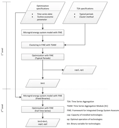
Figure 1. Workflow of 2-Level Approach.
On the first level, the optimization specifications are defined with time series data such as weather condi-tions, as well as the load profiles and techno-economic parameters of the considered technologies to build the microgrid energy system model in FINE. Furthermore, the time series aggregation (TSA) specifications with typical periods and the cluster method are specified. The storage operation between the typical periods is enabled by a superposition of system states [42].The typical periods represent the full time series by clustering a set of similar periods around a set of typical periods (typical days). In this study, we use different numbers of typical days to represent the full time series. A low number of typical days (e.g., 5 typical days) typically leads to better computing performance compared to a high number (e.g., 40 typical days). On the other hand, the accuracy of the optimization results decreases with a decreasing number of typical days [36].
Different clustering methods such as k-means, k-medoids or hierarchical aggregation are common to cluster time series. For the first level, a hierarchical clustering algorithm [43] is used, as it is easily reproducible and maintains a higher variance of the input time series by representing the clusters with their medoid.
are determined, with only the technology structure of the microgrid energy supply system as binaries is used for the second level.
On the second level, the installed capacities of fixed technologies (technology scaling) and the optimal system operation are determined with the full time series based on the set of binary variables (fixed tech-nology structures) divided from the aggregated optimization on the first level. Hence, the MILP is reduced, with the given binaries, to a linear program. As a result, the optimal design and operation of energy supply system with higher accuracy compared to a time series aggregation is obtained because of the optimization with the full time series in the second level of the 2-Level Approach.
Furthermore, it should be mentioned that the proposed method could also be applied to components with piecewise linear cost functions, i.e., with more than one binary variable per component. The
2.3 Scenario definition
To validate the methodology, the design and operation of the energy system is first determined by the new 2-Level Approach and then by a single problem with aggregated time series. These are compared to the reference case, which is computed with a full-time series, and no aggregation techniques are applied. For the 2-Level Approach and the time series aggregation, typical periods consisting of 5, 10, 20 and 40 typical days are considered in hourly resolution (see Table 1).
Reference Time series aggregation 2-Level Approach
1st Level MILP MILP MILP
Full-Time Series Typical Periods Typical Periods
2nd Level - - LP
- - Full-Time Series
Table 1. Overview of optimization approach and considered time series in 2-Level Approach, time series ag-gregation and the reference case.
The scenarios of both case studies are totally identical in order to maintain consistency and enable a com-parison between small single-node models with a high relevance of seasonal storage and more complex and distributed energy systems. This means that on the first level of the approach, the input data is sorted into daily duration curves and aggregated with Ward’s [44] hierarchical clustering algorithm for 5, 10, 20 and 40 typical days (i.e., clusters). The energy systems of both case studies are individually optimized for each of the three defined scenarios, e.g., the 2-Level Approach, the time series aggregation and the refer-ence case. The results of the total annual costs (TAC), computing time and installed capacities are used to compare the scenarios.
3
First case study – Urban energy system
An exemplary district is investigated with six multi-family houses and six households in every individual building. The district is located in Germany. The buildings have similar building parameters and are con-nected by an electricity grid and a natural gas network. In section 3.1, we will give an overview of the un-derlying data, such as the total energy demand of the considered district. Furthermore, the technology port-folio is presented in section 3.2. Finally, in section 3.3 scenarios are defined that determine the available technology portfolio in the district.
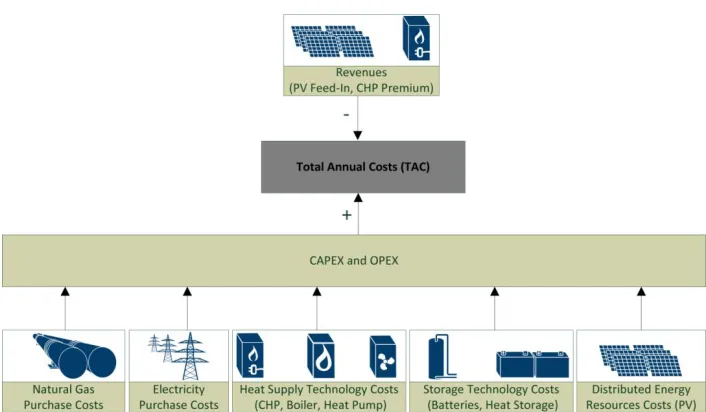
Figure 2. Composition of total annual costs in the microgrid optimization model.
3.1 Data basis
In the following section, the preprocessing of the time series data for the microgrid optimization model is shown.
For the simulation of the heat load and PV generation profiles, the weather data of the test reference year (TRY) by the German Weather Service (DWD) for climate region 5 (Lower Rhine Westphalian Bay and Emsland) are used. The weather data is based on the period from 1988 to 2007. Different TRY data are available for mean, extreme cold and warm weather years. This work considers the weather year that cor-responds to the mean temperature.
A stochastic bottom-up simulation model implemented in Python is used to determine the domestic electrical demand. The model based on the CREST Demand Model [45-47] simulates the domestic electrical demand depending on the number of residents, the number of apartments and the individual user behavior of inhab-itants. In addition to light bulbs, LED and halogen lamps were integrated into the model on the basis of statistical data for Germany [48]. The user behaviour of the inhabitants is determined by a probability distri-bution of the devices used in the households. The temporally-resolved use of the devices is modelled by transition probabilities that are determined by first order Markov chains.
The domestic heating demand for buildings is determined with a 5R1C model that was modelled and imple-mented in Python as per Schuetz et al. [21] and is based on the EN ISO 13799. The demand is simulated in a building depending on the outside temperature, solar radiation, wind and building parameters by optimizing the living space temperature between two limit temperatures (21°C-24°C). It is assumed that the domestic heating is only used during the typical North European heating period between 1st of October and 30th of April. The energy requirement for the supply of hot water is not considered.
The PV generation potential is site-specifically calculated with PVLIB Python [49] for the district. For the calculation of the PV generation profiles, it was assumed that all PV systems are constructed by modules of the type Hanwha HSL60P6-PA-4-250T, with a nominal power of 250 W. Each module is connected to an ABB MICRO-0.25-I-US inverter. The maximum installable capacity is determined depending on the availa-ble roof area. In Germany, roofs are often designed as saddle roofs, which means that their entire surface is usually distributed across two areas. The optimal installed PV capacity for a microgrid energy supply system is chosen by the microgrid optimization and is not part of the preprocessing.
The load profiles and demand characteristics are presented in the appendix.
3.2 Technology Portfolio
electricity generation, storage technologies and grids. Boilers, CHPs and heat pumps are options for fulfilling the heat demand of the buildings in the microgrid optimization. The electricity demand can be satisfied by CHPs and PV as DER, as well as by the purchase of electricity over the macrogrid. Storage technologies in the microgrid optimization include batteries and heat storage. The buildings in the microgrid optimization are connected with an electricity distribution grid and a natural gas network. The electricity grid allows an exchange of locally-produced electricity across the buildings. The natural gas network is required to supply boilers and CHPs with natural gas.
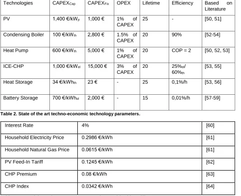
The cost structure of the considered technology portfolio is based on actual (the year 2017) technologies and energy prices, as well as the regulatory framework for grid feed-in of electricity in Germany (see Table 2 and Table 3). The grid feed-in is based on the regulatory framework of the German Renewable Energies Act (EEG) for PV and Combined Heat and Power Act (KWKG) for CHP. The electricity distribution grid and the natural gas network costs are not part of the optimization and it is assumed, that they are already in place.
Technologies CAPEXCap CAPEXFix OPEX Lifetime Efficiency Based on Literature
PV 1,400 €/kWp 1,000 € 1% of
CAPEX
25 - [50, 51]
Condensing Boiler 100 €/kWth 2,800 € 1.5% of CAPEX
20 90% [52-54]
Heat Pump 600 €/kWth 5,000 € 1% of
CAPEX
20 COP = 2 [50, 52, 53]
ICE-CHP 1,000 €/kWel 15,000 € 3% of
CAPEX
20 25%el/
60%th
[53, 55]
Heat Storage 34 €/kWhth 23 € - 25 0,1%/h [53, 56]
Battery Storage 700 €/kWhel 2,000 € - 15 0,01%/h [57-59]
Table 2. State of the art techno-economic technology parameters.
Interest Rate 4% [60]
Household Electricity Price 0.2986 €/kWh [61]
Household Natural Gas Price 0.0615 €/kWh [61]
PV Feed-In Tariff 0.1245 €/kWh [62]
CHP Premium 0.08 €/kWh [63]
CHP Index 0.0342 €/kWh [64]
Table 3. State of the art interest rate, energy prices and feed-in tariffs.
3.3 Results of the first case study
The installed capacities of the technologies are based on the microgrid optimization results for the reference case and are shown in Figure 3. A CHP is only installed in building 1 (bd1). The district’s largest heat storage is also built in building 1 to optimize the operation of the CHP. The second highest heating and electricity demand of all buildings in the district, as well as the peak electricity load in comparison to the other individual buildings, is located in building 1. Therefore, it is apparent that there is a correlation between the electricity peak load and the location of the CHP installation.
In buildings 2, 3, 4, 5 and 6 (bd2- bd6), the technology system design for the heat supply is similar. A natural gas boiler combined with a heat storage unit is chosen. A PV installation can be found in buildings 1, 2, 3 and 6. The reason for the missing PV in building 4 and 5 is the unfavorable roof orientation.
Figure 3. Installed capacities in buildings (bd) for reference case with full-time series.
In sections 3.3.1-3.3.4, the microgrid optimization will be executed with the time series aggregation ap-proach, as well as the new 2-Level Apap-proach, to compare the results with those from the reference case.
3.3.1 Investigation of total annual costs
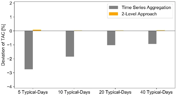
The TAC in the 2-Level Approach shows a low deviation of less than 0.1% related to the TAC of the refer-ence case, as shown in Figure 4. In the results of the time series aggregation, the deviation is higher in comparison to the 2-Level Approach for the analyzed different typical days. With an increasing number of typical days, the deviation of the time series aggregation related to the reference case decreases, but is still higher than in the 2-Level Approach. The 2-Level Approach shows a significantly lower deviation than the time series aggregation. For all typical periods, the 2-Level-Approach tends to slightly overestimate the TAC, whereas the time series aggregation tends to underestimate it. The reason for the underestimation of the TAC in the time series aggregation approach is the averaging effect caused by the clustering of time series data.
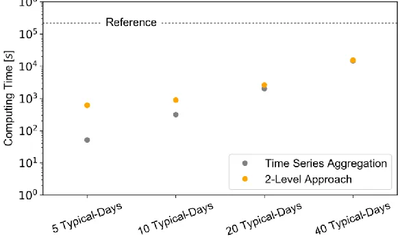
3.3.2 Investigation of computing time
The investigation of computing time runs on a Windows desktop PC with an Intel(R) Core(R) i7-6700K @4.00GHz and a Memory of 32 GB RAM.
Figure 5 shows a significantly lower computing time for the 2-Level Approach and the time series aggrega-tion related to the reference case. The 2-Level Approach results in a decrease in the computing time of between -99.72% for 5 typical days and -92.96% for 40 typical days compared to the reference case. The time series aggregation reduces the computing time by -99.97% for five typical days and -93.22% for 40 typical days.
The computing time of the first level in the 2-Level Approach is equal to the time series aggregation because it follows the same approach. The computing time is 51 seconds for 5 typical days, 315 seconds for 10 typical days, 2,017 seconds for 20 typical days and 14,754 seconds for 40 typical days. In addition to the time series aggregation in the first level of the 2-Level Approach, a full-time series optimization is running that results in an overall higher computing time for the 2-Level Approach than for the time series aggrega-tion. The second level of the 2-Level Approach is an LP problem. Thus, the computing time changes only slightly with a minimum of 556 seconds and maximum of 597 seconds for solving the second level.
Figure 5. Comparison of the computing time.
3.3.3 Investigation of the supply technologies
The microgrid optimization with full-time series (reference case), time series aggregation and the 2-Level Approach show the same technology structure. To fulfil the electricity and heating demand, the microgrid optimization opts for boilers, CHPs, heat storages and PV as supply technologies. The investigation of all installed supply technologies in the district is considered in the following sections.
3.3.3.1 Boiler
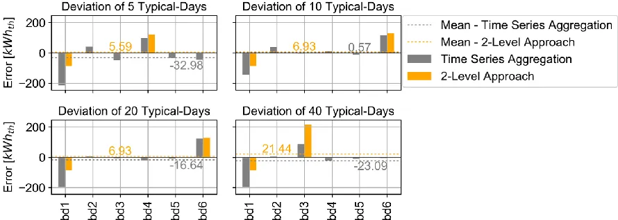
The mean deviation of the 2-Level Approach related to the reference case is low, with a maximum of -4.46 kWth in 40 typical days and a minimum of -0.12 kWth in 5 typical days. In the time series aggregation, the mean deviation decreases from -51.8 kWth in 5 typical days to -17.57 kWth in 40 typical days. Thus, the mean results show a significantly lower deviation in the 2-Level Approach than in the time series aggrega-tion.
Moreover, we can observe that the time series aggregation shows a similar pattern to that in the 2-Level-Approach with respect to the CHP-based capacity shifting. The installed capacities increase in building 1 and decrease in the building with the new CHP location. Additionally, there is a trend of high underestimation of boiler capacities in the buildings, which are not part of the changing CHP location. The underestimation of installed capacities decreases with an increasing number of typical days because of more detailed time series data.
Figure 6. Deviation of installed boiler capacities with the 2-Level Approach and time series aggregation in buildings (bd) compared to full time series.
3.3.3.2 CHP
As discussed in section 3.3.3.1, the CHP installation location changes between the reference case and the 2-Level Approach, as well as the time series aggregation (see Figure 7). In the case of 5 typical days, the installed CHP shifts from building 1 to building 4, while in the case of 10 and 20 typical days, from building 1 to building 6, and in the case of 40 typical days, from building 1 to building 3.
The mean deviation of the installed CHP capacities computed with the 2-Level Approach is 0.02 kWth for all typical days. The optimization with the time series aggregation results in a minimal deviation of -0.02 kWth for 5 typical days and a maximum of 0.39 kWth for 40 typical days.
A possible reason for the building shifting the CHP installation between the different typical days is that the difference in the TAC is not significant. Hence, its location does not affect the TAC. A further analysis is performed in order to investigate the TAC in relation to the location of the CHP in section 3.3.5.
Figure 7. Deviation of installed CHP capacities with 2-Level Approach and time series aggregation in build-ings (bd) compared to full time series.
3.3.3.3 Heat Storage
As described in the analysis of boilers and CHPs, the heat storage results also show a clear pattern of capacity shifting between the buildings on the different typical days, especially in the 2-Level Approach, as shown in Figure 8. In the case of 5 and 10 typical days, the installed heat storage capacities decrease in building 1 and increase in building 6, while in the case of 10 and 20 typical days, the installed capacities shift from building 1 to building 6. The possible reason for the same pattern of capacity shifting as in the CHP investigation is that the heat storage supports the operation of the CHP. The electricity generation costs with the CHP are, at 0.26 €/kWh, cheaper than purchasing electricity for 0.2985 €/kWh from the energy provider. Thus, the CHP is preferred by the optimizer to generate electricity, but the thermal energy of the CHP must be used to fulfil the heating demand or store heat in the storage, because an external chiller is not available for the CHP. Hence, the heat storage follows the CHP to buffer excess thermal energy. The reason for the other typical day's high deviation of heat storage capacities in 40 typical days is a result of the underestimation of boiler capacities in building 3 for 40 typical days, which does not influence the TAC of the energy supply system.
Figure 8. Deviation of installed heat storage capacities with the 2-Level Approach and time series aggrega-tion.
3.3.3.4 PV
As well as the 2-Level Approach, the time series aggregation meets the installed PV capacities in the refer-ence case for the different investigated typical periods. Thus, both approaches represent the installed PV capacities very well with no deviation from the reference case.
3.3.4 Investigation of peak load
The peak load is the maximum electrical load, which flows over the grid assets. In general, a transformer in a microgrid optimization is the connection between a district and a higher grid level (e.g. between a low voltage and a medium voltage grid). The load flow is divided into two directions: The top-down load flow with the electricity from higher grid level flows via the transformer to fulfil the electricity demand in the district, whereas the bottom-up load flow is defined as the flow from the district (lower) to the higher grid level via the transformer. Bottom-up load flow occurs when the locally-produced electricity (e.g., from PV, CHP) ex-ceeds the local electricity demand in the district. The peak load is essential to analyze the stress of the transformer. Furthermore, voltage issues may become relevant in real grids but are out of scope for this investigation. The peak load investigation is only applied to the electricity grid and not to the natural gas network.
The bottom-up peak load and the top-down peak load of the reference case is very well addressed with the 2-Level Approach, as shown in Figure 9. The time series aggregation underrepresents the peak load for the different typical days. Only in the case of 20 typical days in the bottom-up peak load is the result of the time series aggregation close to the reference case. The result is probably based on a coincidence, as it is worse with 40 typical days.
the smaller cluster. Also, it is possible to add peak periods to the time series aggregation, which leads to a more accurate solution. On the other hand, adding peak periods leads to an increase in optimization com-plexity and increasing computing time due to additional time periods.
Hence, the investigation shows that the 2-Level Approach is well suited to represent the bottom-up peak load and top-down peak load while the time series aggregation represents it insufficiently.
Figure 9. Bottom-up and top-down peak load flow of time series aggregation and 2-Level Approach compared to the reference case with full time series.
3.3.5 Impact analysis of fixed CHP position
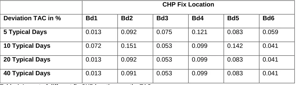
The investigation of CHPs in 3.3.3.2 showed that only one CHP was installed in one building in the analyzed microgrid energy supply system, but the building location of the CHP installation changes between the dif-ferent typical days. In the reference case, the CHP was installed in building 1. In the 2-Level Approach, the CHP was installed in building 4 for 5 typical days, in building 6 for 10 and 20 typical days, respectively, and in building 3 for 40 typical days. To investigate the impact of the changing installed CHP location for different typical days, an analysis was performed. In this analysis, the buildings with the installed CHP were fixed one after another to investigate the deviation of TAC related to the reference case. The results of the analysis are shown in Table 4. On the one hand, the table shows the location of the fixed installed CHP location in columns and, on the other hand, the deviation of the TAC related to the reference case for 5, 10, 20 and 40 typical days.
The analysis shows that the deviation of the TAC for different fixed CHP locations is low compared to the reference case with 0.013% to 0.151%. The lowest deviation of 0.013% can be reached if the CHP is fixed in building 1, which corresponds to the location of the reference case. The highest deviation of TAC is identifiable for a fixed CHP location in building 2, with 0.151% and 10 typical days. However, in general, all results with the fixed location of the CHP show low deviations compared to the reference case. Therefore, the impact of the different placements of CHPs on the TAC is low.
CHP Fix Location
Deviation TAC in % Bd1 Bd2 Bd3 Bd4 Bd5 Bd6
5 Typical Days 0.013 0.092 0.075 0.121 0.083 0.059
10 Typical Days 0.072 0.151 0.053 0.099 0.142 0.041
20 Typical Days 0.013 0.092 0.053 0.099 0.083 0.041
40 Typical Days 0.013 0.091 0.053 0.099 0.083 0.041
Table 4. Impact of different fix CHP locations on the TAC.
If the CHP is installed in building 1, which is the location of the reference case, there is no changing with respect to the installed capacities for boilers and heat storage. In the other cases of a fixed CHP location, there is a clear pattern that boiler capacities decrease and heat storage capacities increase in the building of the fixed CHP installation. Furthermore, in building 1, the boiler capacities increase, and the heat storage capacities decrease. The reason for increasing boiler capacities in building 1 is that the thermal capacities of the CHP are missing.
Figure 10. Changing capacities based on fixed CHP location.
4
Second case study – Island system
The second study focuses on the application of the presented 2-Level Approach on a simple single-node island system with two commodities, namely electricity and hydrogen. The island system consists of a wind farm, photovoltaics and a small backup plant as the energy supply and a single electricity demand. Moreo-ver, two alternative energy storage technologies are included: The first stores electricity directly using bat-teries, while the second uses electrolyzers and fuel cells to store the surplus energy from the electrical grid in hydrogen pressure vessels [65] using electrolysis.
4.1 Data basis
4.2 Technology portfolio
The detailed input parameters used for modeling the island system model can be taken from Table 5 and are derived from Kotzur et al. [42] with an interest rate of 4% per year for each component for consistency to the above presented case study. It is worth mentioning that only the wind farm, the photovoltaics, the electrolyzer and the fuel cell are modeled with binary variables according to a certain starting investment (named CAPEXFix in the tables) and fix operation costs (OPEXFix) depending on the decision whether these units are chosen (1) or not (0). In contrast to that, the backup plant, the battery and the hydrogen storage are modeled linearly since their overall costs only depend on their consumed commodity (gas with 20 ct/kWh in case of the backup plant) and their capacities respectively. This fairly simple layout is chosen to empha-size the big impact of the proposed 2-Level Approach on the computing time even for small systems while maintaining good results. Besides, a single-node model with a high share of renewable energy was chosen to highlight the impact of the proposed method on seasonal storages while neglecting balancing effects of multi-regional distribution grid modeling.
Figure 11. Technology portfolio of the island system.
CA P E XCap [€/ kW p ] CA P E XFix
[€] OP
E XCap [€/ kW p ] O P E XF ix [€] O P E XVar [€/ kW h] E ffi c ien c y [%] Charge E f-fi c ie nc y
[%] Dis
c ha rge E ffi c ien c y
[%] Sel
f-Di s -c ha rge
[%/h] Life
ti
m
e [
a
]
Photovoltaic 800 1,000 8 100 0 20
Wind Energy 1,000 100,000 20 2,000 0 20
Backup Plant 1,000 0 30 0 0.2 25
Electrolyzer 500 100,000 15 3,000 0 70 15
Fuel Cell 1,100 100,000 33 3,000 0 50 15
Battery 300 0 3 0 0 96 96 0.05 15
Hydrogen Storage
15 0 0 0 0 90 1 0 25
Table 5. Unit parameters of the island system derived from Kotzur et al. [42].
4.3 Results of the second case study
The following section focuses on the optimization results of the island system presented above. The follow-ing sections first investigate the total annual cost as the actual objective function of the optimization, the computing times to highlight the benefits of the 2-Level Approach followed by a detailed analysis of the component’s capacities within the different levels of the proposed approach.
The deviation of the total annual costs depending on the number of typical days and the level in which they are determined by the optimization, in comparison to the reference case that uses the full time series, as well as all four binaries as variables, is illustrated in Figure 12.
Figure 12. Deviation of total annual costs for different typical days compared to full time series.
As mentioned above, the optimization based on 5 or 10 typical days using hierarchical clustering of the daily duration curves leads to a negligence of the hydrogen technologies that ultimately ends up in higher total annual costs of the whole system after the second optimization. This can be reasoned by the fact that the clustering algorithm has a big impact on the smoothness and variance of the clustered input data. In the case of the first level of the optimization using 5 or 10 typical days this leads to an underestimation of the total variance of the input time series, which means that the time series is considered to be highly repetitive and the overall variance is not kept which has an impact on the design of surplus capacities. Since the fuel cell and the electrolyzer have a start investment of 100.000 € each before building any capacities at all, the optimization based on the aggregated time series turns out to be more profitable if the hydrogen storage technology is not chosen. Because of the fact that the binary variables from the first level of optimization are used as input parameters for the second level of optimization, the hydrogen technologies are not imple-mented as well when repeating the optimization with the full time series. This turns out not to be a sufficient assumption since the overall costs of the energy system based on batteries as the only storage technology exceeds the total annual costs of the reference case by approximately 7%.
20 typical periods seem to be sufficient to find the right combination of binary variables, which means that all technologies with binary variables, namely wind, PV and the hydrogen technologies, are chosen accord-ing to the reference case. This reduces the deviation of the total annual costs compared to the reference case to zero after the second level of optimization. This can also be observed for 40 typical days. However, it needs to be highlighted that in this case the deviation of the total annual costs after the first level of optimization is already far below 1% which raises the question if the second level of optimization is neces-sary at all in this case. Last but not least it needs to be stated that the number of clusters for finding a good set of binary variables is a highly non-trivial question and that it is not guaranteed that the set of binary variables found in the first level always remains the same when choosing more than 20 typical days. How-ever, the chance of finding the cost-optimal set of binary variables becomes more and more likely when increasing the number of typical days.
4.3.2 Investigation of computing time
Figure 13. Comparison of the computing time.
First of all a monotonic rise of the computing time can be observed for an increase of typical days during the first level of the optimization which is trivial because of the growing number of input variables when representing a long time series by more and more representative time steps. However, the overall compu-ting time of the 2-Level Approach depends, in our case, more strongly on the second optimization which becomes more demanding when the hydrogen technologies are included for 20 or 40 typical days which is crucial for achieving the cost-optimal solution. In these cases, the calculation time for the reference case with 271 s is still 7.2 and 5.3 times bigger than the calculation times for 20 typical days with 38 s and 40 typical days with 51 s respectively. However, when comparing this result to the calculation time of the first level of optimization using 40 typical days with a final deviation of the total annual cost with well below 1%, it becomes obvious that it outperforms all other methods with 23 s by more than 35%. Therefore, it is highly important to predefine the targets of the optimization before using the proposed 2-Level Approach since a simple clustering method with a sufficient number of clusters might be more adequate in some applications.
4.3.3 Investigation of the different technology capacities
4.3.3.1 Photovoltaic
The photovoltaic capacities depending on the choice of the number of typical days and the different levels are shown in Figure 14. Here, the dotted line represents the capacity of the reference case.
Figure 14. Deviation of installed photovoltaic capacities with the 2-Level Approach and time series aggregation compared to full time series.
which means that the clustered time series have a too regular pattern to come close to the real cost-optimal solution. For photovoltaics, this leads to an overestimation of the capacities, especially in the first level of the optimization. This effect is overcome when repeating the calculation with the full time series. However, a higher share of photovoltaics is still needed to compensate the lack of hydrogen storage. For 20 or 40 typical days both optimizations already approach the reference case in the first level and the results are identical for the second case.
4.3.3.2 Wind energy
The wind energy capacities depending on the choice of the number of typical days and the different levels are shown in Figure 15.
Figure 15. Deviation of installed wind energy capacities with the 2-Level Approach and time series aggrega-tion compared to full time series.
In contrast to the photovoltaic capacities, the wind energy capacities are underestimated in the first level for 5 or 10 typical days. However, when repeating the optimization with the full time series, the capacities are overestimated for 10 typical days and in contrast to the photovoltaics, the wind energy is more favored when using the full time series. This is due to the fact that wind profiles do not have a strong daily pattern and do not strongly correlate with photovoltaics when they are not clustered together with a small number of typical days. For 20 or 40 typical days, the 2-Level Approach meets the results of the reference case. This means that a higher number of clusters do not necessarily improve the clustering process itself if the values are sorted before on a daily basis if they do not have a daily pattern.
4.3.3.3 Backup plant
The backup plant capacities depending on the choice of the number of typical days and the different levels are shown in Figure 16.
Taking into account that the yearly amount of electricity produced by the backup plant is limited to 10% of the overall electricity production, it becomes clear that clustering with too few typical days leads to an un-derestimation of the capacities because extreme periods are widely neglected and the backup plant is work-ing on a more regular basis with a lower peak load. This is the case for 5 typical days. Since medoids are chosen as representatives in the used hierarchical clustering algorithm, this is not a strict rule, though, as it can be observed for 10 and 20 typical days. Concerning the second level of optimization, the missing hy-drogen technologies for 5 and 10 typical days lead to a remarkable higher capacity of the backup plant, even in comparison to the reference case. Firstly, the full time series takes all extreme periods into account and secondly the residual loads that cannot be met by wind energy, PV and the battery are considerably higher.
4.3.3.4 Hydrogen technologies
The capacities of the hydrogen technologies are shown in Figure 17, Figure 18 and Figure 19. Since they are an additional supply line that is used for temporarily storing the energy from the electricity grid only, it is clear that all three units correlate with each other. Since the electrolyzer and the fuel cell have a fixed investment each in contrast to the battery, the hydrogen technologies are not built for 5 and 10 typical days due to the averaging effect of clustering, but are overestimated for 20 and 40 typical days due to the small price per capacity. However, the greater the number of typical days, the more the capacities converge to the reference case. Since the setup of the binary variables for 20 and 40 typical days is identical to the reference case, the 2-Level Approach leads to identical solutions in these cases.
Figure 17. Deviation of installed electrolyzer capacities with the 2-Level Approach and time series aggrega-tion compared to full time series.
Figure 19. Deviation of installed hydrogen storage capacities with the 2-Level Approach and time series aggregation compared to full time series.
4.3.3.5 Battery
Figure 20 shows the battery capacities of this study, which turn out to be significantly smaller than the hydrogen capacities by one magnitude if the hydrogen technologies are chosen to be built.
Figure 20. Deviation of installed battery capacities with the 2-Level Approach and time series aggregation compared to full time series.
For 5 and 10 typical days used for the initial optimization, an overestimation of the battery capacities can be observed since the hydrogen technologies are not chosen to store energy from the electricity grid. The reason for that can be derived when comparing the capacities in the first level to those in the second level: Because of the negligence of extreme periods when using few typical days and because of the overestima-tion of the regularity of inter-daily patterns, smaller storage capacities seem to be sufficient compared to the optimizations that use the full time series. This rule also applies for the cases when the hydrogen technolo-gies are chosen to be built. In these cases, the capacities for the battery storage using typical days are smaller than in the reference case, whereas the reference capacities are met after the second level of opti-mization.
4.3.4 Investigation of the connection between the storages
the hydrogen storage stores energy for longer periods of time, which is illustrated in the color plots in the appendix (Figure 26 and Figure 27).
Last but not least it has to be mentioned that the optimization using the 2-Level Approach results in the same total annual cost minimum as the reference case but in a slightly different operation of the different units. This is also shown in Figure 21.
Figure 21. Hydrogen storage operation for the 2-Level Approach and the reference case.
As it can be seen, the black line representing the reference case slightly differs from the output of the 2-Level Approach. However, this is a typical result for energy system optimizations with a number of alterna-tive technologies since it results in a feasible region that is flat and sometimes even indifferent towards different solutions in its optimum.
5
Summary and Conclusion
MILP microgrid optimization models have a high degree of complexity and thus the requisite computing time is a limitation for solving multi-node systems. To reduce the complexity of the models, techniques like spatial or temporal aggregation can be used. Time series aggregation is a common approach to decrease the temporal resolution by clustering typical time periods. The problem with time series aggregation is the un-derestimation of the optimization results and the lack of representation time series, e.g. unun-derestimation of the peak load.
This paper investigates a new 2-Level Approach based on time series aggregation to decrease the optimization complexity compared to a full optimization and increase the accuracy compared to a design only based on aggregated time series. The investigation was exemplarily performed for a MILP microgrid energy supply system with six multifamily houses, as well as for a hypothetical island system with a high share of renewable energy, which shows that a transfer of the approach to other energy systems is con-ceivable.
The results of the first case study show that the 2-Level Approach represents the installed technology ca-pacities accurately, as well as the top-down and bottom-up peak load periods, compared to the reference case. The computing time is lower for the 2-Level Approach compared to the reference case with a maximal decrease of -99.72% for 5 typical days and a minimal decrease of -92.96% for 40 typical days. The TAC is represented very well with the 2-Level Approach with a deviation of a maximum of 0.08% compared to the reference case. The location of the installed technologies changes between the buildings inside the district for different typical days in the 2-Level Approach, but does not affect the TAC. Thus, a high sensitivity related to the technology placement can be assumed. The aggregated installed capacities over all the buildings in the district change slightly in the 2-Level Approach, while the time series aggregation shows a significantly higher deviation, especially for the installed boiler capacities.
be chosen in the first level to lead to sufficient binary variables amongst rival storage technologies is also shown by this case study.
Finally, the comparison of both case studies illustrates that the sensitivity of the component selection (i.e., the binaries set) depends on the number of components and their financial similarity: The more similar two components are in terms of their total annual costs and operational behavior, the less the TAC depends on either design. This means that a higher number of typical periods must be chosen to achieve the same energy system design as in the reference case.
In summary, the results of this study show a high degree of accuracy for the 2-Level Approach. Hence, it is possible to optimize large, multi-node energy systems, in which optimization with the full-time series would not be applicable. With the 2-Level Approach an investigation of a detailed technology operation, including long-term storage, is achievable with high accuracy and acceptable computing time. Furthermore, e.g. the transformer load of a district can be analyzed for different scenarios, which is important for distribution grid network planning. The question of a sufficient time series aggregation for generating a good initial solution remains a task for future research, as well as the application of the proposed method on MILPs that contain piecewise linear functions with more than one binary variable per component.
Acknowledgement
Appendix A: Load Profiles
The aggregated electricity and heating demand profiles are shown in Figure 22 and Figure 23. For instance, the month of January is presented for electricity and heating demand in Figure 24 and Figure 25. Figure 26 and Figure 27 show the state of charge of the battery storage and the hydrogen storage for 40 typical days. This reveals that the framework is capable of taking seasonal storage into account, which is the case for the hydrogen storage, whereas the optimized battery stores energy on a daily basis.
Figure 22. Case study 1 - Aggregated heating load profile for six buildings.
Figure 24. Case study 1 - Aggregated electricity load profile for six buildings.
Figure 25. Case study 1 - Exemplary electricity load profile for January.
Figure 26. Case study 2 - Battery storage operation for 40 typical days (level 1).
Appendix B: Demand Characterization
An overview of the total demands and the PV generation potentials as a result of the preprocessing is given in Table 6. The bottom-up approach in the load profile simulation leads to different total electricity and heating demands for the individual buildings (multi-family houses). The highest electricity demand in the district is shown in building 3, with 24,892 kWh, while the lowest is in building 4, at 17,439 kWh. The highest peak load of individual buildings is in building 1, with 22.97 kWh and, after that, 22.05 kWh in building 3. The building parameter and shape of the individual multi-family houses are similar. Thus, the installable PV capacities are in a range between 16.16 kWp in building 5 and 17.88 kWp in building 3. The roofs of the buildings are divided into two areas, roof 1 and roof 2.
The heating demand has the highest value in building 6, with 213,360 kWh, and the lowest in building 2, at 211,961 kWh. The peak heating demand is the same for all individual buildings with 200.27 kWh due to identical building parameters and weather conditions.
Buildings Bd1 Bd2 Bd3 Bd4 Bd5 Bd6
Electricity demand [kWh] 24,718 19,409 24,892 17,439 23,310 19,718
Heating demand [kWh] 213,008 211,961 212,160 212,865 212,987 213,360
PV potential roof 1 [kWp] 16.42 16.45 17.88 17.27 16.16 16.63
PV potential roof 2 [kWp] 16.42 16.45 17.88 17.27 16.16 16.63
Construction Year 1965 1965 1965 1965 1965 1965
Building Type
Multi- Family-House
Multi- Family-House
Multi- Family-House
Multi- Family-House
Multi- Family-House
References
[1] Hirsch A, Parag Y, Guerrero J. Microgrids: A review of technologies, key drivers, and outstanding issues. Renewable and Sustainable Energy Reviews. 2018. 90:402-11. https://doi.org/10.1016/j.rser.2018.03.040.
[2] Schütz T, Hu X, Fuchs M, Müller D. Optimal design of decentralized energy conversion systems for smart microgrids using decomposition methods. Energy. 2018. 156:250-63. https://doi.org/10.1016/j.energy.2018.05.050.
[3] Obara Sy, Sato K, Utsugi Y. Study on the operation optimization of an isolated island microgrid with renewable energy layout planning. Energy. 2018. 161:1211-25. https://doi.org/10.1016/j.energy.2018.07.109.
[4] Vafaei M, Kazerani M. Optimal unit-sizing of a wind-hydrogen-diesel microgrid system for a remote community. 19-23 June 2011. IEEE Trondheim PowerTech. 10.1109/PTC.2011.6019412.
[5] Mashayekh S, Stadler M, Cardoso G, Heleno M. A mixed integer linear programming approach for optimal DER portfolio, sizing, and placement in multi-energy microgrids. Appl Energy. 2017. 187:154-68. 10.1016/j.apenergy.2016.11.020.
[6] Mehleri ED, Sarimveis H, Markatos NC, Papageorgiou LG. Optimal design and operation of distributed energy systems: Application to Greek residential sector. Renewable Energy. 2013. 51:331-42. http://dx.doi.org/10.1016/j.renene.2012.09.009. [7] Akbari K, Jolai F, Ghaderi SF. Optimal design of distributed energy system in a neighborhood under uncertainty. Energy. 2016. 116:567-82. http://dx.doi.org/10.1016/j.energy.2016.09.083.
[8] Basu AK, Chowdhury SP, Chowdhury S, Paul S. Microgrids: Energy management by strategic deployment of DERs-A comprehensive survey. Renewable and Sustainable Energy Reviews. 2011. 15(9):4348-56.
https://doi.org/10.1016/j.rser.2011.07.116.
[9] Bracco S, Dentici G, Siri S. DESOD: a mathematical programming tool to optimally design a distributed energy system. Energy. 2016. 100(Supplement C):298-309. https://doi.org/10.1016/j.energy.2016.01.050.
[10] Geidl M, Andersson G. A modeling and optimization approach for multiple energy carrier power flow. St. Petersburg, Russia. 27-30 June 2005. IEEE Russia Power Tech. 10.1109/PTC.2005.4524640.
[11] Haikarainen C, Pettersson F, Saxén H. A model for structural and operational optimization of distributed energy systems. Applied Thermal Engineering. 2014. 70(1):211-8. https://doi.org/10.1016/j.applthermaleng.2014.04.049.
[12] Harb H, Schwager C, Streblow R, Müller D. Optimal Design of Energy Systems in Residential Districts with Interconnected Local Heating and Electrical Networks. Hyderabad, India. Building Simulation Conference. 10.13140/RG.2.1.2144.6488. [13] Holjevac N, Capuder T, Kuzle I. Adaptive control for evaluation of flexibility benefits in microgrid systems. Energy. 2015. 92(Part 3):487-504. https://doi.org/10.1016/j.energy.2015.04.031.
[14] Mehleri ED, Sarimveis H, Markatos NC, Papageorgiou LG. A mathematical programming approach for optimal design of distributed energy systems at the neighbourhood level. Energy. 2012. 44(1):96-104.
http://dx.doi.org/10.1016/j.energy.2012.02.009.
[15] Morvaj B, Evins R, Carmeliet J. Optimization framework for distributed energy systems with integrated electrical grid constraints. Appl Energy. 2016. 171:296-313. http://dx.doi.org/10.1016/j.apenergy.2016.03.090.
[16] Morvaj B, Evins R, Carmeliet J. Decarbonizing the electricity grid: The impact on urban energy systems, distribution grids and district heating potential. Appl Energy. 2017. 191:125-40. http://dx.doi.org/10.1016/j.apenergy.2017.01.058.
[17] Omu A, Choudhary R, Boies A. Distributed energy resource system optimisation using mixed integer linear programming. Energy Policy. 2013. 61:249-66. http://dx.doi.org/10.1016/j.enpol.2013.05.009.
[18] Ren H, Gao W. A MILP model for integrated plan and evaluation of distributed energy systems. Appl Energy. 2010. 87(3):1001-14. http://dx.doi.org/10.1016/j.apenergy.2009.09.023.
[19] Yang Y, Zhang S, Xiao Y. Optimal design of distributed energy resource systems coupled with energy distribution networks. Energy. 2015. 85:433-48. http://doi.org/10.1016/j.energy.2015.03.101.
[20] Gabrielli P, Gazzani M, Martelli E, Mazzotti M. Optimal design of multi-energy systems with seasonal storage. Appl Energy. 2018. 219:408-24. https://doi.org/10.1016/j.apenergy.2017.07.142.
[21] Helal SA, Najee RJ, Hanna MO, Shaaban MF, Osman AH, Hassan MS. An energy management system for hybrid microgrids in remote communities. April 30-May 3 2017. IEEE 30th Canadian Conference on Electrical and Computer Engineering (CCECE). 10.1109/CCECE.2017.7946775.
[22] Olivares DE, Cañizares CA, Kazerani M. A Centralized Energy Management System for Isolated Microgrids. IEEE Transactions on Smart Grid. 2014. 5(4):1864-75. 10.1109/TSG.2013.2294187.
[23] Basu AK, Bhattacharya A, Chowdhury S, Chowdhury SP. Planned Scheduling for Economic Power Sharing in a CHP-Based Micro-Grid. IEEE Transactions on Power Systems. 2012. 27(1):30-8. 10.1109/TPWRS.2011.2162754.
[24] Dong M, He F, Wei H. Energy supply network design optimization for distributed energy systems. Computers & Industrial Engineering. 2012. 63(3):546-52. https://doi.org/10.1016/j.cie.2012.01.006.
[26] Streblow R, Ansorge K. Gentischer Algorithmus zur kombinatorischen Optimierung von Gebäudehülle und Anlagentechnik. Gebäude-Energiewende. 2017. Arbeitspapier 7.
[27] Su W, Wang J, Roh J. Stochastic Energy Scheduling in Microgrids With Intermittent Renewable Energy Resources. IEEE Transactions on Smart Grid. 2014. 5(4):1876-83. 10.1109/TSG.2013.2280645.
[28] Zhao B, Zhang X, Chen J, Wang C, Guo L. Operation Optimization of Standalone Microgrids Considering Lifetime Characteristics of Battery Energy Storage System. IEEE Transactions on Sustainable Energy. 2013. 4(4):934-43. 10.1109/TSTE.2013.2248400.
[29] Prousch S, Breuer C, Moser A. Optimization of decentralized energy supply systems. 23-25 June 2010. 2010 7th International Conference on the European Energy Market. 10.1109/EEM.2010.5558747.
[30] Fazlollahi S, Girardin L, Maréchal F. Clustering Urban Areas for Optimizing the Design and the Operation of District Energy Systems. In: Klemeš JJ, Varbanov PS, Liew PY, editors. Computer Aided Chemical Engineering: Elsevier; 2014. p. 1291-6. [31] Stadler P, Girardin L, Ashouri A, Maréchal F. Contribution of Model Predictive Control in the Integration of Renewable Energy Sources within the Built Environment. Frontiers in Energy Research. 2018. 6(22), 10.3389/fenrg.2018.00022. [32] Unternährer J, Moret S, Joost S, Maréchal F. Spatial clustering for district heating integration in urban energy systems: Application to geothermal energy. Appl Energy. 2017. 190:749-63. https://doi.org/10.1016/j.apenergy.2016.12.136.
[33] Jennings M, Fisk D, Shah N. Modelling and optimization of retrofitting residential energy systems at the urban scale. Energy. 2014. 64:220-33. http://dx.doi.org/10.1016/j.energy.2013.10.076.
[34] Zhou Z, Liu P, Li Z, Ni W. Economic assessment of a distributed energy system in a new residential area with existing grid coverage in China. Computers & Chemical Engineering. 2013. 48:165-74. https://doi.org/10.1016/j.compchemeng.2012.08.013. [35] Domínguez-Muñoz F, Cejudo-López JM, Carrillo-Andrés A, Gallardo-Salazar M. Selection of typical demand days for CHP optimization. Energy and Buildings. 2011. 43(11):3036-43. https://doi.org/10.1016/j.enbuild.2011.07.024.
[36] Kotzur L, Markewitz P, Robinius M, Stolten D. Impact of different time series aggregation methods on optimal energy system design. Renewable Energy. 2018. 117:474-87. https://doi.org/10.1016/j.renene.2017.10.017.
[37] Pfenninger S. Dealing with multiple decades of hourly wind and PV time series in energy models: A comparison of methods to reduce time resolution and the planning implications of inter-annual variability. Applied Energy. 2017. 197:1-13.
https://doi.org/10.1016/j.apenergy.2017.03.051.
[38] Bahl B, Kümpel A, Seele H, Lampe M, Bardow A. Time-series aggregation for synthesis problems by bounding error in the objective function. Energy. 2017. 135:900-12. 10.1016/j.energy.2017.06.082.
[39] Welder L, Ryberg DS, Kotzur L, Grube T, Robinius M, Stolten D. Spatio-temporal optimization of a future energy system for power-to-hydrogen applications in Germany. Energy. 2018. https://doi.org/10.1016/j.energy.2018.05.059.
[40] Welder L, Linssen J, Robinius M, Stolten D. FINE - Framework for Integrated Energy System Assessment. 2018. last access 20.01.2019. https://github.com/FZJ-IEK3-VSA/FINE.
[41] Kotzur L, Markewitz P, Robinius M, Stolten D. tsam - Time Series Aggregation Module. 2017. last access 20.01.2019. https://github.com/FZJ-IEK3-VSA/tsam, 10.5281/zenodo.825318.
[42] Kotzur L, Markewitz P, Robinius M, Stolten D. Time series aggregation for energy system design: Modeling seasonal storage. Appl Energy. 2018. 213:123-35. https://doi.org/10.1016/j.apenergy.2018.01.023.
[43] Nahmmacher P, Schmid E, Hirth L, Knopf B. Carpe diem: A novel approach to select representative days for long-term power system modeling. Energy. 2016. 112:430-42. 10.1016/j.energy.2016.06.081.
[44] Ward JH. Hierarchical Grouping to Optimize an Objective Function. Journal of the American Statistical Association. 1963. 58(301):236-44. 10.1080/01621459.1963.10500845.
[45] Richardson I, Thomson M, Infield D. A high-resolution domestic building occupancy model for energy demand simulations. Energy and Buildings. 2008. 40:1560-6. 10.1016/j.enbuild.2008.02.006.
[46] Richardson I, Thomson M, Infield D. Domestic electricity use: A high-resolution energy demand model. Energy and Buildings. 2010. 42:1878-87. 10.1016/j.enbuild.2010.05.023.
[47] Richardson I, Thomson M, Infield D, Delahunty A. Domestic lighting: A high-resolution energy demand model. Energy and Buildings. 2009. 41(7):781-9. https://doi.org/10.1016/j.enbuild.2009.02.010.
[48] Datenbasis zur Bewertung von Energieeffizienzmaßnahmen in der Zeitreihe 2005 – 2014. 2017. Umweltbundesamt Berlin,. last access 29.01.2019. https://www.umweltbundesamt.de/sites/default/files/medien/1968/publikationen/2017-01-09_cc_01-2017_endbericht-datenbasis-energieeffizienz.pdf.
[49] Holmgren WF, Hansen CW, Mikofski MA. pvlib python: a python package for modeling solar energy systems. Journal of Open Source Software. 2018. 3(29):884. https://doi.org/10.21105/joss.00884.
[50] Lindberg KB, Doorman G, Fischer D, Korpås M, Ånestad A, Sartori I. Methodology for optimal energy system design of Zero Energy Buildings using mixed-integer linear programming. Energy and Buildings. 2016. 127:194-205.
[51] Frauenhofer ISE. Current and Future Cost of Photovoltaics. Long-term Scenarios for Market Development, System Prices and LcoE of Utility-Scale Pv Systems. 2015. Agora Energiewende. last access 18.11.2018.
https://www.ise.fraunhofer.de/content/dam/ise/de/documents/publications/studies/AgoraEnergiewende_Current_and_Future_Cost _of_PV_Feb2015_web.pdf.
[52] Sterchele P, Kalz D, Palzer A. Technisch-ökonomische Analyse von Maßnahmen und Potentialen zur energetischen Sanierung im Wohngebäudesektor heute und für das Jahr 2050. Bauphysik. 2016. 38(4).
[53] Streblow; R, Ansorge K. Genetischer Algorithmus zur kombinatorischen Optimierung von Gebäudehülle und Anlagentechnik. Arbeitspapier 7. 2017.
[54] Lauinger D, Caliandro P, Van Herle J, Kuhn D. A linear programming approach to the optimization of residential energy systems. Journal of Energy Storage. 2016. 7:24-37. 10.1016/j.est.2016.04.009.
[55] ASUE. BHKW-Kenndaten 2014/2015 - Module, Anbieter, Kosten. 2015. Arbeitsgemeinschaft für sparsamen und umweltfreundlichen Energieverbrauch e.V.
[56] Rager JMF, Maréchal F. Urban Energy System Design from the Heat Perspective using mathematical Programming including thermal Storage [Thesis]. Lausanne: Thèse École polytechnique fédérale de Lausanne EPFL. 2015.
[57] Klingler A-L. Self-consumption with PV+Battery systems: A market diffusion model considering individual consumer behaviour and preferences. Appl Energy. 2017. 205:1560-70. https://doi.org/10.1016/j.apenergy.2017.08.159.
[58] Linssen J, Stenzel P, Fleer J. Techno-economic analysis of photovoltaic battery systems and the influence of different consumer load profiles. Appl Energy. 2017. 185:2019-25. https://doi.org/10.1016/j.apenergy.2015.11.088.
[59] Wissenschaftliches Mess- und Evaluierungsprogramm Solarstromspeicher 2.0 - Jahresbericht 2017. 2017. Institut für Stromrichtertechnik und Elektrische Antriebe der RWTH Aachen (ISEA). last access 01.12.2018.
https://www.speichermonitoring.de/fileadmin/user_upload/Speichermonitoring_Jahresbericht_2017_ISEA_RWTH_Aachen.pdf. [60] Lindberg KB, Fischer D, Doorman G, Korpås M, Sartori I. Cost-optimal energy system design in Zero Energy Buildings with resulting grid impact: A case study of a German multi-family house. Energy and Buildings. 2016. 127(Supplement C):830-45. https://doi.org/10.1016/j.enbuild.2016.05.063.
[61] Haushaltskundenpreis Strom und Gas / Entwicklungen Beschaffungskosten, Netzentgelte und EEG-Umlage (Stichtag 1. April 2017). 2017. Bundesnetzagentur Deutschland. last access 01.12.2018.
https://www.bundesnetzagentur.de/SharedDocs/Downloads/DE/Sachgebiete/Energie/Verbraucher/PreiseUndRechnungen/Strom_ Gas_Entwicklung2017.pdf?__blob=publicationFile&v=1.
[62] Bundesnetzagentur Deutschland. EEG-Registerdaten und EEG-Fördersätze. 2017. last access 19.01.2018.
https://www.bundesnetzagentur.de/DE/Sachgebiete/ElektrizitaetundGas/Unternehmen_Institutionen/ErneuerbareEnergien/Zahlen DatenInformationen/EEG_Registerdaten/EEG_Registerdaten_node.html;jsessionid=B6C2731F4B6B1963422E7CC74A69CED1. [63] Bundesministerium der Justiz und für Verbraucherschutz KWKG 2016. 2016. last access 15.02.2018. https://www.gesetze-im-internet.de/kwkg_2016/
[64] European Energy Exchange AG. Üblicher Strompreis gemäß KWK-Gesetz. 2018. last access 20.10.2018. https://www.eex.com/de/marktdaten/strom/spotmarkt/kwk-index/kwk-index-download.
[65] Schiebahn S, Grube T, Robinius M, Tietze V, Kumar B, Stolten D. Power to gas: Technological overview, systems analysis and economic assessment for a case study in Germany. International Journal of Hydrogen Energy. 2015. 40(12):4285-94. 10.1016/j.ijhydene.2015.01.123.
[66] Robinius M, Stein Ft, Schwane A, Stolten D. A Top-Down Spatially Resolved Electrical Load Model. Energies. 2017. 10(3):361. 10.3390/en10030361.