CENTRE FOR
ADV
ANCED
SP
A
TIAL
ANAL
YSIS
W
orking Paper Series
Paper 44
OPTIMISING
VISIBILITY
ANALYSES USING
TOPOGRAPHIC
FEATURES ON THE
TERRAIN
Centre for Advanced Spatial Analysis University College London
1-19 Torrington Place Gower Street
London WC1E 6BT
[t] +44 (0) 20 7679 1782 [f] +44 (0) 20 7813 2843
[e] [email protected] [w] www.casa.ucl.ac.uk
http//www.casa.ucl.ac.uk/working_papers/paper44.pdf
Date: February 2002
ISSN: 1467-1298
Optimising visibility analyses using topographic features on the terrain
Sanjay Rana
Researcher (CASA) and PhD Student (Dept. Of Geomatic Engineering)
Jeremy Morley
Dept. Of Geomatic Engineering
ABSTRACT
1. Introduction
Visibility analysis of terrains is perhaps a unique geographic information science operation, which continues to find new practical applications in a wide variety of fields. Visibility remains an important terrain parameter because, intrinsically, it is an indicator of the visual accessibility, which is one of the determining factors in the overall accessibility of a location. Applications of the visibility analysis have varied from the planning of defence installations (watch towers, troupe movements, flight paths, air defence missile battery - e.g., Franklin et al., 1994), communication/facilities allocation (TV/Radio Transmitters – e.g., Lee, 1991; De Floriani et al., 1994; Kim and Clarke, 2001), landscape analysis (visibility graphs – e.g., O’Sullivan and Turner, 2001) and environmental modelling (terrain irradiation – e.g., Wang et al., 1999).
Besides the applications, the computation time and the accuracy of the viewshed computation are the two actively discussed issues in visibility analysis. For simplicity, if we ignore the algorithmic and implementational dependencies of the visibility analysis then the computation time of a visibility analysis is proportional to O(o*t), where o is the number of observers (viewpoints) and t is the number of targets. Therefore, most optimised visibility computation methods try to reduce the observer-target pair comparisons by choosing a polyhedral terrain model (e.g., Triangulated Irregular Network (TIN) – De Floriani and Magillo, 1994) instead of a grid, and by using algorithmic heuristics (Franklin et al., 1994; Wang et al., 2000). A few works have also focussed on using parallel computing for visibility computation (Teng et. al, 1997, Ware et al., 1998). We regard all optimisation approaches to reduce the Observer (o) part of the computational load as the Reduced Observers Strategy. Similarly, the optimisation approaches aiming to reduce the number of Targets (t)(e.g., limiting the maximum visibility distance as in horizon culling) can be regarded as the Reduced Targets Strategy. One of the drawbacks of the above optimisation methods is that they introduce a certain level of uncertainty in the viewshed size, as not all the targets (or observers) on the terrain are used to compute the intervisibility. It is unlike the exhaustive and time-consuming “Golden Case”, in which all the points on the terrain are used as observers and targets. In addition, there are uncertainties in the viewshed due to the subjectivity of the visibility algorithm (Fisher, 1991) and the elevation errors in the digital elevation models (DEMs) (Fisher, 1993) and TINs. In general, there is a compromise between performance and accuracy (Franklin et al., 1994).
search for the optimisation of the visibility computation time still goes on apace (e.g., latest work by Franklin, 2000; Wang et. al., 2000). In this article, we exploit and extend the observations of Lee (1992) about the significance of fundamental topographic features (Peucker and Douglas, 1975), namely the peaks, pits, passes, ridges and channels of a surface, as suitable candidates for viewpoint sites. We suggest that since, conceptually, the fundamental features provide an exhaustive and yet optimal (i.e., keeping in consideration that they’re are generally fewer in number and have an objective definition) coverage for most terrains, therefore their use as observers would be an ideal way of decreasing the Observers (o) part of the visibility computational load. In other words, we employ the Reduced Observers Strategy, using the topographic features as observers. For brevity, we will use the term “topographic features” in place of the “fundamental topographic features”.
2. Experiment
In traditional visibility analysis, a target is considered visible if a Line of Sight (LOS) can be drawn from an observer to it without any obstruction by an intermediate point (An exception is by Wang, 2000, who used reference planes to establish the visible areas). The number of targets visible to an observer is called its visibility index. The viewshed of the observer is the size of the physical visible area. Previously, the observers could be a random set of points on the terrain or, in exhaustive cases, all the points on the terrain (Figure 1a). In the current work, we propose that a target is considered visible only if a LOS can be successfully drawn to it from a topographic feature (Figure 1b). Common sense dictates that this is a fair assumption except in the completely topographic features-less terrains (e.g., plateaus) although in which case the viewshed is likely to be a constant over large areas. However, since the topographic features form only a subset of the entire set of terrain therefore the visibility index and viewshed are likely to be underestimated by our approach. Two simple methods for assessing this uncertainty are presented later in the §2.1.
2.1 Methodology
The proposed methodology for the visibility analysis using topographic features consists of three steps. (1) Extract the topographic features, (2) Compute the visibility index of each point using the topographic features as observers, and (3) Assess the uncertainty in the visibility index.
Step 1: Extraction of Fundamental Topographic Features
DEM and TIN (e.g., Greysukh, 1967; Peucker and Douglas, 1975; Evans, 1979; Wood, 1998; Takahashi et. al, 1995). A detailed treatment of this topic is beyond the scope of this work. We decided to use the extraction method of Wood (1998) based on the advantages advocated by Wood (1998) against the other methods and partly due to its easy availability in the user-friendly freeware software LandSerf (Wood, 1998).
It is clear that the success of our Reduced Observers Strategy depends upon the accuracy of the topographic feature classification. It is well known that most automated topographic feature extraction methods are vulnerable to the noise in the DEM (Jenson and Domingue, 1988) and, most importantly, have scale dependency limitation (Wood, 1999). While, smoothing the DEM before extracting the features can eliminate the first limitation, the latter seems to remain a difficult intrinsic problem yet to be completely solved. Due to the scale dependency, the automated feature extraction identifies features only at a certain scale (e.g., features of a fixed geographic extent) while features at other scales remain undetected. This aspect of the current approach could be described as the subjectivity of the visibility analysis. It would therefore generally require iterating through a number of “feature extraction scales” (e.g., in LandSerf, we could do with this by iterating with a different window or kernel sizes for the feature extraction and visual verification, to ascertain an appropriate scale for the particular DEM. Many researchers in the field of geographic information science (Montello and Golledge, 1998; Quattrochi and Goodchild, 1996), computer science (Lindeberg, 1994) and social science (Gibson et. al., 1998) have addressed the concept of scale in digital images and physiography but a unified and unanimous treatment of the issue is still to be proposed.
Although we have reduced our observers significantly with the use of fundamental topographic features, there may still be too many to avoid long visibility computation time, especially for large desiccated terrains. Two possible solutions are - (1) Resample the topographic features set by a certain skip interval or some other criteria (e.g., selecting features of more regional scales), and (2) Limit the maximum visibility distance, R, i.e., combining with the Reduced Targets Strategy.
Step 2: Visibility Analysis
details of the intervisibility computation algorithm used by ArcView are not available in the public domain. Therefore, they could not be described in the article. We assume that ArcView’s algorithm heuristics do not affect the result of our optimisation.
The visibility function in ArcView requires us to specify the following six sets of parameters for the visibility computation (Figure 3). For the complete description, please refer to the ArcView Help on the Visibility Request:
(i) SPOT – This is the elevation of the observer. We use the elevation of the terrain at the observer as SPOT. It could also be set to a different value other than the terrain of the observer.
(ii) OFFSETA, OFFSETB – OFFSETA is the vertical distance in surface units (meters in this case) to be added to the elevation of the observer. OFFSETB is the vertical distance in surface units to be added to the elevation of the target. In this case, OFFSETA = 1m and OFFSETB = 0 m.
(iii) AZIMUTH1, AZIMUTH2 – These are the horizontal angle limits to the scan. The sweep proceeds in a clockwise direction from AZIMUTH1 to AZIMUTH2. Values are given in degrees from 0o to 360o, with 0o oriented to the north. In this case, AZIMUTH1
= 0o and AZIMUTH2 = 360o.
(iv) VERT1, VERT2 – These are the vertical angle limits to the scan. The VERT1 and VERT2 are respectively the upper limit and lower limit of the scan. The VERT1 and VERT2 angles are expressed in degrees between 90o and –90o. Positive angles are
above the horizontal plane; negative angles are below. The horizontal plane (0o) is
defined by the z value of the observation point plus the value of OFFSETA. In this case, VERT1 = 90o and VERT2 = -90o.
(v) RADIUS1, RADIUS2 - The RADIUS1 and RADIUS2 are the limits of the search distance when identifying areas visible from each observer. Points beyond the RADIUS2 search distance are not considered as potential targets and are thus excluded from the analysis. Targets closer than the RADIUS1 search distance are similarly ignored but they can still block the visibility of targets between RADIUS1 and RADIUS2. In this case, RADIUS1= 0 m and RADIUS2 = ∞.
Most of the parameters used by us are the defaults of the Visibility Request in ArcView, as our interest is primarily to study the potentials of Reduced Observers Strategy. Franklin (2000) found that the OFFSETA and OFFSETB have almost no effect in his visibility algorithm.
The experiments were done on an Intel-Pentium processor based personal computer, with 256 MB RAM and a 1 GHz processor speed. We recorded the CPU time taken by ArcView for each visibility computations. The computation time depends upon the time-keeping method (i.e., whether CPU time or algorithm time) and the external load on the CPU. Therefore, the computation time in our work should only be taken as applicable to the current study. However in order to maintain consistency, we ensured that our CPU usage was solely dedicated to this experiment.
Step 3: Uncertainty Assessment
As explained at the beginning of this section, by testing the visibility of the targets (each point in the DEM) from the topographic features only, we have reduced the viewshed of each point by an amount approximately equal to the non-topographic features, potentially visible to the points. This kind of uncertainty, arising due to our sparse observers set, is closely similar to the uncertainties related to “Object Generalisation” (Weibel and Dutton, 1999). To our knowledge, this kind of uncertainties has not been addressed in the visibility studies literature.
However, finding out the identity of the, relatively, most visible observers is of more interest than their exact visibility indices (Franklin, 2000). Even so, the reliability of the visibility method is critical and we have to ensure that the overall visibility pattern is realistic albeit abstracted.
Franklin et al. (1994) compared the visibility indices of an arbitrary set of spatially distributed points in the terrain, computed from his exhaustive R2-visibility algorithm (similar to our Golden Case), with his optimised methods. Although the results are very encouraging, we believe that his sampling methods, i.e., the selection of the test points, could not be regarded as formal and objective. Since there is no prior-knowledge about the distribution of the visibility pattern, it is not possible to estimate the number of random points required to fully capture the sensitivity of the visibility index distribution of a terrain. The choice of the number of random points is critical, as it will dictate our computation time. Later we will provide examples that suggest that the visibility pattern is highly dependent upon the spatial distribution and magnitude of the observers.
Method 1: Absolute vs. Estimated visibility indices of the topographic features –
(i) Compute the visibility indices of the topographic features by drawing the LOS from each topographic feature to all the points in the terrain (Absolute visibility index). (ii) Compute the visibility indices of the topographic features by drawing the LOS between
topographic features (Estimated visibility index).
(iii) Calculate the correlation coefficient between Absolute- and the Estimated- visibility indices. The correlation coefficient should suggest the similarity between the two visibility patterns. This method is similar to Franklin et al. (1994) except that the definition of our test-points is objective and perhaps more natural. However statistically, it remains only an approximate test especially for exceptional terrains, where the topographic features are not distributed uniformly across the terrain.
Method 2: Absolute vs. Estimated visibility indices of the pseudo-random points –
This method is simple and exhaustive but time-consuming. In this method, we have tried to apply the Monte-Carlo style iterative comparisons between the Absolute and the Estimated visibility indices of a set of pseudo-random points. Our proposed methodology has the following five steps:
(i) Estimate a number of random points to be spatially distributed on the terrain. As mentioned before, we do not have a prior knowledge about the Absolute visibility index distribution. Thus, it is not trivial to determine the number of random points sufficient to capture the visibility pattern. We suggest the following informal and approximate method of determining the number of random points. If we assume that,
(a) the topographic features abstract (or partition) the visibility pattern of the terrain into unique viewsheds completely, and
(b) the viewsheds are uniformly distributed on the terrain,
then the number of unique viewsheds, estimated by the Reduced Observers Strategy
could be an ideal measure for the optimal number of random points. In other words, with these assumptions, we suppose that each viewshed will be assigned at least one observer.
(iii) Compute the Estimated visibility indices of the random points computed by drawing the LOS to the topographic features.
(iv) Compute the Absolute visibility indices of the random points by drawing the LOS to all the points in the terrain.
(v) Calculate the correlation coefficient between the Absolute- and the Estimated- visibility indices of the random points.
(vi) Repeat steps (ii) – (v) a number of times. Due to the lack of any prior information about the statistical distribution of the Absolute visibility indices, it is difficult to decide formally a specific number of iterations. We suppose that it would ultimately depend upon the amount of time available to the researcher for the experiment.
(vii) Choose the lowest and highest correlation coefficient as indicators for the worst- and the best- case scenarios.
2.2 Significance of the Topographic Features
In order to verify the uniqueness and benefit of our choice of observers, we wanted to ensure that they would be better than the same number of random observers spatially distributed across the terrain. One of the ways of verifying the significance of the topographic features would be to compare the accuracy of the visibility pattern produced by decreasing the number of topographic feature observers and the random observers. We suggest that with a larger number of observers, there may not be a big difference in the qualitative accuracy (especially for small areas) but for a smaller number of observers, the topographic features are likely to yield better results. In this work, we used the skip interval method of generalising our topographic feature set. We gradually kept increasing the skip interval. Some suitable guides for the minimum number of observers could be the number of point topographic features (peaks, pits, passes), a satisfactory level of accuracy, and the maximum permissible computation time. In this work, we arbitrary selected 10 values for the percentage of preservation, P, desired in the topographic feature set. They are P = 99%, 49%, 33%, 25%, 16%, 12%, 10%, 8% and 5%. In all the cases of P, R = ∞.
3. Results
3.1 Automated extraction of the Topographic Features
9 X 9 (450 m X 450 m) window is suitable to extract most linear (ridge, channel) and point (peak, pit, pass) topographic features, present in the terrain (Figure 4). 910 topographic features have been extracted as our optimal observers. However, note that as mentioned previously, the number of topographic features depends upon the size of the window. Therefore, different window sizes will produce different number of topographic features. It would be interesting to investigate the change in the estimated visibility indices pattern and its correlation with the absolute visibility indices, with varying extraction scales.
3.2 Visibility Analysis and Uncertainty Assessment
For brevity, we have shown the figures for uncertainty estimation methods for the combination of P
= 100%, R = ∞ only.
Since, our study area is small, we are able to obtain the Golden-case visibility pattern of our study area (Figure 5a). This pattern is now our ideal standard. The visibility indices have been stretched between 0–1 in order to assess the relative dominance of the points in the visibility pattern. Figure 5b shows the pattern of the estimated visibility indices over the terrain, measured using the topographic features as observers. It is clear from the figure that the overall pattern of the visibility indices is similar to what we would have obtained in the Golden Case. The ridges and peaks have high visibility indices compared to the passes, channels and pits. However, as evident from the range of the Estimated visibility index, our optimised approach has significantly under-estimated the visibility indices.
Using the Method 1 for uncertainty estimation, Figure 6a shows the relation between the Absolute- and Estimated- visibility indices of the topographic features. The surprisingly strong correlation coefficient of 0.99226 suggests that the optimisation has successfully achieved to represent the overall visibility pattern. But in order to find out the magnitude of estimation, we calculated the average deviation of the Estimated visibility Index from the Absolute visibility index as follows:
Average Deviation = n x x x n i i i i
∑
= − 1 'Where xi'= Estimated visibility index, xi= Absolute visibility index and n= number of points. The average deviation is 0.18 that suggests that the on an average the estimated visibility indices have
% 18
only to find out the relative visibility dominance of the points on the terrain. Figure 6c shows the deviation of individual Estimated visibility index decreases gradually with an increasing Absolute visibility index. This result suggests that the uncertainty is largest for small viewsheds.
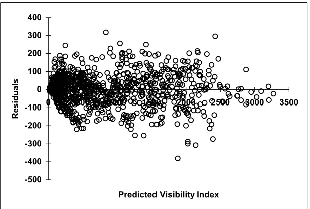
The residuals vs. the predicted absolute visibility indices plot (Figure 7) shows that the residuals are uniform and not extreme. Again note the magnitude of the residuals would make it difficult to estimate the Absolute visibility indices based on although a strong linear regression. This leads to the preliminary conclusion that though we have a very good global correlation with the Absolute visibility indices, i.e., an overall similarity, but an estimation of the Absolute visibility indices is theoretically implausible. In fact, it can be easily argued that it is impossible to pre-estimate the Absolute visibility index of a point. The reason is that it is theoretically not possible to model the LOS from a point, based on the properties of a point itself but can only be derived by actually drawing the LOS across the space. Therefore, the visibility index and viewshed are examples of the global properties of a point in contrast to the focal properties (e.g. elevation, slope etc.).
In the Method 2 for uncertainty estimation, we first generated 16 sets of 414 (the unique number of viewsheds based on Estimated visibility indices) spatially distributed random points. We then calculated the correlation coefficient between the Absolute- and Estimated- visibility indices for each of these sets of random points. The correlation coefficients are almost uniform averaging at 0.988540, with the exception of one case (0.990112), and an insignificant standard deviation of 0.001 (Figure 6b). The low standard deviation supports our earlier conclusion that our optimisation approach has reproduced the global pattern of the absolute visibility. However, dissimilarity with the Method 1 based correlation coefficient suggests that significant local variations would still exist.
In both cases, the Estimated visibility indices based on our simple approach have a much higher correlation coefficient than reported by Franklin et al. (1994) using his sophisticated algorithmic heuristics.
3.3 Significance of the Fundamental Topographic Features
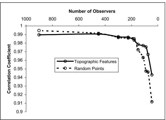
correlation between the Absolute- and Estimated- visibility indices is dependent upon both the spatial distribution and the topographical significance of the reduced number of observers but at low observer numbers, the topographical significance is a more useful basis. Thus, one could reduce the number of the topographic features for the visibility computation for large terrains with large number of topographic features, without the fear of losing any significant visibility information.
We believe that the divide between the topographic feature observers- and random observers- curves is likely to vary according to the characteristics of the each terrain, particularly large terrains will show a relatively wider separation between the curves than smaller terrains.
An interesting aspect of the Figure 8 is the overlap of the topographic feature observer- and random observer- correlation coefficient curves. It may indicate that in each terrain, there are observer densities at which both the topographic feature observers and random observers could provide an equal level of spatial optimisation. If this is proven, then it could be used as an indicator for the number of random observers selected to solve the time consuming minimum number of watchtowers problem (Lee, 1991). In hindsight, this overlap can also be an indicator for the optimal number of random points required in the method 2 for uncertainty estimation (see §2.1).
3.4 Optimisation of computation time
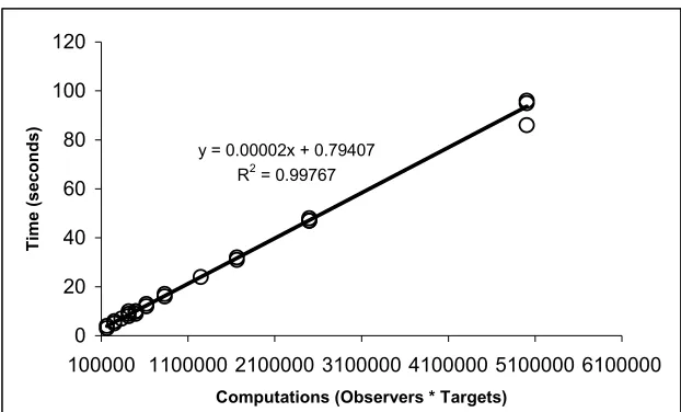
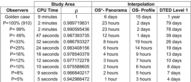
Figure 9 shows the relation between the CPU time usage vs. the various magnitudes of visibility computations performed in the work. Computations here represent the product of o*t. The plot expectedly shows a linear increase in the CPU time with an increase in the computations. If we assume that the DEM has a topographic feature density equal to the one in our study area, then the Table 1 shows the estimated time for the visibility computation for some popular DEM formats. As can be seen clearly the time saved is significant. However, the CPU time usage could be optimised even more by combining the current approach with the Reduced Targets Strategy such as done by Franklin et al. (1994).
3.5 Generalisation of the visibility pattern
4. Conclusion
In this work, we have shown that the use of the fundamental topographic features as observers (viewpoints), as part of the Reduced Observers Strategy, can be used to significantly decrease the visibility computation time without any significant visibility information loss. The reduced sampling of the observers in the terrain, however, introduces an uncertainty in the visibility indices. Based on our investigation, the residuals between the Absolute- and the Estimated- visibility indices are found to be uniform and random but significantly large that limits our ability to model Absolute visibility indices accurately.
The current work has found a number of interesting questions, which would be investigated in future works:
- The combination of the Reduced Observers Strategy and Reduced Targets Strategy will be investigated for the visibility computations on very large DEMs.
- The effect of the feature extraction scale on the visibility pattern will be investigated.
- The assumption that at certain observer densities, both a topographic features observers and random observers would produce similar quality of visibility estimation i.e., similar correlation coefficients between the Absolute- and the Estimated- visibility indices, will be validated. The relevance of this experiment for optimising accessibility analysis will be tested.
- The correlation coefficient provides only a global pattern matching but the visibility is a directional property. We will explore ways in which we could estimate the visual integrity in our optimised approach.
Acknowledgements
References
Crocetta, L., G. Gallo, and S. Spinello, 1998. Visibility in digital terrain maps: A fuzzy approach, Proceedings of the 14th Spring Conference on Computer Graphics, 23rd – 25th April, Budmerice, Slovakia, pp. 257-266.
De Floriani, L., and P. Magillo, 1994. Visibility algorithms on triangulated terrain models, International Journal of Geographical Information Systems, 8(1): 13–41.
De Floriani, L., P.K. Marzano, and E. Puppo, 1994. Line-of-sight communication on terrain models, International Journal of Geographical Information Systems, 8(4): 329-342.
Evans, I.S., 1979. An integrated system of terrain analysis and slope mapping, Final Report on Grant DA-ERO-591-73-G0040, University of Durham, Durham, UK.
Fisher, P.F., 1991. First experiments in viewshed uncertainty-the accuracy of the viewshed area, Photogrammetric Engineering and Remote Sensing, 57(10): 1321–1327.
Fisher, P.F., 1992. First experiments in viewshed uncertainty: simulating the fuzzy viewshed, Photogrammetric Engineering and Remote Sensing, 58(3): 345-352.
Fisher, P.F., 1993. Algorithm and implementation uncertainty in viewshed analysis, International Journal of Geographical Information Systems, 7(4): 331-347.
Franklin, W.M., C.K. Ray, and S. Mehta, 1994. Geometric algorithms for siting of air defense missile batteries, Technical Report, Contract No. DAAL03-86-D-0001, Battelle, Columbus Division, Columbus, Ohio, 116 p.
Franklin, W.M., 2000. Approximating visibility, Proceedings of the 1st International Conference on
Gibson, C., E. Ostrom, and T-K. Ahn, 1998. Scaling issues in the social sciences, http://www.uni-bonn.de/ihdp/WorkingPaper01/WP01.htm.
Greysukh, V.L., 1967. The possibility of studying landforms by means of digital computers, Soviet Geographer, 137-149.
Jenson, S.K., and J.O. Domingue, 1988. Extracting topographic structure from digital elevation data for geographic information systems analysis, Photogrammetric Engineering and Remote Sensing, 54(11): 1593-1600.
Jenks, G.F., 1963. Generalization in statistical mapping, Annals of the Association of American Geographers, 53: 15- 26.
Jennes, J., 2001, Random Point Generator Extension v.1.1 for ArcView, http://jennessent.com/arcview/random_points.htm.
Kim, Y-H., and K. Clarke, 2001. Exploring optimal visibility site selection using spatial optimisation techniques, Proceedings of GISRUK 2001, 18th – 20th April, University of Glamorgan,
Wales, pp. 141-146.
Lee, J., 1991. Analyses of visibility sites on topographic surfaces, International Journal of Geographical Information Systems, 5(3): 413-429.
Lee, J., 1992. Visibility dominance and topographical features on digital elevation models, Proceedings of the 5th International Symposium on Spatial Data Handling, Vancouver, Canada, pp.
622 – 631.
Lindeberg, T., 1994. Scale-space theory in computer vision, Kluwer Academic Press, Dordrecht, 423 p.
O’Sullivan, D., and A. Turner, 2001. Visibility graphs and landscape visibility analysis, International Journal of Geographical Information Systems, 15(3): 221-237.
Peucker, T. K., and D. H. Douglas, 1975. Detection of surface-specific points by local parallel processing of discrete terrain elevation data, Computer Graphics Image Processing, 4: 375-387.
Quattrochi, D.A., and M.F. Goodchild, 1996. Scale in Remote Sensing and GIS, Lewis Publishers, Boca Raton, Florida, 406 p.
Takahashi, S., T. Ikeda, Y. Shinagawa, T.L., Kunii, and M. Ueda, 1995. Algorithms for extracting correct critical points and constructing topological graphs from discrete geographical elevation data, The International Journal of the Eurographics Association, 14 (3): C-181- C-192.
Teng, A., D. Mount, E. Puppo, and L.S. Davis, 1997. Parallelizing an algorithm for visibility on polyhedral terrain, International Journal of Computational Geometry and Applications, 7(1&2): 75-84.
Wang, J., K. White, and G. Robinson, 1999. Estimating surface net solar radiation by use of Landsat-5 TM and digital elevation models, International Journal of Remote Sensing, 21(1): 31-43.
Wang, J., J. Robinson, and K. White, 2000. Generating viewsheds without using sightlines, Photogrammetric Engineering and Remote Sensing, 66(1): 87-90.
Ware, J.A., D.B. Kidner, P.J. Rallings, 1998. Parallel distributed viewshed analysis, Proceedings of the 6th international symposium on Advances in Geographic Information Systems, Washington DC, USA, pp 151-156.
Weibel, R. and G. Dutton, 1999. Generalising spatial data and dealing with multiple
Figure 2. Digital Elevation Model of the study area, in the SE Cairngorm Mountains, Scotland. Visualisation is based on the Natural Breaks Classification (Jenks, 1963) and Vertical exaggeration = 1.4.
803-901 718-802 649-718 583-648 505-582 395-504 902-1054 N
N
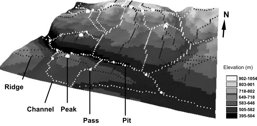
Figure 4. Fundamental topographic features of the study area draped over the DEM. The ridges originate at the peaks, the ridges and the channels meet at the passes, and the channels terminate at the pits. DEM visualisation is based on the Natural Breaks Classification (Jenks, 1963) and Vertical exaggeration = 1.4.
Peak
Pass Pit
Channel
Ridge 803-901
718-802 649-718 583-648 505-582 395-504 902-1054
Cor re lati o n Co eff ic ient 0. 990112 Best C ase 0. 989692 0. 989579 0. 989555 0. 989304 0. 989008 0. 988960 0. 988614 0. 988456 0. 988091 0. 988090 0. 987982 0. 987876 0. 987474 0. 987372 0. 986475 Worst Ca se
y = 0.1483x
+ 1.79
94
R
2 = 0.984
6 0 100 200 300 400 500 600 0 500 1000 1500 2000 2500 3000 3500 A b so lu te V is b ility In d ex Es timated Visibility Index
ρx,y = 0.9922 63 n = 910 Figure 6 . As sess
ment of u
ncertainty
by (a)
co
m
paris
on between t
he Absolute-
and the Esti
mated- visibil
ity
indices of the fundam
ent
al topographic features,
and (b) comparison between the
Absolute-and the
Esti
m
ated- vi
sibilit
y indices correlation coeffici
ents o
f 16 different
sets of random
points.
(a)
-500 -400 -300 -200 -100 0 100 200 300 400
0 500 1000 1500 2000 2500 3000 3500
Predicted Visibility Index
Residuals
Figure 7. Distribution of the residuals in the regression (Figure 6a)
between the Absolute- and Estimated- visibility indices of the
0.9 0.91 0.92 0.93 0.94 0.95 0.96 0.97 0.98 0.99 1
0 200
400 600
800 1000
Number of Observers
Corre
la
tion Coe
ffic
ie
n
t
Topographic Features Random Points
Figure 8. Comparison between the Absolute- and the Estimated- visibility
indices correlation coefficients, for a decreasing number of topographic
y = 0.00002x + 0.79407
R2 = 0.99767
0 20 40 60 80 100 120
100000 1100000 2100000 3100000 4100000 5100000 6100000
Computations (Observers * Targets)
Time (seconds)
Figure 9. Linear increase in the visibility computation time with varying
Study Area Interpolation
Observers CPU Time ρ OS*- Panorama OS- Profile DTED Level 1
Golden case 9 minutes 1 6 days 15 days 1 year
P=100% (910) 2 minutes 0.989719831 23 hours 2 days 79 days
P= 99% 2 minutes 0.990595436 23 hours 2 days 78 days
P= 49% 47 seconds 0.987393735 12 hours 1 days 39 days
P=33% 32 seconds 0.986793327 8 hours 19 hours 26 days
P=25% 24 seconds 0.983408156 6 hours 14 hours 19 days
P=16% 16 seconds 0.978540379 4 hours 9 hours 13 days
P=12% 12 seconds 0.977172278 3 hours 7 hours 10 days
P=10% 10 seconds 0.975588605 2 hours 6 hours 8 days
P=8% 9 seconds 0.966840217 2 hours 5 hours 7 days
P=5% 5 seconds 0.942986472 1 hour 3 hours 4 days
Table 1. CPU usage times for the visibility computation in the study area and the
interpolation of the experiment’s time-observer density combinations to some
standard DEM formats. * OS – Ordnance Survey, UK, Landform data. In all cases,
the viewers can see to the infinity. All the durations have been rounded off to the