POUR L'OBTENTION DU GRADE DE DOCTEUR ÈS SCIENCES
acceptée sur proposition du jury: Dr M. Mattavelli, président du jury Prof. J.-Ph. Thiran, directeur de thèse
Prof. G. Potamianos, rapporteur Prof. T. Schultz, rapporteuse Dr J.-M. Odobez, rapporteur
Visual speech recognition: from traditional to deep
learning frameworks
THÈSE NO 8799 (2018)
ÉCOLE POLYTECHNIQUE FÉDÉRALE DE LAUSANNE
PRÉSENTÉE LE 31 AOÛT 2018
À LA FACULTÉ DES SCIENCES ET TECHNIQUES DE L'INGÉNIEUR LABORATOIRE DE TRAITEMENT DES SIGNAUX 5 PROGRAMME DOCTORAL EN GÉNIE ÉLECTRIQUE
PAR
Acknowledgements
This work would not have been possible without the support of many others. Therefore, I would like to acknowledge their contributions at this point.
First of all, I would like to thank my thesis director Prof. Jean-Philippe Thiran. Thank you for always being supportive and encouraging, especially in moments where no solution seemed to be in sight. In the last two years I was also very lucky to work together with Prof. Hazım Kemal Ekenel. Thank you for all the detailed discussions and the scientific supervision. I would also like to thank the jury members of my thesis oral examination, Dr Marco Mattavelli, Prof. Gerasimos Potamianos, Prof. Tanja Schultz and Dr Jean-Marc Odobez, for their detailed feedback and insightful comments.
Along this journey I have worked with many people: Thank you to Estelle Chin and Olivier Payot for the collaboration with PSA in the beginning. Thank you also to Dr Mathew Magimai-Doss for several discussions on speech recognition when I was diving deeper into these topics.
I would also like to thank all the current and former members of LTS5, for common lunches, matches of ‘baby-foot’ or other activities: Alessandra, Alessandro, Alia, Alice, Anıl, Anna, Audrey, Behzad, Carlos, Christina, Christophe E., Christophe P., Damien, David, Didrik, Dimitri, Elda, Elena, Frank, Gabriel C., Gabriel G., Gaëtan, Hua, Jelena, Jonathan, Marco, Mário, Mina, Ming, Muhamed, Murat, Rafael, Ricardo, Saeed, Saleh, Tom, Vijay and others. Since we share the corridor with the other signal processing labs, I was also happy to meet Anne-Flore, Eda, Hamed, Raphaël, Sasan, Sibylle and many others there and spend time with them on and off campus. I am also very glad I could work within the ‘Face group’, a sub-group of LTS5: thank you Anıl, Behzad, Damien, Hazım, Hua, Gabriel, Murat, Saeed, Saleh. Thank you also to my office mates over the years: Gabriel, Alessandro, Anna, Tim and Damien.
Without the organisational skills of Rosie, and lately Anne, the labs would surely have trouble finishing all the administrative work on time. Thank you for all your help and nice chats.
Since a PhD is not only work, I would also like to thank all those who made lunches, dinners and trips in and outside Lausanne more fun: Audrey, Carlos, Deniz, Didrik, Elena, Gabriel, Hyunjin, Irene, Marili, Mário, Maya, Mina, Murat, Olivia, Ricardo, Sasan, Tom and Vijay. Thank you also to all my friends outside EPFL who reminded me that there is indeed a world out there: Akshara, Alexandra F., Alexandra P., Amandine, Ana, Angela, Bity, Eva, Laura, Linn, Lisa, Kathi, Kerstin, Khushboo, Simone, Sophie
and Vivienne.
A heartfelt thank you to Vijay, who accompanied me along this journey and lent a helping hand where necessary and skipped along the path with me during happy moments. Finally, I would like to thank my family for their continuous support and words of encouragement. Thank you in particular to my parents who showed me never to give up.
Abstract
Speech is the most natural means of communication for humans. Therefore, since the beginning of computers it has been a goal to interact with machines via speech. While there have been gradual improvements in this field over the decades, and with recent drastic progress more and more commercial software is available that allow voice commands, there are still many ways in which it can be improved.
One way to do this is with visual speech information, more specifically, the visible articulations of the mouth. Based on the information contained in these articulations, visual speech recognition (VSR) transcribes an utterance from a video sequence. It thus helps extend speech recognition from audio-only to other scenarios such as silent or whispered speech (e.g. in cybersecurity), mouthings in sign language, as an additional modality in noisy audio scenarios for audio-visual automatic speech recognition, to better understand speech production and disorders, or by itself for human machine interaction and as a transcription method.
In this thesis, we present and compare different ways to build systems for VSR: We start with the traditional hidden Markov models that have been used in the field for decades, especially in combination with handcrafted features. These are compared to models taking into account recent developments in the fields of computer vision and speech recognition through deep learning. While their superior performance is confirmed, certain limitations with respect to computing power for these systems are also discussed. This thesis also addresses multi-view processing and fusion, which is an important topic for many current applications. This is due to the fact that a single camera view often cannot provide enough flexibility with speakers moving in front of the camera. Technology companies are willing to integrate more cameras into their products, such as cars and mobile devices, due to lower hardware cost for both cameras and processing units, as well as the availability of higher processing power and high performance algorithms. Multi-camera and multi-view solutions are thus becoming more common, which means that algorithms can benefit from taking these into account. In this work we propose several methods of fusing the views of multiple cameras to improve the overall results. We can show that both, relying on deep learning-based approaches for feature extraction and sequence modelling, as well as taking into account the complementary information contained in several views, improves performance considerably. To further improve the results, it would be necessary to move from data recorded in a lab environment, to multi-view data in realistic scenarios. Furthermore, the findings and models could be
transferred to other domains such as audio-visual speech recognition or the study of speech production and disorders.
Key words: visual speech recognition; automatic lip-reading; multi-view processing; GMM-HMM; deep learning
Résumé
La parole est la forme de communication la plus naturelle des humains. C’est la raison pour laquelle, depuis le début des ordinateurs, on a cherché à interagir avec les machines à travers la parole. Bien qu’il y ait eu des améliorations graduelles dans ce domaine pendant des décennies, et qu’il existe de plus en plus de programmes commerciaux qui permettent des commandes vocales, bon nombre de points doivent encore être améliorés. Pour ce faire, une méthode utilise les informations de la parole visuelle, ou plus particulièrement, les articulations visibles de la bouche.
Basée sur les informations contenues dans ces articulations, la reconnaissance de la parole visuelle transcrit un énoncé depuis une séquence vidéo. Ainsi, elle permet d’étendre la reconnaissance de la parole de l’audio uniquement à d’autres scénarios, tels que : la parole silencieuse ou chuchotée utile pour la sécurité informatique, les « mouthings » (articula-tions des lèvres) de la langue des signes, une modalité de plus dans les scénarios d’audio bruité pour la reconnaissance de la parole audio-visuelle, une meilleure compréhension de la production de la parole ou des troubles du langage, l’interaction homme-machine ou une méthode de transcription.
Dans cette thèse, nous présentons et comparons des manières différentes de développer des systèmes de reconnaissance de la parole visuelle. Nous commençons par étudier les modèles de Markov cachés traditionnels, utilisés dans ce domaine pendant des décennies, en particulier en combinaison avec des caractéristiques choisies manuellement. Puis, nous comparons ces systèmes à des modèles qui prennent en compte les développements récents, par l’apprentissage profond, dans les domaines de la vision par l’ordinateur et de la reconnaissance de la parole. Même si leur performance supérieure est confirmée, il est important de souligner certaines limites concernant leur besoin de puissance de calcul. Cette thèse développe aussi le traitement et la fusion de plusieurs angles de vues, ce qui est un sujet important pour beaucoup d’applications récentes. Cela est dû au fait qu’une seule caméra ne peut pas donner assez de flexibilité au locuteur qui bouge devant celle-ci. Les entreprises de technologie sont prêtes à intégrer plusieurs caméras dans leurs appareils, comme les voitures ou les appareils portables, suite à la baisse des prix des caméras et des processeurs, aux puissances de calcul plus élevées et aux algorithmes plus performants. Des solutions multi-caméra et multi-vue deviennent ainsi plus communes, ce que requièrent les algorithmes pour les prendre en compte. Dans ce travail, nous proposons plusieurs méthodes pour la fusion de vues de plusieurs caméras, afin d’améliorer les résultats finaux.
Nous pouvons constater que les deux approches : se baser sur l’apprentissage profond pour l’extraction de caractéristiques et la modélisation de séquences, ainsi que prendre en compte l’information complémentaire contenue dans plusieurs vues, améliore fortement la performance. Afin d’améliorer les résultats, il serait nécessaire de changer les données enregistrées dans un environnement de laboratoire, en données de plusieurs vues dans les scénarios réalistes. En outre, les résultats et les modèles pourraient être transposés à quelques autres domaines comme la reconnaissance de la parole audio-visuelle ou l’investigation de la production de la parole et des troubles du langage.
Mots clefs : reconnaissance de la parole visuelle ; lecture labiale automatique ; traitement de plusieurs vues ; MMG-MMC ; apprentissage profond
Zusammenfassung
Sprache ist die natürlichste Form der menschlichen Kommunikation. Daher existiert seit der Erfindung des Computers das Ziel, mit den Maschinen über Sprache zu interagieren. Auch wenn auf diesem Gebiet in den letzten Jahrzehnten kontinuierliche Fortschritte erreicht wurden und immer mehr Computerprogramme Sprachkommandos ermöglichen, gibt es weiterhin viele Verbesserungsmöglichkeiten.
Eine Möglichkeit der Optimierung besteht in den visuellen Sprachinformationen, präziser, in den sichtbaren Mundbewegungen. Gestützt auf die darin enthaltenen Informationen transkribiert die visuelle Spracherkennung die Äußerung einer Videosequenz. Dies erlaubt, die Spracherkennung von reinem Audio auf andere Szenarien auszuweiten, wie beispiels-weise auf lautlose oder geflüsterte Sprache (z. B. in der Computersicherheit), „Mouthings“ (Lippenbewegungen) in der Gebärdensprache, als zusätzliche Modalität in geräuschvollen
Audioszenarien für audio-visuelle Spracherkennung, zum besseren Verständnis von Sprach-produktion und Sprechstörungen oder alleine für die Mensch-Computer-Interaktion und als Methode zur Transkription von Videos.
In dieser Doktorarbeit präsentieren und vergleichen wir verschiedene Methoden zur Ent-wicklung eines visuellen Spracherkennungssystems: Wir beginnen mit den traditionellen Hidden-Markov-Modellen, die in diesem Bereich jahrzehntelang eingesetzt waren, vor allem in Kombination mit handverlesenen Merkmalen. Diese werden mit Modellen vergli-chen, die die neuesten Entwicklungen auf dem Gebiet des maschinellen Sehens und der Spracherkennung durch das Deep Learning einbeziehen. Deren bessere Leistung wird be-stätigt, jedoch werden auch bestimmte Einschränkungen in Bezug auf die Rechenleistung für diese Systeme besprochen.
Diese Doktorarbeit behandelt auch die Verarbeitung mehrerer Kameraansichten und deren Fusion, die ein wichtiges Thema für viele aktuelle Anwendungen sind, weil eine einzige Kameraansicht nicht genügend Flexibilität bietet, wenn die Sprecher sich vor der Kamera bewegen. Technologieunternehmen integrieren inzwischen mehrere Kameras in ihre Produkte, wie Autos, mobile Geräte usw., da die Hardwarekosten sowohl für Kameras als auch für Prozessoren gesunken und gleichzeitig auch Rechenleistungen und die Performance der Algorithmen gestiegen sind. Multikamera- und Multiansicht-Lösungen verbreiten sich dadurch stärker, und daher sollten Algorithmen diese berücksichtigen. In dieser Arbeit stellen wir mehrere Methoden für die Fusion verschiedener Kameraansichten vor, um die Gesamtergebnisse zu verbessern.
Merkmalen und zur Modellierung von Sequenzen als auch die Nutzung von ergänzenden Informationen aus mehreren Kameraansichten die Leistung erheblich steigern. Um die Ergebnisse weiter zu optimieren, wäre es nötig, von Videoaufnahmen im Labor hin zu Multiansichts-Daten aus realistischen Szenarien zu wechseln. Außerdem sollten die Erkenntnisse und Modelle in anderen Bereichen wie der audio-visuellen Spracherkennung oder der Untersuchung von Sprachproduktion und Sprechstörungen angewandt werden. Stichwörter:visuelle Spracherkennung; automatisches Lippenlesen; Verarbeitung mehrerer Kameraansichten; GMM-HMM; Deep Learning („tiefgehendes Lernen“)
Contents
Acknowledgements iii
Abstract (English/Français/Deutsch) v
List of figures xiii
List of tables xv
List of acronyms xvii
Introduction 1
Motivation . . . 1
Thesis outline . . . 2
Contributions . . . 3
1 Background 5 1.1 Visual speech classes . . . 5
1.2 Video preprocessing: face tracking . . . 6
1.3 Traditional approaches . . . 9
1.3.1 Visual feature extraction . . . 9
1.3.2 Sequence modelling . . . 11
1.4 Combined approaches . . . 13
1.4.1 Visual feature extraction . . . 14
1.4.2 Sequence modelling . . . 16
1.5 Deep learning approaches . . . 17
1.5.1 Feature extraction . . . 17
1.5.2 Sequence modelling . . . 17
1.6 Performance metrics . . . 23
1.7 Multi-view visual speech recognition . . . 23
1.8 Databases . . . 25
1.8.1 TCD-TIMIT . . . 25
2 Traditional approach 31 2.1 Motivation . . . 31 2.2 Proposed method . . . 32 2.3 Performance analysis . . . 33 2.3.1 The datasets . . . 33 2.3.2 Experimental results . . . 33 2.4 Summary . . . 37 3 Combined approach 41 3.1 Motivation . . . 41 3.2 Proposed method . . . 42 3.3 Performance analysis . . . 44 3.3.1 The dataset . . . 44 3.3.2 Experimental results . . . 44 3.4 Summary . . . 47
4 Deep learning approach 51 4.1 Motivation . . . 51
4.2 Proposed method . . . 52
4.2.1 Feature extraction using convolutional neural networks . . . 52
4.2.2 Sequence modelling with recurrent neural networks . . . 55
4.2.3 Decoding with connectionist temporal classification . . . 57
4.3 Performance analysis . . . 57
4.3.1 The dataset . . . 58
4.3.2 Experimental results . . . 59
4.4 Summary . . . 70
5 Multi-view visual speech recognition 73 5.1 Motivation . . . 73 5.2 Proposed method . . . 74 5.3 Performance analysis . . . 75 5.3.1 The dataset . . . 75 5.3.2 Experimental results . . . 76 5.4 Summary . . . 83 Conclusion 85 Perspectives . . . 86 Bibliography 89 Curriculum vitae 99
List of figures
1.1 Flowchart of the visual speech recognition chain. . . 5
1.2 Face tracking examples using the SDM-based face tracker. . . 8
1.3 Sequence modelling with a GMM-HMM system. . . 13
1.4 Schematic of an MLP. . . 14
1.5 Schematic of the basic building blocks of a CNN. . . 16
1.6 Schematic of an LSTM cell. . . 19
1.7 Schematic of a GRU. . . 20
1.8 Schematic of a bidirectional RNN . . . 20
1.9 Examples from the TCD-TIMIT database. . . 26
1.10 Examples from the OuluVS2 database. . . 28
2.1 Flowchart of the GMM-HMM system used. . . 32
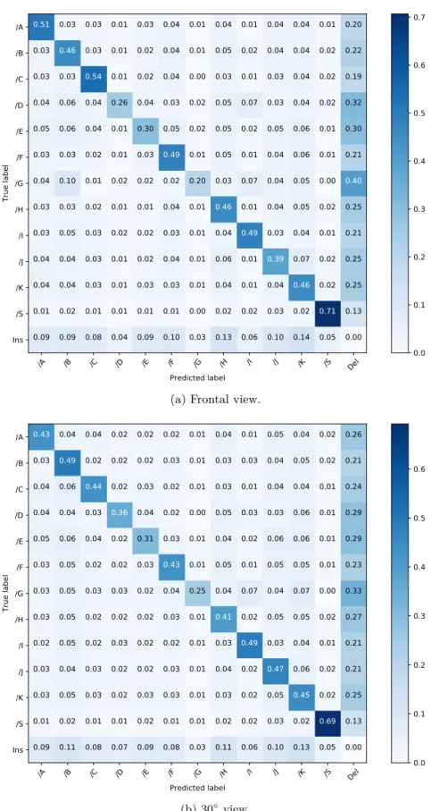
2.2 Phrase recognition results on OuluVS2 using a simple GMM-HMM model. 34 2.3 Viseme recognition results on TCD-TIMIT using a simple GMM-HMM model. . . 37
2.4 Confusion matrices of our simple GMM-HMM model for the frontal and 30◦ views. . . 38
3.1 The proposed tandem system with PCA network-LSTMs and GMM-HMMs for VSR. . . 43
3.2 The PCA network used in the first stage of the proposed tandem system. 44 3.3 Phrase recognition results on OuluVS2 using the proposed tandem system with cross-validation. . . 46
3.4 Phrase recognition results on OuluVS2 using the proposed tandem system on the test set. . . 47
4.1 Flowcharts of the different CNN architectures. . . 54
4.2 Flowchart of the RNN network integrated with the CNN. . . 56
4.3 Histogram of the visemes in the TCD-TIMIT database. . . 60
4.4 Evolution of loss during training. . . 61
4.5 Evolution of categorical accuracy during training. . . 61
4.6 Confusion matrices of the two best CNNs. . . 64
4.7 Confusion matrix of the best RNN. . . 66 4.8 Viseme recognition results on TCD-TIMIT using our CNN-RNN with CTC. 68
4.9 Confusion matrices of our CNN-RNN with CTC for the frontal and 30◦
views. . . 69 5.1 The proposed feature fusion multi-view tandem system with PCA
network-LSTMs and GMM-HMMs for VSR. . . 75 5.2 Multi-view phrase recognition results on OuluVS2 using feature fusion in
the proposed tandem system with cross-validation. . . 79 5.3 Multi-view phrase recognition results on OuluVS2 using feature fusion in
the proposed tandem system on the test set. . . 80 5.4 Best multi-view phrase recognition results on OuluVS2 using the proposed
List of tables
1.1 Viseme mapping used in this work. . . 7
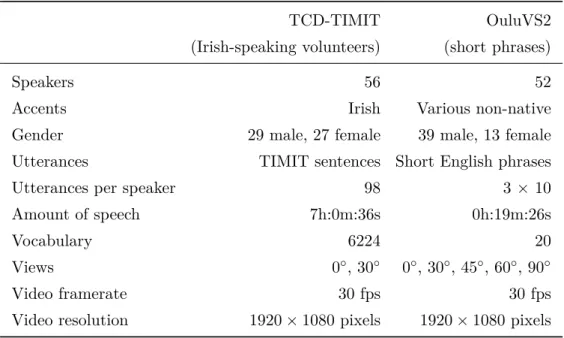
1.2 Overview over the TCD-TIMT and OuluVS2 databases. . . 26
1.3 Example sentences from the TIMIT dataset. . . 27
1.4 Training and test splits for the TCD-TIMIT dataset. . . 27
1.5 List of short phrases from the OuluVS2 dataset. . . 28
1.6 Training and test splits for the OuluVS2 dataset. . . 29
2.1 Phrase recognition results on OuluVS2 using a simple GMM-HMM model with silence label. . . 35
2.2 Phrase recognition results on OuluVS2 using a simple GMM-HMM model without silence label. . . 36
2.3 Viseme recognition results on TCD-TIMIT using a simple GMM-HMM model. . . 40
3.1 Baseline sentence recognition results on OuluVS2 by the authors of the database. . . 45
3.2 Phrase recognition results on OuluVS2 using the proposed tandem system on the test set. . . 48
3.3 Frame recognition results on OuluVS2 using the LSTM output. . . 49
4.1 Comparison of model sizes for the different CNN architectures. . . 53
4.2 Comparison of model sizes for the different RNN architectures. . . 55
4.3 Framewise viseme accuracy validation results on the frontal view of TCD-TIMIT using the different CNN architectures. . . 62
4.4 Framewise viseme accuracy test results on the frontal view of TCD-TIMIT using the different CNN architectures. . . 62
4.5 Framewise viseme accuracy validation results on the frontal view of TCD-TIMIT using the different RNN architectures. . . 65
4.6 Framewise viseme accuracy test results on the frontal view of TCD-TIMIT using the different RNN architectures. . . 65
4.7 Viseme recognition test accuracy on the frontal and 30◦ views of TCD-TIMIT using different RNN architectures with CTC. . . 66 4.8 Viseme recognition results on TCD-TIMIT using our CNN-RNN with CTC. 71
5.1 Multi-view phrase recognition results on OuluVS2 using feature fusion in the proposed tandem system on the test set. . . 77 5.2 Optimal weights for the proposed multi-view tandem system. . . 78 5.3 Best multi-view phrase recognition results on OuluVS2 using the proposed
List of acronyms
AAM active appearance model
ANN artificial neural network ASR automatic speech recognition
AVASR audio-visual automatic speech recognition
BGRU bidirectional GRU
BLSTM bidirectional LSTM
BRNN bidirectional RNN
CNN convolutional neural network
CTC connectionist temporal classification DCT discrete cosine transform
DNN deep neural network
DWT discrete wavelet transform
GMM Gaussian mixture model
GPU graphics processing unit
GRU gated recurrent unit
HCI human computer interaction
HiLDA hierarchical LDA
HMM hidden Markov model
LBP-TOP local binary patterns from three orthogonal planes LDA linear discriminant analysis
LGO local gradient orientation
LSTM long short-term memory
MLLT maximum-likelihood linear transform
MLP multilayer perceptron
PCA principle component analysis
PDM point density model
RBM restricted Boltzmann machine
RNN recurrent neural network
ROI region of interest
SDM supervised descent method
SIFT scale-invariant feature transform VSR visual speech recognition
Introduction
Speech is an important means of human communication, and at its level of complexity it is often considered to be one of the distinctive characteristics between humans and other animals. Speech is also one of the most natural ways of communication for humans, and thus has long been dreamt up in human computer interaction (HCI) to facilitate the interaction between humans and machines and to make it more natural. With advances in signal processing and increasing computational power, algorithms were developed that could transcribe an audio signal to a sequence of phonetically distinct units. However, only with further developments in both technology and algorithms, could the machines recognise a larger vocabulary and eventually react to the commands. Still, the interaction is often frustrating when there are misunderstandings, which can happen particularly in noisy situations. Or it might be undesirable to have your neighbour listen in on your commands, e.g. when spelling out your password. Furthermore, hearing impaired people communicate via sign language, rather than using spoken words. For all these, another branch of speech recognition, using the visible articulations of the mouth, has developed: visual speech recognition (VSR) or automatic lip-reading.
There are many applications to this field, including the examples mentioned above, such as support for the audio in noisy situations through audio-visual automatic speech recognition [Potamianos et al., 2004], silent or whispered speech, e.g. for pronouncing passwords in cybersecurity [Denby et al., 2010, Hassanat, 2014, Petridis et al., 2018], for the mouthings in sign language recognition [Schmidt and Koller, 2013], as well as understanding speech production better [Badin et al., 2002] or for direct HCI.
Motivation
The interest in visual speech recognition is motivated by the way humans work when confronted with a listening task or conversation in a very noisy environment. In situations such as a noisy restaurant humans usually resort to lip reading to improve their under-standing. Humans make use of the additional information to distinguish different sounds. When simultaneously listening and lip reading, a sound can even be confused if the wrong mouth movement is shown: this is the McGurk effect [McGurk and MacDonald, 1976].
We can exploit this extra information in audio-based automatic speech recognition as well by combining audio and video modalities.
In this thesis the focus is on pure VSR which can then be used as a starting point for other research problems like the ones mentioned above. The aim of this work is to show the improvements that can be obtained starting from the traditional hand-crafted feature and GMM-HMM systems, via combined approaches using neural networks to extract features while still maintaining the GMM-HMM system, all the way to fully deep learning-based methods with CNNs and RNNs. It also shows the limitations of certain methods, considering the data size and using only a single computer and graphics processing unit (GPU).
A remaining constraint of VSR is the inability to deal with videos coming from different view angles. This is a major problem for applying these algorithms in real-life situations, since in most cases the speaker is free to move his head or even the entire body. For these reasons and due to the availability of cheaper equipment, it is becoming more popular nowadays to increase the number of cameras on a device or in a certain environment. For example, it is becoming more common to integrate at least two cameras into a car to monitor the driver. Here the question of how to treat these different video streams and how to combine their information comes into play. This topic is treated in this thesis, albeit for static views. The choice of databases analysed is also determined by this factor, whether it provides several simultaneously recorded views.
Thesis outline
The thesis is structured in the following way:
• To begin, Chapter 1: Background provides an overview of the methods needed and used in VSR. This ranges from the definition of the speech classes, over the face tracking needed to preprocess the videos, to approaches used for visual feature extraction and sequence modelling. In the latter, three types of approaches are elaborated: the traditional approaches, the combined, and the most recent deep learning-based methods. This is followed by an overview of the performance metrics used in this thesis. Finally, a short introduction to multi-view visual speech recognition and the databases explored in this work are given.
• Chapter 2: Traditional approach outlines the setup and presents some baseline results performed with handcrafted features (DCT coefficients) with standard GMM-HMM systems.
• InChapter 3: Combined approacha feature extraction system consisting of a PCA network followed by an LSTM is presented. In a tandem system these features are
Contributions then passed into a GMM-HMM which models the time evolution. It is shown that this network outperforms the traditional methods presented as a baseline.
• Following the advances in deep learning, Chapter 4: Deep learning approach provides a systematic step-by-step approach to developing a deep learning system. It is shown that this method outperforms the previous approaches.
• Taking into account the views from different camera angles,Chapter 5: Multi-view visual speech recognition uses the tandem approach to show that the combination can improve the results by integrating the complementary information.
• Finally, Conclusion summarises the results presented in this thesis and provides an outlook on future research.
Contributions
The main contributions of this thesis are summarised below:
• Provide an overview over the different approaches from the traditional to deep learning methods.
• Design a novel tandem system composed of PCA networks with LSTM and a GMM-HMM suitable for small databases [Zimmermann et al., 2017a].
• Propose a systematic approach to developing a deep learning system for continuous sequence-to-sequence visual speech recognition.
• Implement a new method to weight the contributions of different views for multi-view visual speech recognition with a tandem system [Zimmermann et al., 2017b].
1
Background
This chapter provides background information on visual speech recognition (VSR) and the methods used in the field, coming from both the speech recognition and computer vision domains. First the visual speech classes used in this thesis are elaborated. This is followed by an overview of face tracking, needed to find the relevant regions of the face. The subsequent sections present various approaches to VSR: from the traditional approaches with handcrafted features and GMM-HMMs via combined approaches to end-to-end deep learning models. For each approach the processing steps for VSR shown in Figure 1.1 are elaborated: first the features are extracted from the input video frames and then the feature sequence is modelled in time to obtain the sequence of output labels. Next, the performance metrics applied in this work are presented and an overview of multi-view lip reading is given. Finally, existing (audio-)visual speech databases are discussed and those used in this thesis are described in more detail.
1.1
Visual speech classes
One of the first decisions to take when building a speech recognition system involving video is the choice of classes to distinguish different sounds or rather articulations for VSR. In audio-based speech recognition the classes are usually phonemes, defined as the smallest distinctive linguistic unit, or phones, the unit of speech sound independent of the language [Coxhead, 2006]. However, in video-based speech recognition several
Parts of this chapter have been published by Zimmermann et al. [2017a,b].
Input video Feature extraction Sequence modelling Output label sequence
phonemes look the same or similar, so they are usually grouped into visually distinct units called visemes [Cappelletta and Harte, 2012]. Several many-to-one mappings exist from phonemes to visemes. These are usually made up of around 8 to 17 different viseme classes [Coxhead, 2006, Turkmani, 2007, Souviraà-Labastie and Bimbot, 2013]. Even though some research has suggested that visemes provide a sub-optimal classification of speech data [Bear et al., 2014, Yu et al., 2011], some type of visemes or even phonemes are still generally preferred, since they easily relate to phonemes in audio recognition and are thus easy to understand for humans and easily fused in audio-visual automatic speech recognition (AVASR).
In this work we do VSR for English and use the same viseme set as the one used by [Harte and Gillen, 2015], initially proposed in [Jeffers and Barley, 1971]. The choice is based on two factors: first, this mapping has been shown to be reliable [Cappelletta and Harte, 2012]. Secondly, it is used in the baseline results for the database TCD-TIMIT proposed in [Harte and Gillen, 2015], which will be used for part of this work. Using the same viseme set allows better comparisons between different approaches.
However, other types of classes have also been used in the literature. Some recent studies use graphemes rather than phonemes or visemes, which are the different letters, numbers, characters and punctuation marks that appear in a written sentence [Chung and Zisserman, 2017]. For smaller datasets sometimes whole words are used as the smallest unit [Wand et al., 2016]. Finally, some research only tries to distinguish between a set of predefined sentences [Lee et al., 2017, Saitoh et al., 2017].
In contrast to these, in this thesis generally visemes are used as smallest units and sequence-to-sequence decoding is performed, rather than classifying whole utterances. On the smaller one of the two datasets treated in this work, these viseme sequences are then regrouped to word-level models which are then decoded to a sequence of words. For the larger dataset the smallest unit in the sequence decoding are visemes.
1.2
Video preprocessing: face tracking
When treating facial video, it is important to focus on the particular region of interest (ROI) on the face. For VSR, this means extracting the areas which are active during articulation and which thus provide the largest amount of information about the utterance: the mouth, in particular the lips, and possibly other regions such as the cheeks and jaws. To find these ROIs, newer studies generally apply face trackers that detect the face and find specific landmarks on the face and track these over consecutive frames (an example is shown in Figure 1.2), while older works rely on manually labelling or on markers such as lipstick. The most common choice nowadays for detecting the face is still the Viola-Jones face detector, using features similar to the Haar basis functions [Viola and Jones, 2001].
1.2. Video preprocessing: face tracking Table 1.1 – Viseme mapping for English by Jeffers and Barley [1971] as presented by Harte and Gillen [2015] used in this work.
Viseme TIMIT phonemes Description
/A /f/, /v/ Lip to teeth
/B /er/, /ow/, /r/, /q/, /w/, Lips puckered
/uh/, /uw/, /axr/, /ux/
/C /b/, /p/, /m/, /em/ Lips together
/D /aw/ Lips relaxed-moderate opening
to Lips puckered-narrow
/E /dh/, /th/ Tongue between teeth
/F /ch/, /jh/, /sh/, /zh/ Lips forward
/G /oy/, /ao/ Lips rounded
/H /s/, /z/ Teeth approximated
/I /aa/, /ae/, /ah/, /ay/, /ey/, /ih/, /iy/, /y/, Lips relaxed narrow opening /eh/, /ih/, /iy/, /y/, /eh/, ax-h/, /ax/, /ix/
/J /d/, /l/, /n/, /t/, /el/, /nx/, /en/, /dx/ Tongue up or down
/K /g/, /k/, /ng/, /eng/ Tongue back
/S /sil/, /pcl/, /tcl/, /kcl/, /bcl/, /dcl/, Silence
/gcl/, /h#/, /#h/, /pau/, /epi/
For subsequent tracking, various types of face trackers exist. One of the most commonly used trackers in VSR is the active appearance model (AAM) [Cootes et al., 2001], since its parameters are sometimes directly used as features.
AAMs model both facial shape and appearance. The shape of the AAM is described by the sequence of (x, y) coordinates of the landmark locations in the model: s =
(x1, y1, . . . , xn, yn)
This shape is parametrised with a principle component analysis (PCA), so that it can be represented as a sum of the mean shape s0 and its eigenvectors si multiplied by the
shape parameters pi [Lan et al., 2010]:
s=s0+
m
X
i=1
(a) Frontal view, mouth open. (b) Side view, mouth open.
(c) Frontal view, mouth closed. (d) Side view, mouth closed.
Figure 1.2 – Face tracking and mouth cropping examples with the facial landmarks indicated on frames from the TCD-TIMIT database using the SDM-based face tracker. Here the m largest eigenvectors are kept, where
p=sT(s−s
0). (1.2)
Similarly, the appearanceAwithin this region can be described as a linear combination of a decomposition by PCA into mean appearance and eigenvectors with the corresponding appearance parameters qi: A=A0+ l X i=1 qiAi. (1.3)
This is applied to shape-normalised and reshaped images and thellargest eigenvectors
are stored. Again,
q=AT(A−A
0). (1.4)
However, more recent face trackers, like the regression-based one using the supervised descent method (SDM) [Xiong and De la Torre, 2013] for fitting, show better performance results for facial landmark tracking [Cuendet, 2017]. This fitting method has been developed to minimise non-linear least squares functions. Unlike the parametrised AAM described above, regression-based face trackers do not use a shape or appearance model,
1.3. Traditional approaches but learn the vectorial regression function from the image directly on the landmark locations s = (x1, y1, . . . , xn, yn). This allows the tracker to more readily adapt to
asymmetric shapes or untrained gestures. The landmark locations are updated iteratively through a sequence of descent directions and rescaling factors (sk+1 =sk+∆s).
Finally, another difference from the AAM is the use of scale-invariant feature transform (SIFT) features around each landmark location in the SDM. The feature vector φ∗
contains the collected and ordered features of a particular shape s∗ in an image, and
is directly used to compute the necessary updates. Due to its better performance, an implementation of the SDM-based face tracker from our lab, with improvements from [Qu et al., 2015], is used where necessary in this work to crop the ROI.
1.3
Traditional approaches
This section describes the traditional approach to visual speech recognition, which comprises the extraction of texture-based or geometrical features and the consequent modelling of specific speech classes through hidden Markov models (HMMs) with Gaussian mixture models (GMMs). It is structured in the following way: first visual feature extraction techniques and then sequence modelling with a GMM-HMM system are discussed.
1.3.1 Visual feature extraction
After deciding on the type of class and obtaining the correct landmark locations, it is necessary to look into the different features used in visual speech recognition. They can be grouped into two approaches: appearance-based and shape-based features [Potamianos et al., 2004].
Appearance-based features exploit the pixel values in the ROI and apply a sort of transformation to these. Popular image transformations include the PCA, discrete cosine transform (DCT), discrete wavelet transform (DWT), linear discriminant analysis (LDA) and maximum-likelihood linear transform (MLLT) [Potamianos et al., 2004]. These can be applied at different stages of a feature extraction framework.
PCA, DCT and DWT are image transformation methods that compress the information in the ROI, while LDA improves classification by remapping the data to a different feature space where the discriminability is maximised; similarly, MLLT is a maximum likelihood data modelling technique. The latter two can be used not only on appearance-based features but also for post-processing of any kind of feature [Potamianos et al., 2004]. Shape-based features, on the other hand, extract information about the shape of the mouth. As summarised by Potamianos et al. [2004], various shape-related features have
been explored in the literature. This can be done for example with the help of active contour models, or snakes, taking into account the outer contours of the mouth, or by exploiting the geometrical appearance of the mouth: computing distances such as height, width, perimeter, protrusion or area with the help of certain points of interest [Potamianos et al., 2004, Chitu and Rothkrantz, 2008, Koller et al., 2014]. Other methods make use of the lip image moments or Fourier descriptors of the lip contours [Potamianos et al., 2004].
Some other works have also developed specific models of the lips based on parametric or active shape models [Luettin et al., 1996, Gurbuz et al., 2001]. These are used to model the mouth shapes for the different visemes and then to recognise them.
All these methods usually need a first tracking of the lips by a model. As mentioned in section 1.2, a common choice for this is a face tracker, such as the AAM [Cootes et al., 2001]. Many works employ it, either to extract further features from the shape or a ROI defined by the shape, or to directly use its parameters as features [Chitu and Rothkrantz, 2008, Bowden et al., 2013, 2012, Lan et al., 2010, Koller et al., 2014, Potamianos et al., 2004, Bowden et al., 2013, Biswas et al., 2015, Sterpu and Harte, 2017].
Some other researchers have worked with more detailed 3D models of the face and lips [Watanabe et al., 2017]; however, these have more often been used with the aim of recreating the motion for speech synthesis in avatars [Basu and Pentland, 1997, Wei et al., 2004].
In some systems a combination of appearance and shape serves as the feature set used for classification in the end. This can be achieved through simple concatenation of the separate feature sets. Using the AAM for this purpose has showed a better performance than the individual shape or appearance features [Lan et al., 2010].
For instance, the parameters of the shape and appearance decompositions of the AAM can be combined: b= " Wp q # , (1.5)
whereW is a matrix containing weights for unit adaptation of the shape parameters with respect to the appearance parameters.
Finally, another PCA can be applied to this combined parameter vector to reduce the feature dimensionality and decorrelate the features:
b=Vc. (1.6)
The columns ofV are the firstv eigenvectors of the covariance matrix of the vector of
1.3. Traditional approaches shape and appearance on which the model is built.
In the end, some temporal information is usually included in the feature vector by either incorporating features for several frames or adding delta and acceleration components. Before using the features for speech recognition, a few techniques like the aforementioned PCA or LDA and MLLT can also be applied as feature post-processing techniques. This is especially useful for purposes of compression and decorrelation of features as well as to achieve speaker independence [Potamianos et al., 2004, Neti et al., 2000]. In particular, LDA has been intensively studied as a feature post-processing technique with different types of classes: phonemes, visemes, or HMM state sequences [Potamianos and Graf, 1998, Potamianos et al., 2000, Lan et al., 2010]. LDA, in combination with MLLT, is often applied once directly to the appearance-based features and then to a concatenation of several frames. It is then referred to as hierarchical LDA (HiLDA) [Potamianos et al., 2004].
In the traditional approaches, but also in some deep learning frameworks, commonly the delta and acceleration components of the feature sequence are computed and concatenated to the features, to be jointly passed to the sequence model. These coefficients provide additional information about the sequence’s dynamics. The delta coefficient dt at time t
is computed in the following way:
dt= PΘ θ=1θ(ct+θ−ct−θ) 2PΘ θ=1θ2 , (1.7)
wherect+Θ and ct+Θ are the corresponding static coefficients, defined on a window of
size 2Θ+ 1 [Young et al., 2009]. The acceleration coefficients are calculated by applying equation (1.7) to the delta components.
1.3.2 Sequence modelling
In the traditional approaches, GMM-HMM systems are most commonly used for sequence modelling. They have been employed in audio-based speech recognition for decades and allow to model the phonemes, or visemes in the case of video-only speech recognition, with an HMM with integrated GMMs.
The aim of using the HMM, which is a finite state machine that models a sequence in time by states [Rabiner, 1989, Gales and Young, 2007, Young et al., 2009], is to find the most likely label sequence ˆY given an input, or observation sequenceX:
ˆ
Y= arg max
Y P(Y|X). (1.8)
Bayes’ Theorem, it can be approximated by ˆ Y= arg max Y P(X|Y)P(Y) P(X) ∝arg maxY P(X|Y)P(Y), (1.9)
whereP(X|Y) is determined by the acoustic model and P(Y) by the language model
[Gales and Young, 2007]. The actual state sequenceS producing the series of observations Xis unknown in practice, which is why it is called ahiddenMarkov model. The likelihood P(X|Y) can further be obtained by marginalising over all possible state, or alignment, sequences
P(X|Y) =X
S∈S
P(X,S|Y). (1.10)
This can be expanded to give
P(X) =X S∈S T Y t=1 P(xt|st)P(st|st−1), (1.11)
omitting the conditioning on Y for simplicity.
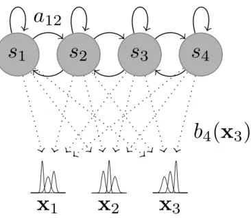
More precisely, as shown in Figure 1.3, each observation or input xt at time step tis
modelled to be emitted, or drawn, from a probability density – the emission probability
bj(xt) =P(xt|st=j), in this case from the GMM – and the transition from state ito
statej is modelled by the so-called transition probabilityaij =P(st=j|st−1 =i).
The above equation can thus also be rewritten as
P(X) =X S∈S as0s1 T Y t=1 bst(xt)ast−1st, (1.12)
with the constraint that s0 be the entry state andsT+1 the exit state.
The GMM that models the emissions takes as input the chosen features from the previous section. Each class is then modelled by a mixture of Gaussians in a multi-dimensional space depending on the feature dimensionality. The Gaussians are defined by a particular parameter set, depending on the number of free parameters: mean, covariances and mixture weights [Rabiner, 1989].
To train this model the Baum-Welch algorithm is widely used, which is an iterative method based on the Expectation Maximisation algorithm that updates the different model parameters through reestimation [Rabiner, 1989, Young et al., 2009].
The final decoding of the sequence is then performed by the Viterbi algorithm [Viterbi, 1967, Young et al., 2009]. This algorithm computes the most likely path through a phoneme sequence, namely the maximum likelihood state sequence. Within the Viterbi
1.4. Combined approaches
s
1
s
2
a
12
s
3
s
4
x
1
x
2
b
4
(
x
3
)
x
3
Figure 1.3 – Sequence modelling with a GMM-HMM system.
decoder, certain constraints of a lexicon (pronunciation model) and/or grammar (language model) can be taken into account.
HMMs have been widely used in speech recognition since they allow easy and efficient modelling of sequences of events by states. For a long time they produced the state-of-the-art results in the field.
In this work the Hidden Markov Model Toolkit HTK [Young et al., 2009] is used for all models involving GMMs and HMMs and the decoding.
1.4
Combined approaches
The traditional GMM-HMM approach was widely used until the emergence of artificial neural networks (ANNs) for automatic speech recognition (ASR). With these, the GMM emission models integrated into the HMM temporal modelling scheme were replaced by such new, improved ‘acoustic-phonetic’ models which led to higher performance [Bourlard and Morgan, 1994]. Whereas in ASR the main use for ANNs was initially these emission models (which was then also repeated with success for visual speech recognition), the bigger impact in this domain was achieved through the developments involving convolu-tional neural networks (CNNs) and other deep learning methods for feature extraction and directly in end-to-end systems.
Σσ +1 y(1k−1) y(2k−1) y(3k−1) y(nk−1) w ( k) 0j w ( k) 1j w(2kj) w (k) 3j w (k) nj σ Pn i=1w (k) ij y (k−1) i +w (k) 0j .. . I1 I2 I3 Input
layer Hidden layers
Output layer
· · · k · · ·
O1
O2
Figure 1.4 – Schematic of an MLP with a sigmoid activation function.
1.4.1 Visual feature extraction
In more recent approaches to VSR, the entire visual feature extraction pipeline has been replaced by specific types of ANNs, usually CNNs or auto-encoders. CNNs are a very common image processing tool nowadays, and they allow to extract features from images. Artificial neural networks have been inspired by biology in the way brains consist of networks of neurons. These artificial neurons receive and pass raw and processed information (signals) from one to another in an often layered network [Bishop, 2006]. Each neuron has the following characteristics: an activation function f(·) that maps the weighted (bywij) inputsxi to a certain output valueyj. These functions are often
nonlinear, following their biological models. In this case and when they contain several layers, these networks can also be referred to as multilayer perceptrons (MLPs). The layers of the network that lie between the input and the output layer are often called
hidden layers since their activations are not observed directly.
The activationa(jk) of neuron j in layerk with inputs y(ik−1) in the preceding layer for i∈ {1,· · ·, n} is given by a(jk)= n X i=1 wij(k)yi(k−1)+wj0, (1.13)
wherew0j is also referred to as the bias.
The output of a neuronj in layer kis then
y(jk) =f(a(jk)), (1.14)
with activation functionf(·) acting on a(jk). Figure 1.4 shows a schematic of an MLP
1.4. Combined approaches ANNs are trained using the backpropagation algorithm which involves the iterative minimisation of a cost, or loss, function. The first stage evaluates the gradient of this cost function with respect to the weights by propagating the error through the network. In the second step the weights are updated by taking into account these derivatives. Generally, this update is limited by a percentage, the learning rate, which controls by
how much each training sample influences the update and is used to regulate the speed of convergence and the risk of overfitting [Bishop, 2006].
Mathematically, the backpropagation of errors is based on the following formula:
δi(k)=f0(ai) n
X
j=1
w(ijk)δj(k+1), (1.15)
where δi(k) is the ‘error’ corresponding to hidden neuron i in layer k and δj(k) are the
‘errors’ associated to the preceding (i.e. closer to the output, since the error is propagated backwards through the network) hidden, or output, neuronsj in layerk+ 1. w(ijk) are the
weights associated to these neurons, andf0(·) is the derivative of the activation function, here evaluated at a(ik). For the output layer, the ‘error’ is calculated directly as the
difference between the ground truthtj and the network outputs oj, i.e. δj =oj−tj. The
‘errors’ are then iteratively passed through the network from one layer to the other. The updates ∆w(ijk) to each weight wij(k) can then be obtained by using the gradient
descent algorithm – a first-order iterative optimisation algorithm to find the minimum of a function –, making small updates in the direction of the negative gradient:
∆w(ijk)=−η ∂E ∂w(ijk) =−ηδ (k) j y (k−1) i , (1.16)
where η is the learning rate andE is the loss function. The update of one sample at a
time is also referred to asstochastic learning, whereas updating after observing a number
(the batch size) of training samples is called batch learning. For the latter, the individual
contributions of each sample in a mini batch are summed up to perform one update after each batch.
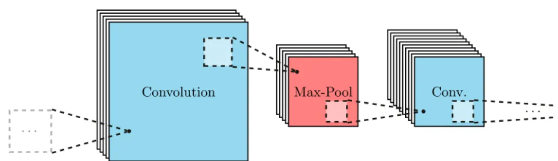
Convolutional neural networks (CNNs) are a specific type of ANN based on the concept of receptive fields. In humans and other animals, neurons in the visual cortex process information from a small, specific region in the field of view, the so-called local receptive field. These can be represented by a weight matrix, usually referred to as a filter or kernel, applied to a particular region. In CNNs the weights are often shared between several neurons of a certain layer, thus allowing to recognise similar shapes across the image and to reduce the number of parameters at the same time. This operation can also be seen as a convolution of the neurons of the local receptive field with the filter [Le Cun et al., 1990]. A major advantage of CNNs over MLPs is the fact that unlike the latter, the former’s layers are often not fully connected, thus significantly reducing both
Convolution Max-Pool Conv. . . .
. . .
Figure 1.5 – Schematic of the basic building blocks of a CNN.
the training time and the need for training data.
In Figure 1.5 an example of two basic building blocks of a CNN is shown: these are the convolutional layers, in which an input is convolved with each neuron’s receptive field, thus creating a new activation matrix for each neuron; and the max pooling layers, which compress the activations by only passing the maximum value for each cluster within a given grid, as shown with a box in Figure 1.5. Another important building block consists in the fully connected layers, which have connections between all neurons, similarly to the neurons in an MLP. The same backpropagation algorithm with gradient descent as mentioned above can be used to train CNNs.
In recent years, deep learning methods with multiple hidden layers between the input and output layers, such as CNNs, have been shown to have superior image and object classification performance [Donahue et al., 2015, Chan et al., 2015] which in turn should also mean that they are better at extracting discriminative features from the image for further processing like in VSR.
In the VSR domain, Ngiam et al. [2011] started by using deep Boltzmann machines for feature extraction in combination with support vector machines to classify the utterances, normalised in length. Other researchers extracted the features with deep belief networks [Huang and Kingsbury, 2013] and CNNs [Noda et al., 2014, Koller et al., 2015].
1.4.2 Sequence modelling
There are multiple ways to use the output of an ANN. One possibility is to simply use the output of these models as an input to the traditional GMM-HMM system, practically like features. This approach is called a tandem system [Hermansky et al., 2000].
However, there is another advantage of using ANNs: Their output represents a probability distribution, which can easily be treated in the subsequent HMM sequence model as the emission probability P(xt|st) if the posterior probabilityP(st|xt) is normalised by the
1.5. Deep learning approaches probability of the state P(st). It thus does not require an additional acoustic model.
These kind of models are the so-called hybrid approaches [Bourlard and Morgan, 1994]. For VSR tandem systems with a GMM-HMM recogniser have been used in several works [Huang and Kingsbury, 2013, Noda et al., 2014, Sui et al., 2015]. Other research has made use of the hybrid approach [Thangthai et al., 2015, Thangthai and Harvey, 2017]. Mroueh et al. [2015] use another type of combined system by using hand-crafted features, based on scattering coefficients and LDA, and then replace the entire recognition system by a bilinear network.
1.5
Deep learning approaches
With the increasing availability of larger datasets and more powerful computational resources, the latest work in VSR has replaced the whole recognition pipeline by recurrent neural networks (RNNs), such as long short-term memories (LSTMs), on top of features extracted from deep neural networks (DNNs) and more specifically CNNs [Wand et al., 2016, Chung et al., 2017, Petridis et al., 2017a]. Thus, VSR has taken advantage of and joined the recent advances in computer vision and speech recognition.
1.5.1 Feature extraction
In these deep learning frameworks, the feature extraction is typically performed using a specific type of neural network, such as an auto-encoder framework, or the CNN described in the previous section. Often it is trained in sequence, within one large network, together with the RNN, thus resulting in an end-to-end deep learning framework. The features are therefore not analysed on their own, but get evaluated through the overall system.
1.5.2 Sequence modelling
Similarly to other types of artificial neural networks, recurrent neural networks are made up of neurons, or cells. However, contrary to those other networks, a given cell in an RNN receives as input not only the activations from other nodes, but also the outputs from a previous sample’s pass through the network, as well as the same cell’s so-called
state from this previous pass. The influence of each of these factors on the cell’s new
output is determined by a set of weights.
The most common type of RNN is made up of long short-term memory (LSTM) cells. In this type of network the cell is comprised of three gates (see Figure 1.6): an input, a forget and an output gate [Hochreiter and Schmidhuber, 1997, Olah, 2015]. At the different gates, the input, the output and the cell state from the previous timestep are weighted with learned matrices. Thus the cell’s new output and state are a function of
these three entry values.
The input gate receives both the current input vectorxt and the previous output vector
yt−1:
it=σ(Wi·[yt−1, xt] +bi), (1.17)
˜
Ct= tanh(WC ·[yt−1, xt] +bC), (1.18)
where·represents a matrix multiplication, here with weight matricesWi, andWC andbi
and bC are the bias terms, of the input gate and candidate value, respectively.
The candidate values ˜Ct are combined with the output from the forget gate ft
ft=σ(Wf·[yt−1, xt] +bf), (1.19)
whereWf is the forget gate’s weight matrix andbf its bias, to produce the new cell state:
Ct=ft∗Ct−1+it∗C˜t, (1.20)
where∗ represents an element-wise multiplication.
Finally, the output gate computes the output weight otand, in combination with the cell
state, gives the new cell output yt:
ot=σ(Wo·[yt−1, xt] +bo), (1.21)
yt=ot∗tanh(Ct), (1.22)
with the output gate’s weight matrixWo and bias bo.
Another important type of RNN is the gated recurrent unit (GRU) [Cho et al., 2014]. Similar to the LSTM, the design of GRUs is based on gates (see Figure 1.7). However, to reduce the number of parameters, the input and forget gates are combined, as are the output and cell states. Furthermore, there is no nonlinearity when computing the output. The lower number of parameters makes it an attractive choice for smaller datasets. In the following, we thus describe the internal workings of a GRU:
The update gatezt at timetdetermines what will be retained from the previous memory
stateyt−1, by also taking into account the current inputxt
zt=σ(Wz·[yt−1, xt]), (1.23)
where·represents a matrix multiplication, here withWz, the update gate’s weight matrix.
1.5. Deep learning approaches ⊗ ⊗ ⊕ ⊗ || xt yt−1 Ct−1 Ct yt yt ft it ˜ Ct ot
Figure 1.6 – Schematic of an LSTM cell.
previous memory:
rt=σ(Wr·[yt−1, xt]), (1.24)
with the reset gate’s weight matrixWr.
The new memory state and the unit’s activation are obtained in two steps. First, the hidden state ˜yt is calculated:
˜
yt= tanh(Wh·[rt∗yt−1, xt]), (1.25)
where ∗represents an element-wise multiplication and Wh is the hidden state’s weight
matrix.
Second, the final current output and cell stateyt is given by
yt= (1−zt)∗yt−1+zt∗y˜t. (1.26)
In visual speech recognition, researchers have used both GRUs [Assael et al., 2016, Xu et al., 2018] and LSTM cells [Chung et al., 2017, Stafylakis and Tzimiropoulos, 2017] successfully to model the temporal evolution. They are trained using gradient descent and backpropagation (see Section 1.4.1).
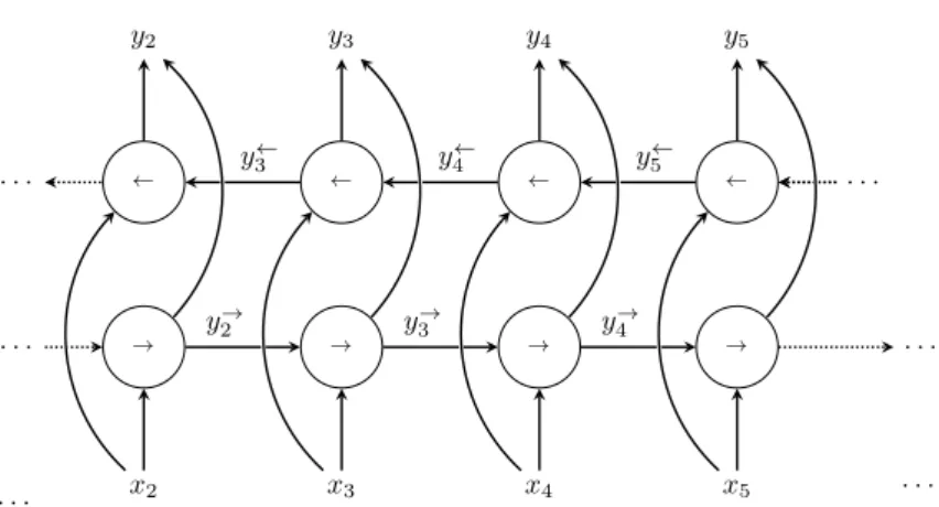
In recent literature, so-called bidirectional RNNs [Schuster and K. Paliwal, 1997] have been employed very often to improve predictability. Each bidirectional layer consists of two recurrent layers which take as input the sequence in its forward and backward direction, as shown in Figure 1.8. This allows learning connections between various
1− ⊗ ⊗ ⊗ ⊕ || || xt yt−1 yt yt rt z t y˜t
Figure 1.7 – Schematic of a GRU.
elements in both directions, taking into account the previous as well as the future contexts [Graves and Jaitly, 2014]. This advantage has been exploited, among others, by Petridis et al. [2017a], Xu et al. [2018].
The work presented in this thesis compares the results of networks with uni- and bidirectional GRUs and LSTM cells.
. . . → → → → . . . ← ← ← ← . . . . x2 x3 x4 x5 y5 y4 y3 y2 y→ 2 y→3 y4→ . . . . y← 3 y4← y5←
1.5. Deep learning approaches
Decoding
The main issue with the RNN outputs is that classification is still framewise whereas the goal in speech recognition is to label a sequence. Similar to the decoding of HMMs using the Viterbi decoder, connectionist temporal classification (CTC) scoring function deter-mines the joint conditional probability of an overall sequence at given timestamps [Graves, 2008]. In doing so, it functions as an additional layer that can receive as input the framewise output from the bidirectional GRU or LSTM of a certain (variable) length and can output a sequence of symbols (in our case phonemes or visemes, the visual equivalent) of a different (variable) length. For this, CTC does not require time-aligned labels – the overall sequence is sufficient, meaning that it does not depend on the accuracy of the labelling of the training set. The output will also only reflect the overall sequence, and not be evaluated by its timings.
Similarly to HMMs, the CTC algorithm will need to add an extra “blank” class to the labels. This class “collects” all types of silence or other non-speech occurrences in the utterance. It will generally appear between labels which can also help in case of the consecutive occurrence of the same label.
In mathematical terms, the decoding of the network can be described by the maximisation of the following function [Graves and Jaitly, 2014]:
arg max
Y P(Y|X)≈B(arg maxS P(S|X)), (1.27) where the input sequence X is transcribed by the label sequence Y. This can be approximated by using the alignmentS, related to the transcriptionY through the sum of all possible alignments or states S,
P(Y|X) = X
S∈B−1(Y)
P(S|X), (1.28)
where the operatorB removes all repeated labels and blanks.
The probability of the alignment itself is the combined probability of the emission probabilities of the alignments st at all time stepst∈ {1, . . . , T} which, assuming their
independence, is given by:
P(S|X) =
T
Y
t=1
P(st, t|X). (1.29)
Decoding can be performed either in a greedy manner, using best path decoding, or by taking into account all possible sequences, using prefix search decoding. Best path
decoding finds the particular path with the highest probability: S∗= arg max S T Y t=1 P(st, t|X), (1.30)
whereS are the possible alignments andS∗ is the most probable alignment.
However, this method does not take into account the fact that there might exist several paths which – through repetitions of symbols or intermediate blanks – are ultimately identical. Prefix search decoding also considers these similar paths – which in turn increases the search space exponentially with the length of the input sequence. If certain conditions – such as sufficiently peaked output distributions, or an adapted beam search to only take into account the more promising paths, or additional constraints through a language model – are met, then prefix search decoding still remains feasible [Graves et al., 2006, Hannun, 2017].
Training of the CTC layer functions similarly to HMM training with a forward-backward algorithm based on maximum likelihood. Therefore, the aim is to minimise the objective function based on the negative log probability that the whole training set Z is labelled
correctly (with target transcriptions Y∗):
O(Z,Nw) =−
X
(X,Y∗)∈Z
ln(P(Y∗|X)), (1.31)
whereNw is the neural network to be trained [Graves et al., 2006]. It is thus indirectly
also related to the edit distance or label error rate (see Section 1.6).
When using gradient descent in the training step to update the network with the help of the commonly used backpropagation algorithm (see Section 1.4.1), the derivative of this objective function with respect to the network output has to be taken (see [Graves et al., 2006] for more details).
Other methods for sequence decoding of network outputs have been developed in recent years. One of these decoding methods uses an RNN transducer built on top of a CTC. It combines the CTC-style network with another, separate RNN which acts as a joint acoustic and language model to predict each phoneme given the previous ones [Graves et al., 2013]. This thus results in additional hidden layers for the CTC network, and increases the number of parameters of the model.
While in audio speech recognition these sequence modelling techniques for RNNs have been widely used for several years, they are relatively new in VSR. CTC has been used by Assael et al. [2016], Koumparoulis et al. [2017], Xu et al. [2018].
Another recent sequence modelling technique is the so-called attention scheme [Bahdanau et al., 2016, Chan et al., 2016] for encoder-decoder based systems. It acts between the
1.6. Performance metrics encoder and decoder as a sort of weighting which depends on a normalised score of the previous state, the current encoded sequence and the convolutional features. A language model can still be added with final state transducers or in the beam search. Some more recent work combines both CTC and the attention scheme [Kim et al., 2017, Xu et al., 2018].
The work presented in this thesis uses the CTC scheme for sequence decoding since this scheme fits best with the CNN-RNN network and the database used.
1.6
Performance metrics
In this thesis, two metrics are used to present the results: the accuracy and correctness at the viseme or word level, and the percentage of correct sentences. The accuracy and correctness are defined as follows
Accuracy= H−I
N ·100%, (1.32)
Correctness= H
N ·100%, (1.33)
whereH, I, and N are the number of correct symbols (visemes or words), number of
erroneous symbols (insertion error), and the total number of symbols in the reference, respectively. The number of correct symbols is equal to the number of all symbols minus the total number of ignored symbols (deletion error, D) and the number of wrongly
recognised symbols (substitution error, S), i.e. H = N −D−S. The accuracy also
penalises insertions and is thus related to the edit distance, given by I+D+S.
Some of the literature evaluates speech recognition results in terms of another metric related to the edit distance: the word error rate (WER) – or sometimes phoneme/label error rate – rather than the accuracy, which can be obtained from the word accuracy in the following way:
WER= I+D+S
N ·100% = 100%−Accuracy. (1.34)
1.7
Multi-view visual speech recognition
While audio-based speech recognition has improved significantly over the past decades and is nowadays applicable in many real-life scenarios, visual speech recognition still mostly focuses on speech produced in controlled lab conditions. However, there is a lot of interest to address, for example, the problem of head pose, which is a large hindrance in the application to real-world scenarios. Early work on multi-pose or non-frontal automatic lip reading focused on using classifiers for each different head pose and defining
a linear transformation or the regression of appearance-based features such as the DCT or a subsequently applied LDA [Lucey et al., 2007, Estellers and Thiran, 2012]. Other researchers worked on cross-view training/testing, i.e., training on one view and testing on another [Lan et al., 2012]. Lan et al. [2012] also established that the 30◦ view angle
provides the best recognition performance, even over the frontal view. Some recent research has applied cross-view analysis to 3D-AAMs [Watanabe et al., 2017] and used channel, image and feature fusion for multiple- and cross-view analysis [Lee et al., 2017]. In [Bowden et al., 2013], three different view angles are explored. Two ways to detect this angle are tested: (i) smallest root-mean-square error of three face trackers for each angle, and (ii) shortest distance of the local gradient orientation (LGO) histogram which performs better since it does not depend on the tracker results.
A method to remove off-plane head rotation has been used by Koller et al. [2014]. Here the shape is registered to a frontal view with a 3D point density model (PDM) trained with a non-rigid structure-from-motion algorithm. However, it is not clear up to which view angles this algorithm is functional. Watanabe et al. [2017] use 3D-AAMs for the same purpose of cross-view VSR.
Nowadays, in many applications, such as driver monitoring, the advantages of using several cameras to cover a larger field of view outweigh the cost of systems with multiple cameras and additional computational resources. Several cameras thus allow to integrate the views to have more confident results, as well as a larger variety of head poses. Recently, several researchers in this field have also joined different views at various levels of the processing pipeline. In Navarathna et al. [2013], a synchronous HMM was built to include four different views (centre left, centre right, side left, side right). The weights for this multi-stream HMM are determined empirically by comparing the training performance between the centre and the side views and the left and right views for varying weights. The final individual weights are a combination of these coarser weights. Lee et al. [2017], Petridis et al. [2017b] use the OuluVS2 database with five different views [Anina et al., 2015]. Lee et al. [2017] use a combination of CNNs and LSTMs with a final layer that provides the probability that one out of ten different phrases has been uttered. They show results for different types of combinations: 3D-CNN, merging channels, merging images and concatenating features at the output of the CNN. Finally, Petridis et al. [2017b] propose an end-to-end deep learning system made up of restricted Boltzmann machines (RBMs) and bidirectional LSTMs (BLSTMs) where the views are fused between two layers of the BLSTM. They also provide a comparison between the multi-view results from several researchers. Also in the latter system classification is performed at the sentence-level.