Spatio-Temporal Saliency Detection in Dynamic Scenes
using Local Binary Patterns
Satya Muddamsetty, D´
esir´
e Sidib´
e, Alain Tr´
emeau, Fabrice Meriaudeau
To cite this version:
Satya Muddamsetty, D´
esir´
e Sidib´
e, Alain Tr´
emeau, Fabrice Meriaudeau.
Spatio-Temporal
Saliency Detection in Dynamic Scenes using Local Binary Patterns. ICPR, Aug 2014,
Stock-holm, Sweden. pp.1-6, 2014.
<
hal-00995334
>
HAL Id: hal-00995334
https://hal-univ-bourgogne.archives-ouvertes.fr/hal-00995334
Submitted on 23 May 2014
HAL
is a multi-disciplinary open access
archive for the deposit and dissemination of
sci-entific research documents, whether they are
pub-lished or not.
The documents may come from
teaching and research institutions in France or
abroad, or from public or private research centers.
L’archive ouverte pluridisciplinaire
HAL
, est
destin´
ee au d´
epˆ
ot et `
a la diffusion de documents
scientifiques de niveau recherche, publi´
es ou non,
´
emanant des ´
etablissements d’enseignement et de
recherche fran¸cais ou ´
etrangers, des laboratoires
publics ou priv´
es.
Spatio-Temporal Saliency Detection in Dynamic
Scenes using Local Binary Patterns
Satya M. Muddamsetty
∗, D´esir´e Sidib´e
∗, Alain Tr´emeau
†and Fabrice M´eriaudeau
∗∗Le2i UMR CNRS 6306, Universit´e de Bourgogne, 12 rue de la fonderie, 71200 Le Creusot, France †Laboratoire Hubert Curien UMR CNRS 5116, Universit´e Jean Monnet
Abstract—Visual saliency detection is an important step in many computer vision applications, since it reduces further processing steps to regions of interest. Saliency detection in still images is a well-studied topic. However, videos scenes contain more information than static images, and this additional tem-poral information is an important aspect of human perception. Therefore, it is necessary to include motion information in order to obtain spatio-temporal saliency map for a dynamic scene. In this paper, we introduce a new spatio-temporal saliency detection method for dynamic scenes based on dynamic textures computed with local binary patterns. In particular, we extract local binary patterns descriptors in two orthogonal planes (LBP-TOP) to describe temporal information, and color features are used to represent spatial information. The obtained three maps are finally fused into a spatio-temporal saliency map. The algorithm is evaluated on a dataset with complex dynamic scenes and the results show that our proposed method outperforms state-of-art methods.
I. INTRODUCTION
Visual saliency intuitively characterizes parts of a scene which stand out relative to their neighbouring parts, and immediately grab an observer’s attention. It is an important and fundamental research problem in neuroscience and psychology to investigate the mechanism of human visual system in selecting regions of interest in complex scenes. It has been an active research topic in computer vision research due to various applications such as object detection [1], image segmentation [2], robotic navigation and localization [3], video surveillance [4], object tracking [5], image re-targeting [6] and image/video compression [7].
According to psychological studies [8], visual attention process follows two basic principles: bottom-up and top-down approaches. Bottom-up approach is a task independent process derived solely from the visual input. Regions which attract attention in a bottom-up way are called salient and the responsible features should be sufficiently discriminative with respect to the surrounding regions. In top-down approaches, the attention is driven by cognitive factors such as knowledge, expectations and current goals. Among these two categories, bottom-up mechanism has been more investigated than top-down mechanism, since data-driven stimuli are easier to con-trol than cognitive factors [8].
Different theories have been proposed to explain and better understand human perception. The feature integration theory
(FIT) [9] and the guided search model [10] are the most influential ones. In FIT, the visual information is analyzed in parallel from different feature maps. Based on FIT, Koch and Ullman [11] have proposed the first neurally plausible
architecture. In their framework, different feature maps using low level features such as color, intensity, orientation, motion, texture and spatial frequency are computed in parallel and the conspicuity of every pixel in an image are represented in a topographic representation known as saliency map. Most of existing bottom-up approaches follow the same architecture. In theguided search model, the goal is to explain and predict the results of visual search experiments. This model considers top-down process along with bottom-up saliency to distinguish the target from the distractors.
Several methods have been proposed to detect salient regions in images and videos, and a recent survey of state-of-art methods can be found in [12]. However, most of these methods are limited to static images and few attention has been given to videos. Dealing with videos is more complicated than static images and the perception of video is also different from that of static images due to additional temporal information. A video shows a strong spatio-temporal correlation between the regions of consecutive frames. A common approach to deal with video sequences is to compute a static saliency map for each frame and to combine it with a dynamic map to get the final spatio-temporal saliency map. The accuracy of the saliency model depends on the quality of both the static and dynamic saliency maps and also on the fusion method as shown in [13].
Most of the existing spatio-temporal saliency models [4], [14], [13] use optical flow methods to process the motion information. In these methods, motion intensity of each pixel is computed and the final saliency map represents the pix-els which are moving against the background. Optical flow based methods can work when the scene studied has simple background and fail with complex background scenes. Real world scenes are composed of several dynamic entities such as moving trees, moving water, snow, rain, fog and crowds. This makes the scene background very complex whereas optical flow based methods cannot compute accurate dynamic saliency maps.
To address these limitations, we propose a new spatio-temporal saliency detection method in this paper. Our method is based on local binary patterns (LBP) for representing the scene as dynamic textures. The dynamic textures are modeled using local binary patterns in orthogonal planes (LBP-TOP) which is an extension of the LBP operator in temporal di-rection [15]. Our contributions are twofold. First, we apply a center-surround mechanism to the extracted dynamic textures in order to obtain a measure of saliency in different directions. Second, we propose to combine color and texture features from which the spatial saliency map is computed using color
features meanwhile the temporal saliency map is computed using dynamic textures from LBP in two orthogonal planes. The different saliency maps are finally fused to obtain the final spatio-temporal saliency map.
The rest of the paper is organized as follows. In Section II, we review some of the spatio-temporal saliency detection methods presented in literature. In Section III, we describe the proposed LBP-TOP based spatio-temporal saliency model. Section IV, shows performance evaluation of our methods and comparison with other approaches. Finally, Section V gives concluding remarks.
II. RELATEDWORK
In this section, we briefly introduce some of the saliency models described in literature. All these methods follow the bottom-up approach principles. Itti et al. [16] proposed the first biologically inspired saliency model. In their method, the authors used a set of feature maps such as intensity, color and orientation, which are normalized and linearly combined to generate the overall saliency map. Even if this model does not deal with any motion information, it has become a benchmark model for the other models. In [1], authors proposed an information theoretic spatio-temporal saliency model which is computed from spatio-temporal volumes. Marat et al.[14] proposed a space-time saliency algorithm which is inspired by the human visual system. First, a static saliency map is computed using color features, and a dynamic saliency map is computed using motion information derived from optical flow. The two maps are then fused to generate space-time saliency map. In a similar way, Tong et al. [4] proposed a saliency model which is used for video surveillance. The spatial map is computed based on low level features and the dynamic map is computed based on motion intensity, motion orientation and phase.
A phase spectrum approach is proposed by Guo and Zhang [7]. In this method, motion is computed by taking the difference between two frames, and is combined with color and intensity. The features are put together using a quaternion representation and Quaternion Fourier Transform (QFT) is applied to get final saliency map. Kim et al. [17] presented a salient region detection method for both images and videos based on center-surround hypothesis. They used edge and color orientations to compute the spatial saliency. The dynamic saliency is computed by taking the absolute difference between the center and surround temporal gradients and is finally fused with the spatial map. Zhouet al. [18] proposed a dynamic saliency model to detect moving objects against dynamic backgrounds. In this algorithm, the displacement of foreground and background objects are represented by the phase change of Fourier spectra and the saliency map is generated using the displacement vector. In [19], Seo and Milanfar proposed a unified space-time saliency detection in which they compute local regression kernels from the image or video and finally measure the likeness of pixel or (voxel) to its surroundings. Saliency is then detected based on a measure of self-resemblance computed using cosine similarity. A similar method is developed in [20], where the video patches are modeled using dynamic textures and saliency is computed based on discriminant center-surround.
Most of these methods fail to address complex scenes. In particular, methods based on optical flow fail to compute ac-curate dynamic saliency maps for scenes with highly textured backgrounds.
III. PROPOSEDSPATIO-TEMPORALSALIENCY
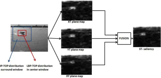
In this section, we introduce our proposed spatio-temporal saliency detection method for dynamic scene based on local binary patterns. In particular, we model dynamic textures using local binary patterns computed in orthogonal planes (LBP-TOP) and apply a center-surround mechanism to compute a saliency measure in different directions. Then, we combine the spatial saliency map computed using color features and the temporal saliency map computed using dynamic textures, to obtain the final spatio-temporal saliency map. An overview of the method is presented in Fig. 1, and the different steps are described in the following subsections.
A. Modeling dynamic textures using LBP-TOP
Dynamic or temporal textures are textures that show stationary properties in time. They encompass the different difficulties mentioned in the introduction (Section??) such as moving trees, moving water, snow, rain, fog, etc. Therefore, we adopt dynamic textures to model the varying appearance of dynamic scenes with time. Several approaches have been developed to represent dynamic textures and a review can be found in [21].
In our work, we use the LBP-TOP approach of Zhao and Pietik¨ainen [15]. LBP-TOP is an extension of local binary patterns (LBP) that combines both motion and appearance features simultaneously and has been used for applications such as facial expression analysis [15] or human activity recognition [22].
In its simplest form, LBP is a texture operator which labels the pixels of an image by thresholding the neighbourhood of each pixel and considers the result as a binary number [23]. The original LBP operator is based on a circular sampling:
LBP(xc, yc) = P X p=1 s(gp−gc) 2p, s(x) ={1, x≥00, x <0, (1) wheregc is the gray value of the center pixel (xc, yc)andgp are the gray values at the P sampling points in the circular neighbourhood of(xc, yc).
The LBP-TOP operator extends LBP to temporal domain by computing the co-occurrences of local binary patterns on three orthogonal planes such as XY, XT and YT. The XT and YT planes provide information about the space-time transitions and the XY plane provides spatial information. These three orthogonal planes intersect at the center pixel. LBP-TOP considers the feature distributions from each separate plane and then concatenates them into a single histogram. The circular neighborhoods are generalized to elliptical sampling to fit to the space-time statistics [15].
B. Spatio-temporal saliency detection using LBPTOP descrip-tor
After modeling dynamic textures using LBP-TOP, we com-pute spatio-temporal saliency using a center-surround (CS)
Fig. 1. Overview of the proposed spatio-temporal saliency detection method.
mechanism. CS is a discriminant formulation in which the features distribution of the center of visual stimuli is compared with the feature distribution of surrounding stimuli.
For each pixel location l = (xc, yc), we extract a center regionrC and a surrounding regionrS both centered atl. We set the size of the surrounding region to be six time larger than the center region. We then compute the feature distributionshc andhs of both regions as histograms and define the saliency of pixell as the dissimilarity between these two distributions. More specifically, the saliency S(l) of pixel at location l is given by: S(l) =χ2(hc,hs) = B X i=1 (hc(i)−hs(i))2 (hs(i) +hc)/2 , (2)
where hc and hs are the histograms distributions of rC and
rS respectively,Bis the number of bins of the histogram, and
χ2 is the Chi-square distance measure.
Note that we separately apply center-surround mechanism to each of the three planes XY, XT and YT. Hence, we compute three different saliency maps based on the three distributions derived from LBP-TOP.
The final step of the method consists in fusing the previous three maps into a single spatio-temporal saliency map. This is done in two steps. First, the two maps containing temporal information, i.e. the saliency maps from XT and YT planes, are fused to get a dynamic saliency map. Then, this dynamic saliency map is fused with the static saliency map from the XY plane. As shown in [13], the fusion method affects the quality of the obtained final spatio-temporal saliency map. In this work, we employ the Dynamic Weighted Fusion(DWF) scheme as it has shown best performance in a recent evaluation of different fusion techniques [13]. In DWF the weights are calculated by computing a ratio between the means of both the maps to combine, so they are updated from frame to frame. LetSXT andSY T be the saliency maps obtained from the XT and YT planes respectively. They are fused into a dynamic saliency mapMD as follows:
MD=αDSY T + (1−αD)SXT, (3) whereαD= mean(Smean(SY T)
XT)+mean(SY T).
The obtained dynamic mapMD and the static mapMS=
SXY are fused in a similar manner.
C. Combining color and dynamic textures features
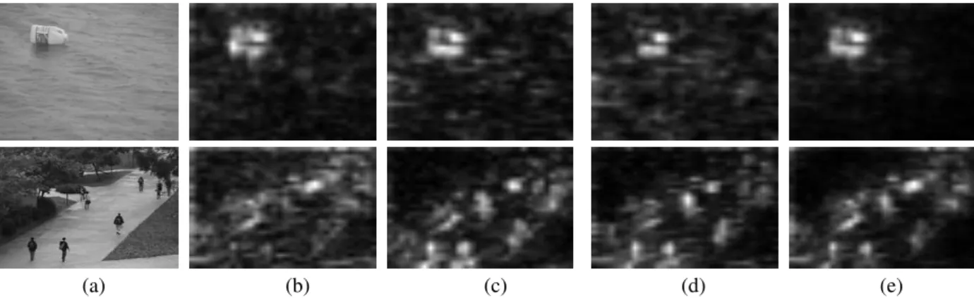
We observe that the spatial saliency map derived from the XY plane fails to highlight salient objects of some scenes because LBP-TOP does not use color features. Figure 2 shows examples of saliency maps obtained from LBP-TOP features. As it can be seen in the second column of Fig. 2, the saliency map obtained in the XY plane fails to highlights objects of interest, for example the moving persons in the second row of the figure.
This observation motivates us to replace the LBP features computed in XY plane by color features and compute the spatial saliency map following the context-aware method of Gofermanet al.[24] since this saliency detection method was shown to achieve best performance in a recent evaluation [25].
1) Spatial Saliency: The spatial saliency is computed based on context aware saliency. In this method the salient regions should not only contain the prominent objects but also the parts of the background which convey the context [24]. It is based on the distinctiveness of a region with respect to both its local and global surroundings.
In a first step a local single-scale saliency is computed for each pixel in the image. The dissimilarity measure between a pair of patches is defined by:
d(pi, qk) =
dcolor(pi, qk) 1 +c.dposition(pi, qk)
, (4)
wheredcolor(pi, qk) is the Euclidean distance between image patchespiand{qk}
K
k=1, of patch size7×7, centered at pixeli
andk, whereK is the number of the most similar patches (if the most similar patches are highly different frompi, then all image patches are highly different frompi) in CIELAB color space.dposition(pi, qk)is the Euclidean distance between the positions of patchespi andqk andc is a constant scalar value set to c = 3 in our experiments (changing the value to any smaller scalar value produces slight change in the saliency
(a) (b) (c) (d) (e)
Fig. 2. Examples of spatio-temporal saliency detection with LBP-TOP features. (a) Original frame; (b) saliency map in XY plane; (c) saliency map in XT plane; (d) saliency map in YT plane; (e) fused spatio-temporal saliency map.
map but the final result is almost identical). The single-scale saliency value of pixeliat scaler is then defined as:
Sr i = 1−e− 1 K PK k=1d(p r i,q r k). (5)
In a second step, a pixel is considered salient if itsKmost similar patches{qk}
K
k=1at different scales are significantly
dif-ferent from it. The global saliency of a pixeliis characterized by the mean of its saliency at different scales.
The final step includes the immediate context of the salient object. The visual contextual effect is simulated by extracting the most attended localized areas at each scale. A pixel i
is considered as a focus of attention at scale r which is normalized to the range [0, 1], if the dissimilarity measure of Eq. 4 exceeds a given threshold (Sr
i > 0.8). Then, each pixel which is outside of attended areas is weighted according to its Euclidean distance to the closest focus of attention pixel. The final saliency map which includes the context information is computed as: ˆ Si= 1 M X sr i(1−d r f oci(i)), (6) where M is the total number of scales and df oci(i) is the Euclidean positional distance between pixeli and the closest focus of attention pixel at scaler.
2) Temporal Saliency: The temporal saliency map is com-puted using dynamic textures from LBP-TOP features in the XT and YT planes. The two maps, one for each plane, are fused into a single dynamic saliency map using the DWT fusion scheme explained in Section III-B.
3) Post-processing: After obtaining the spatial and tempo-ral saliency maps, respectively MS and MD, both are fused into the final spatio-temporal saliency map as:
MDS =αMD+ (1−α)MS, (7) withα= mean(MD)
mean(MD)+mean(MS).
The last step of our method consists in applying a post-processing scheme with the goal of suppressing isolated pixels or group of pixels with low saliency values. We start by finding pixels whose saliency value is above a defined threshold (0.5 in our experiments, the final saliency mapMDSbeing normalized to have values in[0,1]). Then, we compute the spatial distance
D(x, y)from each pixel to the nearest non-zero pixel in the thresholded map. The spatio-temporal saliency map MF is finally refined using the following equation:
MF(x, y) =e
−D(x,y)
λ ×MDS(x, y), (8)
whereλis a constant set toλ= 0.5. The influence of this last parameter is studied in the next section showing experimental results.
IV. EXPERIMENTS ANDRESULTS
In this section, we evaluate the performance of the pro-posed saliency detection method using LBP features on a publicly available dataset of dynamic scenes [20]. The dataset contains twelve video sequences with dynamic background scenes such as moving trees, snow, smoke, fog, pedestrians, waves in the sea and moving cameras. For each sequence, a manual segmentation of the salient objects is available for every frame and served as ground truth. This allows us to perform a quantitative analysis of the methods performance.
We compare the proposed spatio-temporal saliency detec-tion method combining color features and LBP-TOP features (PROPOSED), with the method using LBP features only (LBP-TOP) and three state-of-art methods: a method using optical flow to compute motion features (OF) [13], the self-resemblance method (SR) [19] and the phased discrepancy based saliency detection method (PD) [18]. For the last three methods, we use codes provided by the authors. For LBP-TOP based saliency, we use center-surround mechanism described in Section III-B with a center region of size 17×17 and a surround region of size97×97, and we extract LBP features from a temporal volume of six frames.
We evaluate the different spatio-temporal saliency detec-tion methods by generating Receiver Operating Characteristic (ROC) curves and evaluating the Area Under ROC Curve (AUC). For each method, the obtained spatio-temporal saliency map is first normalized to the range [0, 1], and binarized using a varying threshold t ∈ [0,1]. With the binarized maps, we compute the true positive rate and false positive rate with respect to the ground truth data.
The post-processing step described in Section III-C is important in order to obtain good final saliency maps. It basically lower the final saliency value of pixels far away
Fig. 3. Influence ofλon the proposed method performance.
from all pixels with saliency value above a defined threshold. The parameter λ in Eq. (8) controls the importance of the attenuation. The effect of this parameter can be observed in Fig. 3 for three sequences. As can be seen, optimal values are between 0.2 and 0.6 for the three sequences. We have selected the value λ = 0.5 as it is in average the best value for all tested sequences.
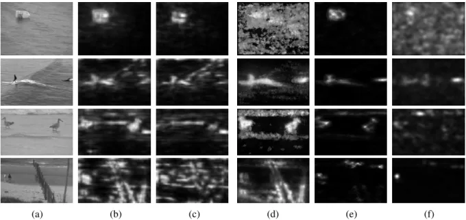
Table I summarizes the results obtained with all sequences by the different saliency detection methods whereas the visual comparison of these methods are shown in Fig. 7. We can observe that the proposed method achieves the best overall performance with an average AUC value of 0.914 for all twelve sequences. The optical flow based method (OF) achieves an average AUC value of 0.907, whereas as self-resemblance (SR), phase discrepancy (PD) and LBO-TOP achieve lower average AUC values, respectively 0.843, 0.837 and 0.745. These results confirm the observation from Section III-C that the combination of color features with LBP features produces better saliency map. In fact, the proposed method fusing color and LBP features gives an average AUC value which is 22% higher that the value wih LBP-TOP features.
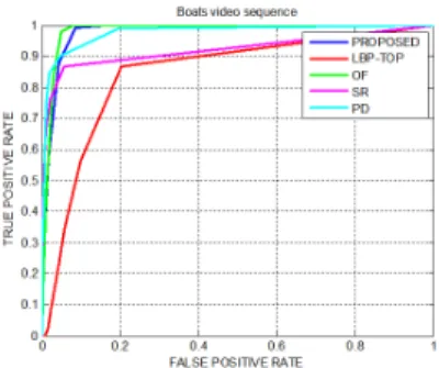
Analyzing the sequences individually, we see that the best and least performances are obtained with theBoats and
Freewaysequences, respectively, with average AUC values of 0.9394 and 0.7398 for all five saliency detection methods. The Boats sequence shows good color and motion contrasts, so both static and dynamic maps are estimated correctly, and all spatio-temporal saliency detection methods perform well. Note however that the LBP-TOP based method gives slightly lower accuracy than other techniques. On the other hand, the color contrast of the Freeway sequence is very limited. So getting a correct static saliency map is difficult with this sequence whereas the quality of the final spatio-temporal saliency map relies on the dynamic map. The best performing method with this sequence is the LBP-TOP based technique with an average AUC value of 0.868, while optical-flow based technique achieves an average AUC value of only 0.545. This example illustrates that using LBP features to rep-resent dynamic textures (and to compute the dynamic saliency map) gives very good results. The ROC curves comparing performances of the different methods on three sequences are shown in Fig. 4,5 and 6.
V. CONCLUSION
In this paper, we have proposed a spatio-temporal saliency detection method of dynamic scenes based on local binary patterns. The method combines in a first step color features for static saliency detection, and dynamic textures for temporal
Fig. 4. Quantitative comparision withBoatssequence.
Fig. 5. Quantitative comparision withFreewaysequence.
Fig. 6. Quantitative comparision withOceansequence.
dynamic saliency detection. The obtained two saliency maps are in a second step fused into a spatio-temporal map. Exper-imental results show that our method performs significantly better than using LBP features alone, and also better than other state-of-art methods. The proposed method is in particular, able to deal with complex dynamic scenes showing difficult background textures.
REFERENCES
[1] L. Chang, P. C. Yuen, and G. Qiu, “Object motion detection using information theoretic spatio-temporal saliency,”Pattern Recogn. 2009, vol. 42, no. 11, pp. 2897–2906.
[2] R. Achanta, F. Estrada, S. Susstrunk, and S. Hemami, “Frequency-tuned salient region detection,”CVPR, 2009, pp. 1597–1604.
[3] C. Siagian and L. Itti, “Biologically inspired mobile robot vision localization,” IEEE Trans on Robotics, vol. 25, no. 4, pp. 861–873, 2009.
[4] T. Yubing, F. A. Cheikh, F. F. E. Guraya, H. . Konik, and A. Trmeau, “A spatiotemporal saliency model for video surveillance,” Cognitive Compuation,2011, vol. Volume 3, Issue 1, pp. 241–263.
[5] D. Sidib´e, D. Fofi, and F. M´eriaudeau, “Using visual saliency for object tracking with particle filters,” inEUSIPCO, 2010.
Sequence PROPOSED LBP-TOP OF [13] SR [19] PD [18] Avg AUC Birds 0.9586 0.7680 0.9664 0.9379 0.8221 0.8906 Boats 0.9794 0.8358 0.9827 0.9227 0.9765 0.9394 Bottle 0.9953 0.9413 0.8787 0.9961 0.8285 0.9279 Cyclists 0.9317 0.6737 0.9602 0.8682 0.9551 0.8777 Chopper 0.9717 0.9427 0.9850 0.7447 0.6470 0.8582 Freeway 0.7775 0.8684 0.5456 0.7760 0.7318 0.7398 Peds 0.9552 0.7376 0.9512 0.8603 0.8548 0.8718 Ocean 0.9271 0.8513 0.7810 0.8016 0.8235 0.8369 Surfers 0.9674 0.7489 0.9545 0.9455 0.9352 0.9103 Skiing 0.8389 0.3787 0.9796 0.8872 0.9367 0.8042 Jump 0.8957 0.6960 0.9481 0.8321 0.6616 0.8067 Traffic 0.7693 0.6088 0.9615 0.5491 0.8720 0.7521 Avg AUC 0.9140 0.7453 0.9079 0.8434 0.8371
TABLE I. EVALUATION OF SPATIO-TEMPORAL SALIENCY DETECTION METHODS. PROPOSED (WITH COLOR ANDLBPFEATURES), LBP-TOP (LBP
FEATURES ONLY), OF (OPTICALFLOW BASED), SR (SELF-RESEMBLANCE)ANDPD (PHASEDISCREPANCY).
(a) (b) (c) (d) (e) (f)
Fig. 7. Visual comparison of spatio-temporal saliency detection of our methods and state of art methods. (a) Original frame; (b) PROPOSED; (c) LBP-TOP; (d) OF [13]; (e) SR [19] and (f) PD [18]
[6] T. Lu, Z. Yuan, Y. Huang, D. Wu, and H. Yu, “Video retargeting with nonlinear spatial-temporal saliency fusion,” inICIP,2010.
[7] C. L. Guo and L. M. Zhang, “A novel multiresolution spatiotemporal saliency detection model and its applications in image and video compression,”IEEE TIP, vol. 19, no. 1, pp. 185 –198, 2010. [8] S. Frintrop,Computational Visual Attention. Springer, 2011. [9] A. M. Treisman and G. Gelade, “A feature-integration theory of
attention.”Cognitive psychology, vol. 12, no. 1, pp. 97–136, 1980. [10] J. M. Wolfe, “Guided search 2.0: A revised model of visual search,”
Psychonomic Bulletin & Review, vol. 1, no. 2, pp. 202–238, 1994. [11] C. Koch and S. Ullman, “Shifts in selection in visual attention:toward
the underlying neural circuitry,”Human Neurobiology, vol. vol. 4, no. 4, pp. 219–27, 1985.
[12] A. Borji and L. Itti, “State-of-the-art in visual attention modeling,”IEEE Trans on PAMI,, vol. 35, no. 1, pp. 185–207, 2013.
[13] S. M. Muddamsetty, D. Sidib´e, A. Tr´emeau, and F. M´eriaudeau, “A performance evaluation of fusion techniques for spatio-temporal saliency detection in dynamic scenes,” inICIP, 2013.
[14] S. Marat, T. H. Phuoc, L. Granjon, N. Guyader, D. Pellerin, and A. Gu´erin-Dugu´e, “Modelling spatio-temporal saliency to predict gaze direction for short videos,”IJCV,2009, vol. 82, no. 3, pp. 231–243. [15] G. Zhao and M. Pietik¨ainen, “Dynamic texture recognition using local
binary patterns with an application to facial expressions,”IEEE Trans on PAMI, vol. 29, no. 6, pp. 915–928, 2007.
[16] L. ltti, C. Koch, and E. Neibur, “A model of saliency-based visual
attention for rapid scene analysis,”IEEE Trans on PAMI,1998, vol. 20, pp. 1254–1259.
[17] W. Kim, C. Jung, and C. Kim, “Spatiotemporal saliency detection and its applications in static and dynamic scenes,” IEEE Trans. Circuits Syst. Video Techn,2011, vol. 21, no. 4, pp. 446–456.
[18] B. Zhou, X. Hou, and L. Zhang, “A phase discrepancy analysis of object motion,” inProc of the 10th ACCV, 2011, pp. 225–238.
[19] H. J. Seo and P. Milanfar, “Static and space-time visual saliency detection by self-resemblance,”Journal of vision, vol. 9, no. 12, 2009. [20] V. Mahadevan and N. Vasconcelos, “Spatiotemporal saliency in dynamic
scenes,”IEEE Trans on PAMI,, vol. 32, no. 1, pp. 171 –177, 2010. [21] D. Chetverikov and R. Peteri, “A brief survey of dynamic texture
description and recognition,” inProc. Intl Conf. Computer Recognition Systems, 2005, pp. 17–26.
[22] P. Crook, V. Kellokumpu, G. Zhao, and M. Pietikainen, “Human activity recognition using a dynamic texture based method,” inProc of the BMVC, 2008, pp. 88.1–88.10.
[23] M. Pietik¨ainen, G. Zhao, A. Hadid, and T. Ahonen,Computer Vision Using Local Binary Patterns, ser. Computational Imaging and Vision. Springer, 2011, no. 40.
[24] S. Goferman, L. Zelnik-manor, and A. Tal, “Context-aware saliency detection,” inIEEE Conf. on CVPR,2010.
[25] A. Borji, N. D. Sihite, and L. Itti, “Salient object detection: A bench-mark,” inECCV (2), 2012, pp. 414–429.