for Pattern Mining from Utility Usage Data
Saad Mohamad, Damla Arifoglu, Chemseddine Mansouri, and Abdelhamid Bouchachia
Department of Computing, Bournemouth University, Poole, UK {smohamad, darifoglu, cmansouri, abouchachia}@bournemouth.ac.uk
Abstract. Non-intrusive load monitoring (NILM) has been tradition-ally approached from signal processing and electrical engineering per-spectives. Recently, machine learning has started to play an important role in NILM. While much work has focused on supervised algorithms, unsupervised approaches can be more interesting and of more practical use in real case scenarios. More specifically, they do not require labelled training data to be collected from individual appliances and the algo-rithm can be deployed to operate on the measured aggregate data di-rectly. In this paper, we propose a fully unsupervised NILM framework based on Deep Belief network (DBN) and online Latent Dirichlet Allo-cation (LDA). Firstly, the raw signals of the house utilities are fed into DBN to extract low-level generic features in an unsupervised fashion, and then the hierarchical Bayesian model, LDA, learns high-level fea-tures that capture the correlations between the low-level ones. Thus, the proposed method (DBN-LDA) harnesses the DBN’s ability of learning distributed hierarchies of features to extract sophisticated appliances-specific features without the need of precise human-crafted input rep-resentations. The clustering power of the hierarchical Bayesian models helps further summarise the input data by extracting higher-level infor-mation representing the residents’ energy consumption patterns. Using Deep-Hierarchical models reduces the computational complexity since LDA is not directly applied to the raw data. The computational effi-ciency is crucial as our application involves massive data from different types of utility usages. Moreover, we develop a novel online inference algorithm to cope with this big data. Another novelty of this work is that the data is a combination of different utilities (e.g, electricity, water and gas) and some sensors measurements. Finally, we propose different methods to evaluate the results and preliminary experiments show that the DBN-LDA is promising to extract useful patterns.
Keywords: Unsupervised Non-Intrusive Load Monitoring, Pattern Recog-nition, Online Latent Dirichlet Allocation, Deep Belief Network.
1
Introduction
The monitoring of human behaviour is highly relevant to many real-word do-mains such as safety, security, health and energy management. Research on hu-man activity recognition (HAR) has been the key ingredient to extract patterns of human behaviour. There are three main types of HAR approaches, which are sensor-based [1], vision-based [2] and radio-based [3]. A common feature of these
methods is that they all require equipping the living environment with embed-ded devices (sensors). On the other hand, non-intrusive load monitoring (NILM) requires only single meter per house or building that measures aggregated elec-trical signals at the entry point of the meter. Various techniques can then be used to disaggregate per-load power consumption from this composite signal pro-viding energy consumption data at an appliance level granularity. In this sense, NILM’s focus is not on extracting general human behaviour patterns but rather on identifying the appliances in use. This, however, can provide insight into the energy consumption behaviour of the residents and therefore can express users life style in their household. Traditional HAR methods introduce high costs of using various sensors, which makes NILM an attractive approach to exploit in general pattern recognition problems. On the other hand, taking the human be-haviour into account can leverage the performance of NILM; thus, providing a better understanding of the resident’s energy consumption behaviour. In this pa-per, we do not make a distinction between patterns and appliances recognition. The main goal of our approach (DBN-LDA) is to encode the regularities in a massive amount of utilities data into a reduced dimensionality representation. This is only possible if there are regular patterns in consumption behaviour of the residents. Working on an extra large amount of real world data makes this approach applicable to real-world scenario.
Since the earliest work on NILM [4], most NILM work has been based on signal processing and engineering approaches [5, 6]. Although NILM can pro-vide economical and effective tools for PR and HAR, it has not been widely exploited. Most of the existing machine learning approaches applied to NILM adopt supervised algorithms [4, 7–13]. One drawback of these approaches is that they require individual appliance usage data to train the models. Hence, there is a need to install one energy meter per appliance to record appliance-specific energy consumption. This introduces extra costs and requires a complex instal-lation of sensors on every device. In contrast, unsupervised algorithms can be deployed to operate directly from the measured aggregate data with no need for annotation. To the best of our knowledge, all existing unsupervised approaches to NILM [14] focus on disaggregating the whole house signal into its appliances’ ones. In contrast, our approach, as mentioned earlier, does not focus on identi-fying per-appliance signal. We instead propose a novel approach that seeks to extract human behaviour patterns from home utility usage data. These patterns could be exploited for HAR as well as energy efficiency applications.
The proposed approach is a two-module architecture composed of DBN and a hierarchical Bayesian mixture model based on Latent Dirichlet Allocation (LDA). Hence, we call it DBN-LDA. It draws inspiration from the work in [15] where a hierarchical Dirichlet process (HDP) prior is plugged on top of a Deep Boltzmann Machine (DBM) network which allows learning multiple layer of ab-stractions. The low-level abstraction represents generic domain-specific features that are hierarchically clustered and shared to yield high-level abstraction rep-resenting patterns. Moreover, the success of LDA in text modelling domain is also an inspiration for DBN-LDA.
Recently, deep learning (DL) methods have achieved remarkable results in computer vision, natural language processing, and speech recognition while it has not been exploited in the field of NILM [16]. DL methods are good at extracting multiple layers of distributed feature representations from high-dimensional data. Each layer of the deep architecture performs a non-linear transformation on the outputs of the previous layer. Thus, high-dimensional data is represented in a structure of hierarchical feature representations, from low-level to high-level [17, 18]. Instead of relying on heuristic hand-crafted features, DL learns to extract fruitful features. Relying on the big size of data and its high sampling rate (205 KHZ) which results in a very high-dimensional data, to the best of our knowledge, our study is the first to exploit unsupervised DL model in NILM. In contrast to existing electrical engineering and signal processing approaches, our method relies fully on the data to construct informative features. In this paper, first we pre-train DBN [19] to learn generic features from unlabelled raw electrical signal with 1 second granularity. The extracted features are then fed to the online LDA with 30 minutes granularity. Although, the bag-of-words assumption adopted here is a major simplification, it breaks down the unnecessary low-level hard-to-model complexity leading to computationally efficient inference with no much loss as shown in LDA [20].
In this work, we demonstrate that, similar to LDA in the domain of text mining, this approach can capture significant statistical structures in a specified window of data over a period of time. This structure provides understanding of regular patterns in the human behaviour that can be harnessed to provide various services including services to improve energy efficiency. For example, understanding of the usage and energy consumption patterns could be used to predict the power demand (load forecasting), to apply management policies and to avoid overloading the energy network. Moreover, providing consumers with information about their consumption behaviour and making them aware of any abnormal consumption patterns can influence their behaviour to moderate energy consumption [21].
In contrast to other studies, except [22–24], DBN-LDA is trained on a very huge amount of data with a high sampling rate of around 205 kHz of the elec-tricity signal. High sampling rate allows extraction of rich features while this is not much possible with a low sampling rate. Online LDA helps deal with such a big size of data. This can be done by defining particular distributions for the exponential family in the class of models described in [25]. More details can be found in Sec. 3. Our method not only works on a big data, but also it is the only one including water and gas usage data, except [26, 27] whose sampling rate is very low. Moreover, measurements provided by additional sensors are also exploited to refine the performance of the pattern recognition algorithm. More details on the data can be found in the Appendix 6. The diversity of the data is another motivation for adopting a pattern recognition approach rather than a traditional disaggregation approach.
The rest of the paper is organised as follows. Section 2 presents a summary of the related work, while Section 3 explains the details of the proposed approach.
Section 4 discusses the experimental results. Finally, Section 5 concludes the paper and hints to future work.
2
Related Work
We divide the related work into two parts: (i) Machine learning approaches and (ii) NILM datasets. There has been limited work on applying Machine learn-ing in the area of NILM. Very few machine learnlearn-ing methods applied to NILM and those proposed are supervised methods [4, 7–13]. These methods use la-belled data involving an expensive and laborious task. In fact, the practicality of NILM stems from the fact that it comes with almost no setup cost. Recently, researchers have started exploring unsupervised machine learning algorithms to NILM. These methods have mainly focused on performing energy disaggregation to discern appliances from the aggregated load data directly without performing any sort of event detection. The most prominent of these methods are based on Dynamic Bayesian Network models, in particular different variants of Hidden Markov Model (HMM) [28–30].
Authors in [28] exploits Factorial Hidden Markov Model (FHMM) and three of its variants: Factorial Hidden Semi-Markov Model (FHSMM), Conditional FHMM (CFHMM) and Conditional FHSMM (CFHSMM) to achieve energy dis-aggregation. The main idea is that the dynamics of the state occupancy of each appliance evolves independently and the observed aggregated signal is some joint function of all the appliances states. The state occupancy duration is modelled with a geometric distribution by FHMM. Authors propose to use FHSMM which allows modelling the duration of the appliances states with gamma distribution. Moreover, CFHMM is proposed to incorporate additional features, such as time of day, other sensor measurements, and dependency between appliances. To har-ness the advantages of FHSMM and CFHMM, authors use a combination of the two models resulting in CFHSMM. In this work, the electricity signal was sampled at low frequency unlike our work.
Similar approach was taken in [29] where Additive Factorial Hidden Markov Model (AFHMM) was used to separate appliances from the aggregated load data. The main motivation and contribution of this approach is that it addresses the local optima problems that existing approximate inference techniques [28] are highly susceptible to experience. The idea is to exploit the additive structure of AFHMM to develop a convex formulation of approximate inference that is more computationally efficient and has no issues of local optima. Although, this approach was applied on relatively high frequency electricity data [24], the data scale is not close to ours. In another study [30], Hierarchical Dirichlet Process Hidden Semi-Markov Model (HDP-HSMM) is used to incorporate duration dis-tributions (Semi Markov) and it allows to infer the number of states from the data (Hierarchical Dirichlet Process). On the contrary, the AFHMM algorithm in [29] requires the number of appliances (states) to be set a-priori.
The common characteristic of the approaches discussed so far is that the considered data is electricity data. In contrast, our data involves different util-ities namely electricity, water and gas as well some sensors measurements that provide contextual features. To the best of our knowledge, the only data that
considers water and gas usage is [26, 27]. However, the sampling rate of this data is very low compared to that of our data. Authors in [31] exploit the correlation between appliances and side information, in particular temperature, in a con-vex optimisation problem for energy disaggregation. This algorithm is applied on low sampling rate electricity data with contextual supervision in the form of temperature information.
This work is a continuation of our previous work [32] where online Gaussian Latent Dirichlet Allocation (GLDA) is proposed to extract global components that summarise the energy signal. These components provide a representation of the consumption patterns. The algorithm is applied on the same data-set as in this paper. However, in contrast to [32], deep learning is employed in this paper to construct features rather than engineering them using signal processing techniques.
To wrap up this section, three traits distinguish our approach from existing ones. It bridges the gap between pattern recognition and NILM making it ben-eficial for a variety of different applications. Driven by massive amount of data, our method is computationally efficient and scalable, unlike the state-of-the-art probabilistic methods that posit detailed temporal relationships and involve complex inference steps. The approach is fully data-driven where DL is used to learn the features unlike existing feature engineering approaches. The available data has a high sampling rate electricity data allowing learning more informa-tive features. It includes data from other utility usage and additional sensors measurements. Thus, our work also covers the research aspect of NILM con-cerned with the acquisition of data, prepossessing steps and evaluation of NILM algorithms.
3
The Proposed Method
Our proposed method has 2 main parts: (i) Features extraction and (ii) Pattern mining. As stated earlier, to achieve the first step, we use DBN. Note that we will not provide any background on the DL part of the model, which is the Deep Belief Network (DBN). Details about DBN can be found in [19]. Next, we will introduce stochastic variational inference for a family of graphical models [25] and derive online LDA [33]. Online LDA is an instance of the family of graphical models, operating online to accommodate high volume and speed data streams. 3.1 Stochastic Variational Inference
In the following, we describe the model family of LDA and review Stochastic Variational Inference (SVI).
Model family.The family of models considered here consists of three ran-dom variables: observations x =x1:D, local hidden variables z =z1:D, global hidden variablesβand fixed parametersα. The model assumes that the distribu-tion of theDpairs of (xi,zi) is conditionally independent givenβ. Furthermore, their distribution and the prior distribution ofβbelong to the exponential family as shown in the following:
p(β,x,z|α) =p(β|α) D
Y
i=1
p(zi,xi|β) =h(xi,zi) exp βTt(xi,zi)−a(β)
(2) p(β|α) =h(β) exp αTt(β)−a(α)
(3) Here, we overload the notation for the base measures h(.), sufficient statistics t(.) and log normalizera(.). While the soul of the proposed approach is generic, for simplicity we assume a conjugacy relationship between (xi,zi) andβ. That is, the distribution p(β|x,z) is in the same family as the priorp(β|α).
Note that this innocent looking family of models includes (but not limited to) Latent Dirichlet Allocation [20], Bayesian Gaussian Mixture, probabilistic matrix factorization, hidden Markov models, hierarchical linear and probit regression, and many Bayesian non-parametric models.
Mean-field variational inference.Variational inference (VI) approximates intractable posteriorp(β,z|x) by positing a family of simple distributionsq(β,z) and find the member of the family that is closest to the posterior (closeness is measured with KL divergence). The resulting optimization problem is equivalent maximizing the evidence lower bound (ELBO):
L(q) =Eq[logp(x,z,β)]−Eq[logp(z,β)]≤logp(x) (4) Mean-field is the simplest family of distributions, where the distribution over the hidden variables factorizes as follows:
q(β,z) =q(β|λ) D
Y
i=1
p(zi|φi) (5)
where φand λ are the local and global variational parameters. Further, each variational distribution is assumed to come from the same family of the true one. Mean-field variational inference optimises ELBO with respect to the local and global variational parametersφandλ.
L(λ,φ) =Eq logp(β) q(β) + D X i=1 Eq logp(xi,zi|β) q(zi) (6) It iteratively updates each variational parameter holding the other parameters fixed. With the assumptions taken so far, each update has a closed form solution. The local parameters are a function of the global parameters.
φ(λj) = arg max
φ L(λj,φ) (7)
We are interested in the global parameters which summarise the whole dataset (clusters in Bayesian Gaussian mixture, topics in LDA).
L(λ) = max
φ L(λ,φ) (8)
To find the optimal value of λ given that φ is fixed, we compute the natural gradient ofL(λ) and set it to zero to obtain
λ∗=α+ D
X
i=1
Thus, the new optimal global parameters are λj+1 =λ∗. The algorithm works
by iterating between computing the optimal local parameters given the global ones Eq. 7
and computing the optimal global parameters given the local ones Eq. 9.
Stochastic variational inference.Rather than analysing all the data to compute λ∗ at each iteration, stochastic optimization can be used. Assuming that the data samples are uniformly randomly selected from the dataset, an unbiased noisy estimator of L(λ,φ) can be developed based on a single data point. Li(λ,φi) =Eq logp(β) q(β) +DEq logp(xi,zi|β) q(zi) (10) The unbiased stochastic approximation of the ELBO as a function ofλcan be written as follows
Li(λ) = max
φi Li(λ,φi) (11)
Following the same steps in the previous section, we end up with a noisy unbiased estimate of Eq. 8
ˆ
λ=α+DEφi(λj)[t(xi,zi)] (12)
At each iteration, we move the global parameters a step-sizeρj (learning rate) in the direction of the noisy natural gradient.
λj+1= (1−ρj)λj+ρjλˆ (13) With certain conditions onρj, the algorithm converges (P
∞ j=1ρj=∞,P ∞ j=1ρ 2 j < ∞)[34].
3.2 Latent Dirichlet Allocation
Latent Dirichlet allocation (LDA) is an instance of the family of models described in Section 3.1 where the global, local, observed variables and their distributions are set as follows:
– the global variables{β}K
k=1 are the topics in LDA. A topic is a distribution
over the vocabulary, where the probability of a wordwin topickis denoted byβk,w. Hence, the prior distribution ofβis a Dirichlet distributionp(β) =
Q
kDir(βk;η)
– the local variables are the topic proportions{θd}Dd=1 and the topic
assign-ments{{zd,w}Dd=1}
W
w=1which index the topic that generates the observations.
Each document is associated with a topic proportion which is a distribution over topics,p(θ) =Q
dDir(θd;α). The assignments{{zd,w}Dd=1}
W
w=1 are
in-dices, generated byθd, that couple topics with words,p(zd|θ) =Qwθd,zd,w
– the observationsxd are the words of the documents which are assumed to be drawn from topicsβ selected by indiceszd ,p(xd|zd,β) =Qwβzd,w,xd,w
The basic idea of LDA is that documents are represented as random mix-tures over latent topics, where each topic is characterized by a distribution over words [20]. LDA assumes the following generative process:
1 Draw topicsβk ∼Dir(η, ..., η) fork∈ {1, ..., K}
2 Draw topic proportionsθd∼Dir(α, ..., α) ford∈ {1, ..., D} 2.1 Draw topic assignmentszd,w ∼M ult(θd) forw∈ {1, ..., W}
2.1.1 Draw wordxd,w ∼M ult(βzd,w)
According to Sec. 3.1, each variational distribution is assumed to come from the same family of the true one. Hence, q(βk|λk) =Dir(λk),q(θd|γd) =Dir(γd) and q(zd,w|φd,w) = M ult(φd,w). To compute the stochastic natural gradient for LDA, we need to find the sufficient statistic t(.) presented in Eq. (2). By writing the likelihood of LDA in the form of Eq. (2), we obtain t(xd, zd) =
PW
w=1Izd,w,xd,w, where Ii,j is equal to 1 for entry (i, j) and 0 for all the rest.
Hence, the stochastic natural gradientgi(λk) can be written as follows:
gi(λk) =η+D W
X
w=1
φki,wIk,xi,w−λk (14)
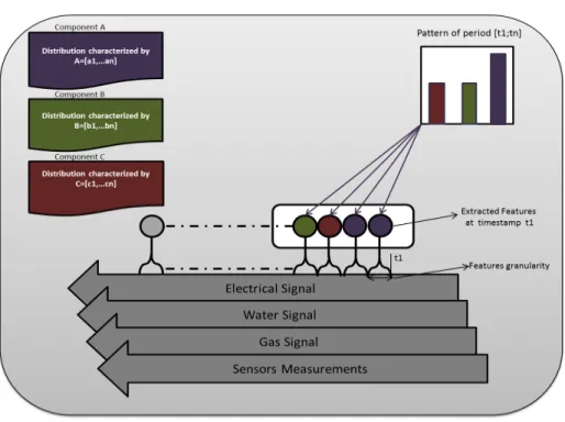
Details on how to compute the local variational parametersφ∗i(λ∗) can be found in [25]. To explain the analogy between LDA and the proposed approach, in Fig. 1, we show an example where three components have been extracted from the utility usage data. Here, the components are equivalent to topics in LDA. Because features extracted by DBN are in discrete space, the components repre-sent categorical distributions over the input features like the LDA’s categorical distributions over words. A pattern is a mixture of components generating the input features over a fixed period of time. In LDA, patterns are associated with documents that can be expressed by mixture of corpus-wide topics. One can clearly notice that this bag-of-words assumption, where temporal dependency in the data is neglected, is a major simplification. However, this simplification leads to methods that are computationally efficient. Such computational efficiency is essential in our case where massive amount of data (around 4 Tb) is used to train the model.
4
Experimental Settings
First, the data is pre-processed in 3 steps: 1) synchronisation of same utility data, 2) alignment of data coming from different utilities and 3) features extraction. Details about the pre-processing steps and data description are given in App. 6. In this section, we focus on the experiments performed on the pre-processed data.
In all experiments, we use the empirical Bayes method to online point es-timate the hyper-parameters from the data. The idea is to maximise the log likelihood of the data with respect to the hyper-parameters. Since the computa-tion of the log likelihood of the data is not tractable, the approximacomputa-tion based on the variational inference algorithm used in Sec. 3.2 is employed. The number of components is fixed toK= 50. We evaluated a range of settings of the learn-ing parameters:κ(learning factor),τ0 (learning delay) and batch sizeBS on a
testing set, where the parametersκandτ0, defined in [33], control the learning
step-size ρj. We used the data collected during the last two weeks (see. Ap. 6) for testing. All experiments are run 30 times.
Fig. 1.Elements of the proposed approach
4.1 Evaluation and Analysis
In order to evaluate LDA, we use the perplexity measure which quantifies the fit of the model to the data. It is defined as the reciprocal geometric mean of the inverse marginal probability of the input in the held-out test set. Since perplexity cannot be computed directly, a lower bound on it is derived in a similar way to the one in [20]. This bound is used as a proxy for the perplexity.
Moreover, to investigate the quality of the results, we study the regularity of the mined patterns by matching them across similar periods of time. For instance, it is expected that similar patterns will emerge in specific hours like breakfast in every morning, watching TV in the evening, etc. Hence, it is inter-esting to understand how such patterns occur as regular events.
Finally, to provide a quantitative evaluation of the algorithm, we propose a mapping method that reveals the specific energy consumed for each pattern. By doing so, we can evaluate numerically the coherence of the extracted patterns by fitting a regression model to the energy consumption over components:
Aw=b (15)
wherewis a vector expressing energy consumption associated with components,
bis a vector representing per-pattern consumption andAis the matrix of the per-pattern components proportions obtained by LDA. This technique will also allow us to numerically check the predicted consumption against the real consumption.
Table 1.Parameter settings Batch size:BS 1 4 8 Learning factor:κ0.7 0.5 0.5 Learning delay:τ0256 64 64 Perplexity 334 333 350
A- Model Fitness: Although online LDA converges for any validκ,τ0andBS,
the quality and speed of the convergence may depend on how the learning param-eters are set. We run online LDA on the training sets forκ∈ {0.5,0.6,0.7,0.8,0.9}, τ0∈ {1,64,256,1024} andBS ∈ {1,4,8}. Table 1 summarises the best settings
of each batch size along with the perplexity obtained on the test set.
The obtained results show that the perplexity for different parameters set-tings are similar. However, the computation complexity increases with the size of the batch. Hence, we set the batch size to 1, where the best learning parameters areκ= 0.7 andτ= 256.
B- Pattern Regularity: Using the optimal parameters’ setting, we examine in the following the regularity of the mined patterns. To do that, we use the data from 11-05-2017 10:10:10 to 25-05-2017 10:10:10 for testing. To study the regularity of the energy consumption behaviour of the residents, we compare the mined patterns across different days of the testing period. These patterns are represented by the proportions of the different components (topics) inferred from the training data. The dissimilarity of the patterns across the two weeks are computed as follows:
dissimilarity(day1, day2) = 1 K∗F F X j=1 K X i=1
|γ(day1)j,i−γ(day2)j,i| (16)
where F = 48 is the number of patterns within the day, K is the number of components, γ(day1)j,i depends on component i of pattern j (see Sec.3.2) of a day from the first week. Table 2 shows the per-day dissimilarity. It can be clearly seen from the table that there are regular patterns across the two weeks. That is, similar energy consumption patterns appear across different days. This similarity is a bit less (i.e., higher dissimilarity) for the weekend where more random activities could take place. Computing the dissimilarity measure between week and weekend days confirms this observation. For instance, the dissimilarity between Monday and Sunday of the first week is equal to 15.25.
This regularity may be caused by regular user lifestyle leading to similar energy consumption behaviour within and across the weeks. Such regularity is violated in the weekend, as more irregular activities could take place. Having shown that there is some regularity in the mined patterns, it is more likely that specific energy consumption can be associated with each component. In the next section, we apply a regression method to map the patterns (e.i., components proportions) to energy consumption. Thus, the parameters of interest are the energy consumption associated with the components. By attaching an energy
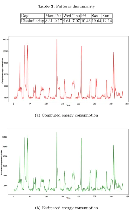
Table 2.Patterns dissimilarity Day Mon Tue Wed Thu Fri Sat Sun Dissimilarity 8.31 9.17 9.61 7.97 10.43 12.64 12.14
(a) Computed energy consumption
(b) Estimated energy consumption
Fig. 2.Evolution of the energy consumption over time
consumption with each component, we can help validate the coherence of the extracted patterns and do forecasting.
C- Energy Mapping: As shown in the previous section, LDA can express the energy consumption patterns by mixing global components summarising data. These global components can be thought of as a base in the space of patterns.
Each component is a distribution over a high-dimensional feature space and understanding what it represents is not easy. Hence, we propose to associate consumption quantities to each component. Such association is motivated by the fact that an energy consumption pattern is normally governed by the usage of different appliances in the house. There should be a strong relation between components and appliances usage. Hence, a relation between components and energy consumption is plausible. Note that the best case scenario occurs if each component is associated with the usage of a specific appliance. Apart from the coherence study, associating energy consumption with each component can be used to forecast the energy consumption. This can be done through pattern forecasting which will be investigated in future work (see Sec. 5). We apply a simple least-square regression method to map patterns to energy consumption, expressed as follows:
min||Aw−b||2 (17)
where wis the per-component energy consumption vector, bis the per-pattern consumption vector andAis the matrix of the per-pattern components’ propor-tions which is computed by LDA. We train the regression model on the week from 18-05-2017 23:45:22 to 25-05-2017 23:45:22 and run the model on the next one from 25-05-2017 23:45:22 to 01-06-2017 23:45:22 . Figure 2 shows the energy consumption (in joules) along with the estimated consumption computed using the learned per-component consumption parameters.
The similarity between the estimated and computed energy consumption demonstrates that the LDA components express distinct usages of energy. Such distinction can be the result of the usage of different appliances likely having dis-tinct energy consumption signatures. Thus, DBN-LDA produces coherent and regular patterns that reflect the energy consumption behaviour and human ac-tivities. Note that it is possible that different patterns (or appliance usages) may have the same energy consumption and that is why both estimated and computed energy consumption in Fig. 2 are not fully the same.
5
Conclusion and Future Work
In this paper, we presented a novel approach to extract patterns of the users’ consumption behaviour from data involving different utilities (e.g, electricity, water and gas) as well as some sensors measurements. DBN-LDA is fully un-supervised and LDA works online which is suitable for dealing with big data. To analyse the performance, we proposed a three-steps evaluation that covers: model fitness, qualitative analysis and quantitative analysis. The experiments show that DBN-LDA is capable of extracting regular and coherent patterns that highlight energy consumption over time. In the future, we foresee three direc-tions for research to improve the obtained results and provide more features: (i) developing online dynamic latent Dirichlet allocation (DLDA) to consider the temporal dependency in the data leading to better results and allowing forecast-ing, (ii) develop more scalable LDA by applying asynchronous distributed LDA which can be derived from [35] instead of SVI and (iii) involving active learning strategy to query users about ambiguous or unknown activities in order to guide the learning process when needed [36, 37].
Acknowledgment
This work was supported by the Energy Technology Institute (UK) as part of the project: High Frequency Appliance Disaggregation Analysis (HFADA). A. Bouchachia was supported by the European Commission under the Horizon 2020 Grant 687691 related to the project:PROTEUS: Scalable Online Machine Learning for Predictive Analytics and Real-Time Interactive Visualization.
References
1. A. Bulling, U. Blanke, and B. Schiele, “A tutorial on human activity recognition using body-worn inertial sensors,”ACM Computing Surveys (CSUR), vol. 46, no. 3, p. 33, 2014.
2. R. Poppe, “A survey on vision-based human action recognition,”Image and vision computing, vol. 28, no. 6, pp. 976–990, 2010.
3. S. Wang and G. Zhou, “A review on radio based activity recognition,” Digital Communications and Networks, vol. 1, no. 1, pp. 20–29, 2015.
4. G. W. Hart, “Nonintrusive appliance load monitoring,”Proceedings of the IEEE, vol. 80, no. 12, pp. 1870–1891, 1992.
5. M. Zeifman and K. Roth, “Nonintrusive appliance load monitoring: Review and outlook,”IEEE transactions on Consumer Electronics, vol. 57, no. 1, 2011. 6. A. Zoha, A. Gluhak, M. A. Imran, and S. Rajasegarar, “Non-intrusive load
mon-itoring approaches for disaggregated energy sensing: A survey,” Sensors, vol. 12, no. 12, pp. 16 838–16 866, 2012.
7. J. Liang, S. K. Ng, G. Kendall, and J. W. Cheng, “Load signature studypart i: Basic concept, structure, and methodology,”IEEE transactions on power Delivery, vol. 25, no. 2, pp. 551–560, 2010.
8. J. Z. Kolter, S. Batra, and A. Y. Ng, “Energy disaggregation via discriminative sparse coding,” inAdvances in Neural Information Processing Systems, 2010, pp. 1153–1161.
9. D. Srinivasan, W. Ng, and A. Liew, “Neural-network-based signature recognition for harmonic source identification,”IEEE Transactions on Power Delivery, vol. 21, no. 1, pp. 398–405, 2006.
10. M. Berges, E. Goldman, H. S. Matthews, and L. Soibelman, “Learning systems for electric consumption of buildings,” inComputing in Civil Engineering (2009), 2009, pp. 1–10.
11. A. G. Ruzzelli, C. Nicolas, A. Schoofs, and G. M. O’Hare, “Real-time recognition and profiling of appliances through a single electricity sensor,” in Sensor Mesh and Ad Hoc Communications and Networks (SECON), 2010 7th Annual IEEE Communications Society Conference on. IEEE, 2010, pp. 1–9.
12. J. Kelly and W. Knottenbelt, “Neural nilm: Deep neural networks applied to en-ergy disaggregation,” in Proceedings of the 2nd ACM International Conference on Embedded Systems for Energy-Efficient Built Environments. ACM, 2015, pp. 55–64.
13. Y.-X. Lai, C.-F. Lai, Y.-M. Huang, and H.-C. Chao, “Multi-appliance recognition system with hybrid SVM/GMM classifier in ubiquitous smart home,”Information Sciences, vol. 230, pp. 39–55, 2013.
14. R. Bonfigli, S. Squartini, M. Fagiani, and F. Piazza, “Unsupervised algorithms for non-intrusive load monitoring: An up-to-date overview,” in Environment and Electrical Engineering (EEEIC), 2015 IEEE 15th International Conference on. IEEE, 2015, pp. 1175–1180.
15. R. Salakhutdinov, J. B. Tenenbaum, and A. Torralba, “Learning with hierarchical-deep models,” IEEE transactions on pattern analysis and machine intelligence, vol. 35, no. 8, pp. 1958–1971, 2013.
16. Y. LeCun, Y. Bengio, and G. Hinton, “Deep learning,”nature, vol. 521, no. 7553, p. 436, 2015.
17. L. Deng, “A tutorial survey of architectures, algorithms, and applications for deep learning,” APSIPA Transactions on Signal and Information Processing, vol. 3, 2014.
18. Y. Bengioet al., “Learning deep architectures for AI,”Foundations and trendsR in Machine Learning, vol. 2, no. 1, pp. 1–127, 2009.
19. G. E. Hinton, S. Osindero, and Y.-W. Teh, “A fast learning algorithm for deep belief nets,”Neural computation, vol. 18, no. 7, pp. 1527–1554, 2006.
20. D. M. Blei, A. Y. Ng, and M. I. Jordan, “Latent dirichlet allocation,”Journal of machine Learning research, vol. 3, no. Jan, pp. 993–1022, 2003.
21. C. Fischer, “Feedback on household electricity consumption: a tool for saving en-ergy?”Energy efficiency, vol. 1, no. 1, pp. 79–104, 2008.
22. J. Kelly and W. Knottenbelt, “The UK-DALE dataset, domestic appliance-level electricity demand and whole-house demand from five uk homes,”Scientific data, vol. 2, p. 150007, 2015.
23. A. Filip, “Blued: A fully labeled public dataset for event-based non-intrusive load monitoring research,” in 2nd Workshop on Data Mining Applications in Sustain-ability (SustKDD), 2011, p. 2012.
24. J. Z. Kolter and M. J. Johnson, “REDD: A Public Data Set for Energy Disag-gregation Research,” in Workshop on Data Mining Applications in Sustainability (SIGKDD), San Diego, CA, vol. 25, no. Citeseer, 2011, pp. 59–62.
25. M. D. Hoffman, D. M. Blei, C. Wang, and J. Paisley, “Stochastic variational infer-ence,”The Journal of Machine Learning Research, vol. 14, no. 1, pp. 1303–1347, 2013.
26. S. Makonin, F. Popowich, L. Bartram, B. Gill, and I. V. Bajic, “Ampds: A public dataset for load disaggregation and eco-feedback research,” inElectrical Power & Energy Conference (EPEC), 2013 IEEE. IEEE, 2013, pp. 1–6.
27. S. Makonin, B. Ellert, I. V. Baji´c, and F. Popowich, “Electricity, water, and natural gas consumption of a residential house in canada from 2012 to 2014,”Scientific data, vol. 3, 2016.
28. H. Kim, M. Marwah, M. Arlitt, G. Lyon, and J. Han, “Unsupervised disaggre-gation of low frequency power measurements,” in Proceedings of the 2011 SIAM International Conference on Data Mining. SIAM, 2011, pp. 747–758.
29. J. Z. Kolter and T. Jaakkola, “Approximate inference in additive factorial hmms with application to energy disaggregation,” inArtificial Intelligence and Statistics, 2012, pp. 1472–1482.
30. M. J. Johnson and A. S. Willsky, “Bayesian nonparametric hidden semi-markov models,” Journal of Machine Learning Research, vol. 14, no. Feb, pp. 673–701, 2013.
31. M. Wytock and J. Z. Kolter, “Contextually Supervised Source Separation with Application to Energy Disaggregation.” inAAAI, 2014, pp. 486–492.
32. M. Saad and B. Abdelhamid, “Online gaussian LDA for unsupervised pattern mining from utility usage data,”submitted to ECML-PKDD, 2018.
33. M. Hoffman, F. R. Bach, and D. M. Blei, “Online learning for latent dirichlet allocation,” inadvances in neural information processing systems, 2010, pp. 856– 864.
34. H. Robbins and S. Monro, “A stochastic approximation method,”The annals of mathematical statistics, pp. 400–407, 1951.
35. S. Mohamad, A. Bouchachia, and M. Sayed-Mouchaweh, “Asynchronous stochastic variational inference,”arXiv preprint arXiv:1801.04289, 2018.
36. S. Mohamad, M. Sayed-Mouchaweh, and A. Bouchachia, “Active learning for clas-sifying data streams with unknown number of classes,”Neural Networks, vol. 98, pp. 1–15, 2018.
37. S. Mohamad, A. Bouchachia, and M. Sayed-Mouchaweh, “A bi-criteria active learn-ing algorithm for dynamic data streams,”IEEE Transactions on Neural Networks and Learning Systems, 2016.
6
Appendix
In this section, we will first introduce the experimental data, LDA will be tested on along with details about the data pre-processing stages.
6.1 Datasets
The real-world multi-source utility usage data used here is provided by ETI1.
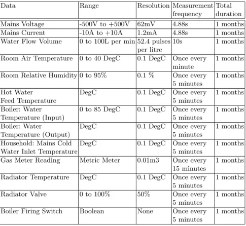
The data includes electricity signals (voltage and current signals) sampled at high sampling rate around 205 kHz, water and gas consumption sampled at low sampling rate. The data also contains other sensors measurements collected from the Home Energy Monitoring System (HEMS). In this study we will use 4Tb of utility usage data collected from one house over one month. This data has been recorded into three different formats. Water data is stored in text files with sampling rate of 10 seconds and is synchronised to Network Time Protocol (NTP) approximately once per month. Electricity data is stored in wave files with sampling rate of 4.88 s and is synchronised to NTP every 28min 28sec. HEMS data is stored in a Mongo database with sampling rates differing according to the type of the data and sensors generating it (see Tab. 3).
Data Pre-processing In order to exploit raw utility data by LDA, a number of pre-processing steps are required. We read the data from the different sources, synchronise its time-stamps to NTP time-stamps, extract features and align the data samples to one time-stamp by measurement. For water data, the PC clock time-stamps of samples within each month are synchronised to NTP time-stamp. The synchronisation is done as follows:
timestampN T P(i) =timestampsclock(i) +i T otal T ime Shif t
N umber of Samples (18) In this equation, we assume that the total shift (between NTP and PC clock) can be distributed over the samples in one month. Similarly, Electricity data samples’ time-stamps are synchronised to NTP time-stamps. The shift is distributed over 28 minutes and 28 seconds.
timestampN T P(i) =timestampsclock(i) +i T otal T ime Shif t
N umber of Samples (19) The time-stamps of HEMS data were collected using NTP and so no synchro-nisation is required. Having all data samples synchronised to the same reference (NTP), we align the samples to the same time-stamps. The alignment strategy is shown in Fig. 3 where the union of all aligned data samples is stored in one matrix. Each row of this matrix includes a time-stamp and the corresponding values of the sensors. If for some sensors, there are no measurements taken at the time-stamp, the values measured at the previous time stamp are taken. The
1
Table 3.Characteristics of the data
Data Range Resolution Measurement Total
frequency duration Mains Voltage -500V to +500V 62mV 4.88s 1 months
Mains Current -10A to +10A 1.2mA 4.88s 1 months
Water Flow Volume 0 to 100L per min 52.4 pulses 10s 1 months per litre
Room Air Temperature 0 to 40 DegC 0.1 DegC Once every 1 months minute
Room Relative Humidity 0 to 95% 0.1 % Once every 1 months 5 minutes
Hot Water DegC 0.1 DegC Once every 1 months
Feed Temperature 5 minutes
Boiler: Water 0 to 85 DegC 0.1 DegC Once every 1 months
Temperature (Input) 5 minutes
Boiler: Water DegC 0.1 DegC Once every 1 months
Temperature (Output) 5 minutes
Household: Mains Cold DegC 0.1 DegC Once every 1 months
Water Inlet Temperature 5 minutes
Gas Meter Reading Metric Meter 0.01m3 Once every 1 months 15 minutes
Radiator Temperature DegC 0.1 DegC Once every 1 months 5 minutes
Radiator Valve 0 to 100% 50% Once every 1 months 5 minutes
Boiler Firing Switch Boolean None Once every 1 months 5 minutes
Fig. 3.Alignment of the data
aligned data samples are the input of the feature extraction model (Deep Belief Network). Pushed by the complexity of the mining task and motivated by the informativeness and simplicity of the water and sensors data, at this stage, we apply DBN only on the electricity data over time windows of 1 second.
The employed DBN2consists of three Restricted Boltzmann Machine layers
where the first layer reduces the input dimension from 204911 (1 second granu-larity) to 700. The second and third layers’ outputs dimensions are 200 and 100 respectively. Note that the first layer’s inputs are from continuous space while the rest is categorical data. The rest parameters are left to the default setting. The last layer’s outputs are aligned and concatenated with the other utility and sensors discretised data.
2