Bucket Hashing and its Application to
Fast Message Authentication
Phillip Rogaway
Department of Computer Science, University of California, Davis, CA 95616. e-mail: [email protected]
October 13, 1997
Earlier version appears inAdvances in Cryptology – CRYPTO ’95. This is the full paper.
Abstract. We introduce a new technique for constructing a family of universal hash functions. At its center is a simple metaphor: to hash a string x, cast each of its words into a small number ofbuckets; xor the contents of each bucket; then collect up all the buckets’ contents. Used in the context of Wegman–Carter authentication, this style of hash function provides a fast approach for software message authentication.
Key words: Cryptography, Hashing, Message authentication codes, Universal Hashing.
1
Introduction
Message authentication. Message authentication is one of the most common cryptographic
aims. The setting is that two parties, a signer S and verifier V, share a (short, random, secret) key, k. WhenS wants to send V a message, x, S computes for it a message authentication code
(MAC),σ←MACk(x), andS sends V the pair (x, σ). On receipt of (x, σ), verifierV checks that MACVk(x, σ) = 1.
To describe the security of a message authentication scheme, an adversary E is given an oracle for MACk(·). The adversary is declared successful if she outputs an (x∗, σ∗) such that MACVk(x∗, σ∗) = 1 but x∗ was never asked of the MACk(·) oracle. For a scheme to be “good,” reasonable adversaries should rarely succeed.
Software-efficient MACs. In the current computing environment it is often necessary to
compute MACs frequently and over strings which are commonly hundreds to thousands of bytes long. Despite this, there will usually be no special-purpose hardware to help out: MAC generation and verification will need to be done in software on a conventional workstation or personal computer. So to reduce the impact of message authentication on the machine’s overall performance, and to facilitate more pervasive use of message authentication, we need to develop faster techniques. This paper provides one such technique.
Two approaches to message authentication. The fastest software MACs in common use
today are exemplified by MACk(x) =h(kxk), with h a (software-efficient) cryptographic hash function, such as h =MD5 [22]. Such methods are described in [30]. The algorithm HMAC [3]
represents the most refined algorithm in this direction. Schemes like these might seem to be about as software-efficient as one might realistically hope for: after all, we are computing one of the fastest types of cryptographic primitives over a string nearly identical in length to that which we want to authenticate. But it is well-known that this reasoning is specious: in particular, Wegman and Carter [32] showed back in 1981 that we do not have to “cryptographically” transform the entire stringx.
In the Wegman–Carter approach communicating partiesS and V share a secret keyk= (h, P) which specifies both an infinite random stringP and a functionh drawn randomly from a strongly universal2 family of hash functions H. (Recall that H is strongly universal2 if for all x = x, the random variable h(x) h(x), for h ∈ H, is uniformly distributed.) To authenticate a message x, the sender transmitsh(x) xor-ed with the next piece of the pad P. The thing to notice is that xis transformed first by a non-cryptographic operation (universal hashing) and only then is it subjected to a cryptographic operation (encryption), now applied to a much shorter string.
A standard cryptographic technique —the use of a pseudorandom function family,F— allowsS
and V to use a short stringain lieu of the infinite string P. SignerS now MACs theith message,
xi, with MAC(h,a)(xi) = (i, Fa(i)⊕h(xi)).
As it turns out, to make a good MAC it is enough to construct something weaker than a strongly universal2family. Carter and Wegman [10] also introduced the notion of an almost universal2family,
H. This must satisfy the weaker condition that Prh∈H[h(x) = h(x)] is small for all x = x. As observed by Stinson [27], an almost universal2 family can easily be turned into an almost strongly universal2 family by composing the almost universal2 family with an almost strongly universal2 one. In computingh2(h1(x)), where h1 is drawn from an almost universal2 family andh2 is drawn from a strongly universal2 one, the bulk of the time will typically be spent in computing h1(x), sincex may be a long string buth1(x) will be a short string, and soh2 won’t have much work left to do. Thus the problem of finding a fast-to-compute MAC has effectively been reduced to finding a family of almost universal2 hash functions whose members are fast to compute.
Bucket hashing. This paper provides a new almost universal2 family of hash functions. We call
our hash familybucket hashing. It is distinguished by its member functions being extremely fast to compute—as few as 6 elementary machine instructions per word (independent of word size) for the version of bucket hashing we concentrate on in this paper. Putting such a family of hash functions to work in the framework described above will give rise to an efficient software MAC.
A bucket hash MAC will involve significant overhead beyond the time which is spent bucket hashing. For one thing, the output of bucket hashing is too long to use directly; it will need to be composed with an additional layer of hashing. All the same, one can compare the instruction count mentioned above to that of MD5, which uses ≈36 instructions per 32-bit word [7], and see that there is potential for substantial efficiency gains even if the true cost of using bucket hashing substantially exceeds 6 instructions/word.
A bucket hash MAC has advantages in addition to speed. Bucket hashing is a linear function —it is a special case of matrix multiplication over GF(2)— and this linearity yields many pleasant characteristics for a bucket hash MAC. In particular, bucket hashing is parallelizable, since each word of the hash is just the xor of certain words of the message. Bucket hashing is incremental in the sense of [4] with respect to bothappendandsubstituteoperations. Finally, the only processor instructions a bucket hash needs are word-alignedload,store, and xor; thus a bucket hash MAC is essentially endian-indifferent.
In a bucket hash MAC —indeed in any Wegman-Carter MAC— one is afforded the luxury of conservative (slow) cryptography even in a MAC whose software speed has been aggressively
optimized. This is because one arranges that the time complexity for the MAC is dominated by the non-cryptographic work.
One might worry that the linearity or simple character of bucket hashing might give rise to some “weakness” in a MAC which exploits it. But it does not. A bucket hash MAC, like any MAC which follows the Wegman–Carter paradigm, enjoys the assurance advantages of provable security. Moreover, this provable security is achieved under extremely “tight” reductions, so that an adversary who can successfully break the MAC can break the underlying cryptographic primitive (the pseudorandom function F) with essentially identical efficiency.
Previous work. The general theory of unconditional authentication was developed by Simmons;
see [26] for a survey. As we have already explained, the universal-hash-and-then-encrypt paradigm is due to Wegman and Carter [32]. The idea springs from their highly influential [10].
In Wegman–Carter authentication the size of the hash family corresponds to the number of bits of shared key—one reason to find smaller families of universal hash functions than those of [10, 32]. Siegel (for other reasons) [25] constructs families of fast-to-compute hash functions which use few bits of randomness and have small description size. Stinson finds small hash families in [27], and also gives general results on the construction of universal hash functions. We exploit some of these ideas here. Subsequent improvements (rooted in coding theory) came from Bierbrauer, Johansson, Kabatianskii and Smeets [6], and Gemmell and Naor [12].
The above work concentrates on universal hash families and unconditionally-secure authenti-cation. Brassard [9] first connects the Wegman–Carter approach to the complexity-theoretic case. The complexity-theoretic notion for a secure MAC is a straightforward adaptation of the definition of a digital signature due to Goldwasser, Micali and Rivest [14]. Their notion of an adaptive cho-sen message attack is equally at home for defining an unconditionally-secure MAC. Thus we view work like ours as making statements about unconditionally-secure authentication which give rise to corresponding statements and concrete schemes in the complexity-theoretic tradition. To make this translation we regard a finite pseudorandom function (PRF) as the most appropriate tool. Bellare, Kilian and Rogaway [5] were the first to formalize such objects, investigate their usage in the construction of efficient MACs, and suggest them as a desirable starting point for practical, provably-good constructions. Finite PRFs are a refinement of the PRF notion of Goldreich, Gold-wasser and Micali [13] to take account of the fixed lengths of inputs and outputs in the efficient primitives of cryptographic practice.
Zobrist [33] gives a hashing technique which predates [10] and essentially coincides with one method from [10]. Arnold and Coppersmith [2] give an interesting hashing technique which allows one to map a set of keys ki into a set of corresponding values vi using a table only slightly bigger thanivi. The proof of our main technical result is somewhat reminiscent of their analysis.
Lai, Rueppel and Woolven [19], Taylor [28], and Krawczyk [18] have all been interested in computationally efficient MACs. The last two works basically follow the Wegman–Carter paradigm. In particular, Krawczyk obtains efficient message authentication codes from hash families which resemble traditional cyclic redundancy codes (CRCs), and matrix multiplication using Toeplitz matrices. Though originally intended for hardware, these techniques are fast in software, too. We recall Krawczyk’s CRC-like hash in Section 2.
An earlier version of this paper appeared as [23].
Subsequent work. Shoup [24] has carried out implementations and analysis of hash function
families akin to polynomial evaluation. Such hash functions make good candidates for “second level hashing” when a speed-optimized hash function is applied to a long string. The techniques are also
fast enough to be gainfully employed all by themselves.
Halevi and Krawczyk describe a family of hash functions, MMH, which achieves extremely impressive software speeds on some modern platforms [15]. To achieve such performance one needs the underlying hardware to be able to quickly multiply two 32-bit integers to form a 64-bit product. Johansson investigates how to reduce the size of the key for bucket hashing, which, in the current paper, is quite enormous [16].
Organization. We continue in Section 2 by reviewing the definition and basic properties of
universal hash families. Sections 3 and 4 give our main result. In the former we formally define our family of hash functions, B; we state a theorem which upper bounds the collision probability of B; and we discuss the efficiency of computing functions drawn fromB. In the latter we prove our main theorem, relegating one lemma to Appendix A. Section 5 reviews the Wegman-Carter approach for making a MAC out of a family of universal hash functions, while Section 6 gives a concrete example of this and discusses some of the difficulties involved in constructing a good MAC using bucket hashing. Section 7 considers some extensions and directions for our work.
2
Preliminaries
This section provides background drawn from Carter and Wegman [10, 32], Stinson [27], and Krawczyk [18]. Proofs are omitted.
A family of hash functions is a finite multisetH of string-valued functions, each h∈ H having the same nonempty domain A⊆ {0,1}∗ and range B ⊆ {0,1}b, for some constantb.
Definition 1 [10] A family of hash functions H = {h : A → {0,1}b} is -almost universal2, written -AU2, if for all distinctx, x ∈A, Pr
h∈H
h(x) =h(x)≤. The family of hash functionsH is-almost XOR universal2, written-AXU2, if for all distinctx, x∈A, and for allc∈ {0,1}b,
Pr h∈H
h(x)⊕h(x) =c≤.
The value of= maxx=x{Prh[h(x) =h(x)]}is called thecollision probability. For us, the principle measures of the worth of an AU2 hash family are how small is its collision probability and how fast can one compute its functions.
To make a fast MAC one may wish to “glue together” various universal hash families. The following are the basic methods for doing this.
First we need a way to make the domain of a hash family bigger. LetH={h:{0,1}a→ {0,1}b}. ByHm ={h:{0,1}am → {0,1}bm}we denote the family of hash functions whose elements are the same as inH but whereh(x1x2· · ·xm), for|xi|=a, is defined byh(x1)h(x2) · · · h(xm). Proposition 2 [27]If His -AU2 thenHm is-AU2.
Sometimes one needs a way to make the collision probability smaller. LetH1={h:A→ {0,1}b1} and H2={h:A→ {0,1}b2}be families of hash functions. ByH1&H2 ={h:A→ {0,1}b1+b2}we mean the family of hash functions whose elements are pairs of functions (h1, h2) ∈ H1 × H2 and where (h1, h2)(x) is defined as h1(x)h2(x).
Next is a way to make the image of a hash function shorter. LetH1 ={h:{0,1}a→ {0,1}b} and
H2 = {h : {0,1}b → {0,1}c} be families of hash functions. Then by H2 ◦ H1 = {h : {0,1}a →
{0,1}c}we mean the family of hash function whose elements are pairs of functions (h1, h2)∈ H1×H2 and where (h1, h2)(x) is defined as h2(h1(x)).
Proposition 4 [27]If H1 is 1-AU2 andH2 is 2-AU2 then H2◦ H1 is(1+2)-AU2.
Composition can also be used to turn an AU2 family H1 whose members hash A to B, and an AXU2 familyH2 whose members hash B toC, into an AXU2 familyH2◦ H1 whose members hash
A to C. If B ={0,1}b for some small b, and elements of H2 are fast to compute on this domain, we have effectively “promoted”H1 from being AU2 to AXU2 at little cost.
Proposition 5 [27] Suppose H1 ={h :A→ B} is 1-AU2, and H2 ={h :B →C} is2-AXU2. Then H2◦ H1={h:A→C} is(1+2)-AXU2.
We end this section with a sample construction for a software-efficient AXU2 hash family, this one due to Krawczyk [18]. Let n, ≥ 1 be numbers and let m ∈ {0,1}n be the string we wish to hash. We can view m as a polynomial m(x) over GF(2) of degree n−1 (or less) by viewing the bits of m as the coefficients of xn−1, . . . , x2, x,1. We then define a family of hash functions
K[n, ] = {h : {0,1}n → {0,1}} as follows. A random hash function h ∈ K is described by a random irreducible polynomial h over GF(2) of degree . To hash m using h we compute the degree −1 (or less) polynomialm(x)·x modh(x). Viewing the coefficients of this polynomial as a string of length gives us the hash function h evaluated atm.
Theorem 6 [18] K[n, ]is n2+−1-AXU2.
The efficiency with which hash functions h ∈ K can be computed has been studied by Shoup [24] (who also looked at related hash families). These functions are fast to compute— about 6 in-structions/byte on a 32-bit machine, assuming = 64, and ignoring the time to “preprocess” the functionh. Still, for sufficiently long messages, it will be faster to use the bucket hashing technique from the following section.
We comment that there are many other well-known techniques for universal hashing, such as the linear congruential hash (modulo a prime) [10], the shift register hash [31], or the Toeplitz matrix hash [18].
3
Bucket Hashing
Let X = X1. . . Xn be a string, partitioned into n words. To hash X using bucket hashing we will scatter the words of X into N “buckets,” then XOR the contents of each bucket, and then concatenate the bucket contents.
Some ways of scattering the words of X work out better than others. In this paper we analyze a particular bucket hashing scheme, which we denote byB. The scheme will depend on parameters
3.1 Defining the bucket hash family B
Fix a word size w ≥ 1 and parameters n ≥ 1 and N ≥ 3. We will be hashing from domain
D={0,1}wn to rangeR ={0,1}wN. As a typical example, take w= 32, n= 1024, andN = 140. If we want to be explicit, such a family would be denoted B[32,1024,140]. For the scheme we describe to make sense we require that N3≥n.
Each hash function h∈ B is specified by a length-n list of cardinality-3 subsets of {1, . . . , N}. We denote this list by h=h1· · ·hn. The three elements of hi are written hi ={hi1, hi2, hi3}.
Choosing a random h from B[w, n, N] means choosing a random length-n list of three-element subsets of{1, . . . , N}subject to the constraint that no two of these sets are the same. That is, we insist thathi=hj for all i=j.
Leth∈ Band letX=X1· · ·Xnbe the string we want to hash, where each|Xi|=w. Thenh(X) is defined by the following algorithm. First, for each j∈ {1, . . . , N}, initializeYj to 0w. Then, for each i∈ {1, . . . , n}and k∈hi, replaceYk by Yk⊕Xi. When done, seth(X) =Y1Y2 · · · YN.
In pseudocode we have: for j ←1 to N do Yj ←0w for i←1 to n do Yhi1 ←Yhi1 ⊕Xi Yhi2 ←Yhi2 ⊕Xi Yhi3 ←Yhi3 ⊕Xi return Y1 Y2 · · · YN
The computation of ah(X) can be envisioned as follows. We haveN buckets, each initially empty. The first word of X is thrown into the three buckets specified by h1. The second word of X is thrown into the three buckets specified byh2. And so on, with the last word ofXbeing thrown into the three buckets specified byhn. Our N buckets now contain a total of 3nwords. Compute the xor of the words in each of the buckets (with the xor of no words being defined as the zero-word). The hash of X,h(X), is the concatenation of the final contents of theN buckets.
3.2 Collision probability of the bucket hash family B
The collision probability for B[w, n, N]. is the maximum, over all distinct x, x ∈ {0,1}nw, of the probability thath(x) =h(x). Our main theorem gives an upper bound on the collision probability of B. The bound is about 3312N−6. In other words,B[w, n, N] is-AU2 for≈3312N−6.
Theorem 7 [Main result] Assume w ≥ 1, N ≥ 32 and n ≤ N3/12. Let be the collision probability for B[w, n, N]. Then ≤B(N), where B(N) =λ(N)β(N), for λ(N) = 1/(1−6/N3)
and
β(N) = 720(N−3)(N−4)(N−5)+1944(N−3)(N−4)
2+648(N−2)(N−3)2 N3(N−1)3(N−2)3 . The proof of Theorem 7 is given in Section 4.
Plot of B(N). In Figure 1 we plotB(N) againstN. Consulting the graph we see, for example,
that if you hash a string down to 140 words the collision probability is about 2−31.
Comments. In the applications of bucket hashing to message authentication one typically wants
collision probability requires a fairly large value of N. Since N is the length of our hashed string (in words), large values ofN are undesirable and typically require additional layers of hashing. An example of this will be illustrated in Section 5.
Note that our bound shows no dependency onw orn(though there is the technical restriction that n ≤ N3/12). Indeed it is easy to see (and the proof of Theorem 7 will show) that the collision probability does not depend on w. In fact, it is a consequence of the proof that, when 4≤n≤N3/12, the collision probability does not depend onn, either.
Observe that λ(N) = N/(N −36), where N = N(N−1)(N−2). By our assumption that
N ≥32 we have that 1≤λ(N)≤1.002. So the multiplication byλ(N) can effectively be ignored;
B(N)≈β(N).
We believe that it is possible to relax the restrictionn≤N3/12 all the way ton <N3. However, doing this would add considerable complexity to the proof, yet have relatively little practical value, since the number of buckets, N, needs to quite large in order to obtain what would usually be regarded as a suitably small collision probability.
Explanation. Here is a bit of intuition for what is going on. Suppose an adversary wants to
find a pair of distinct messages x, x ∈ {0,1}wn which are most likely to collide under a function fromB. What two messages should she choose? In the proof of Theorem 7 we recast this question into the following one. An adversary will throw t triples of balls into N buckets. Each of the 3t
balls will land in a random bucket, except for the following constraints: three distinct buckets are selected for the three balls of each toss; and no tosses will land in identical triples of buckets. The adversary’s goal is the following: make every bucket end up with an even number of balls in it. All the adversary can do is choose how many triples of balls, t, she will disperse. The question we must answer is: what choice of t, where 1 ≤t ≤ n, will maximize the adversary’s chance to win this game?
It is not hard to guess the right answer to this question: four. Here is an explanation. If the adversary tosses just one triple of balls into the buckets she can’t possibly win: 3 buckets are guaranteed to have an odd number of balls. If she throws outtwotriples of balls she again can not win, thanks to the constraint that no two triples of balls land in identical triples of buckets. If she throws out three triples of balls she again can not win because 9 balls can’t be distributed into buckets in such a way that every bucket has an even number of balls. If the adversary throws out four triples of balls then, finally, she has a chance to win. This seems like it ought to be the best thing for the adversary to do, because it would seem to become increasingly unlikely to get every
bucket to have an even number of balls when more balls get tossed into the N buckets. Though this intuition is a long way from being formal, four triples of balls does turn out to be the right answer. Translating back into the adversary’s original goal, the adversary can do no better than to choose messages X and X which differ by exactly 4 words: for X these words are, say, 0w, while forX these words are, say, 1w.
3.3 The efficiency of the bucket hash family B
Instruction counts. To get a feel for the efficiency of bucket hashing, let us do some approximate
instruction counts for computing a function h ∈ B. Though instruction counting is an extremely crude predictor of speed, an analysis like this is still a good implementation-independent way to get some feel for our method’s potential efficiency.
To construct a good MAC we will probably want a collision probability of ≈ 2−30 (perhaps less) and so, in view of Figure 1, we will be using a reasonably large value ofN, sayN ≥120. Thus
2**-35 2**-34 2**-33 2**-32 2**-31 2**-30 2**-29 2**-28 2**-27 2**-26 2**-25 2**-24 2**-23 2**-22 2**-21 2**-20 40 60 80 100 120 140 160 180 200
Upper bound on collision probablity, B(N)
Number of buckets, N
Figure 1: A graphical representation of Theorem 7. We plot of N verses, B(N), our bound on the collision probability of B[w, n, N].
we will be needing more buckets than can be accommodated by a typical machine’s register set. There are then two natural strategies to hash the string X =X1. . . Xn, where eachXi is a word of the machine’s basic word size:
• Method-1 (Process words X1, . . . , Xn). We can read each Xi from memory (in sequence) and then, three times: (1) load from memory the value Yj of the appropriate bucket j; (2) compute Xi⊕ Yj; (3) store this back into memory, modifyingYj. Total instruction count is 10 instructions per word (4 reads, 3 writes, 3 xors).
• Method-2 (Fill buckets Y1, . . . , YN). We can xor together all words that should wind up in bucket 1; then xor all words that go into bucket 2; and so forth, for each of the N buckets. We will need a total of 3nreads into X1, . . . , Xn, plus 3n−N xor operations (assuming each bucket contains at least one word). Depending on what we want done with the hash, we may need anotherN writes to put the hash value back into memory. So the total instruction count is about 6 instructions per word.
Achieving the stated instruction counts requires the use of self-modifying code (“sm-code”); in effect, we implicitly assumed that the representation ofh∈ Bis the piece of executable code which computes h. In implementation, this can be tricky. If we don’t want to use self-modifying code (“sm-code”) we will need to load from memory the bucket locations (Method-1) or word location (Method-2). This would add 3 loads per word. For Method 2, sm-code would further increase the instruction count because of the overhead needed to control the looping: it is h-dependent how many words will fall into a given bucket, so this will have to be read from memory, and loop-unrolling may be difficult. Assuming an additional one instruction per word to account for this work, we have the following approximate instruction counts:
implementation ≈ instrs/wd
Method-1, sm-code 10
Method-1, sm-code 13
Method-2, sm-code 6
Method-2, sm-code 10
The sm-code uses a table to specifyh. Assume a machine with a word size of 32 bit. For Method-1 the needed table would typically be 3nor 12nbytes long (depending on whether one packs bucket indices into bytes or words). For Method-2 that table would typically be be 6n or 12n bytes long (depending on whether one packs word indices into double-bytes or words), plus an additional N
or 4N bytes long (depending on whether one packs counter-limits into bytes or words). To get a fast implementation, tables need to fit into cache. Note that there is better locality of reference for Method-1 than Method-2, and this can have a substantial efficiency impact when actually coded.
Implementation. A variety of bucket hashing schemes have been implemented (that is, B and
methods similar to B). The observed performance of these implementations varies enormously ac-cording to the particular scheme, the parameters nand N, and the implementation. As a couple points of reference: on a typical 32-bit RISC machine (an SGI with a 150 MHz IP22 processor, 16 KByte data cache, 16 KBytes instruction cache) the most straightforward Method-1/sm imple-mentation ran at 340 Mb/s to hash 1024 words to 140, while a Method-2/sm impleimple-mentation of a bucket hash family based on theC[10,6] graph (see Section 7) ran at 1160 Mb/s to hash 909 words to 182.
Rough comparisons. Shoup estimates a cost of about 24 instructions/word (6 instructions per
byte) for computing a hash functionh∈ K[n,64], whereKis described in Section 2 [24]. Bosselaers, Govaerts and Vandewalle have implemented MD5 at a cost of 36 instructions/word on a Pentium [7] (they obtain a good degree of overlapping instruction-issue, too). In recent work, Halevi and Krawczyk estimate a cost of about 7.5 instructions per word (assuming architectural support for multiplying two 32-bit words to yield a 64-bit product) for their MMH technique [15]. We emphasize that trying to compare such numbers hides many significant factors, including length of hash output (worst for bucket hashing), table sizes and caching issues, and the degree of available parallelism. We have not studied these tradeoffs in detail and do not know if bucket hashing will eventually “win out” in the choice of hash techniques for making a practical MAC.
4
Proof of the Main Theorem
In this section we prove Theorem 7. Throughout this section fix values of nand N satisfying the conditions of the theorem.
Our first two claims show how to simplify the setting.
One can assume a word length of w= 1. First we argue that, without loss of generality, we
can assume that the word length forB[w, n, N] isw= 1. Intuitively, this follows from the “bitwise” character of bucket hashing: when we hash X1· · ·Xn down to Y1· · ·YN, where |Xi|= |Yj|= w, the-th bit ofYi depends only onX1[], . . . , Xn[]. For this reason, no advantage can be gained by trying to exploit long words.
Claim 8 max X,X∈{0,1}nw X=X Pr H∈B[w,n,N] H(X) =H(X)= max x,x∈{0,1}n x=x Pr h∈B[1,n,N] h(x) =h(x).
Proof: Let X, X ∈ {0,1}wn be distinct strings which maximize PrH[H(X) = H(X)]. Since
X =X there must be some bit position 1≤≤wsuch that the n-bit stringsx=X1[]· · ·Xn[] and x = X1[]· · ·Xn[] are distinct. Now notice that we can treat any H ∈ B[w, n, N] as a hash function h = H from B[1, n, N], and conversely, because the description of a bucket hash hash function (a sequence of triples of indices) is insensitive to the word length w. Furthermore,
H(X) =H(X) implies that h(x) =h(x), and so PrH[H(X) =H(X)]≤Prh[h(x) =h(x)] . We conclude that maxX,XPrH[H(X) =H(X)]≤maxx,xPrh[h(x) =h(x)].
For the opposite inequality, let x, x ∈ {0,1}n be distinct strings which maximize Prh[h(x) =
h(x)]. Write x =x1. . . xn and x =x1 . . . xn, where xi and xi are bits, for all 1 ≤i≤n. Define the wn-bit strings X = X1. . . Xn and X = X1. . . Xn by setting Xi[j] = xi and Xi[j] = xi for each 1 ≤ j ≤ w. Clearly Prh[h(x) = h(x)] = PrH[H(X) = H(X)]. We conclude that maxx=xPrh[h(x) =h(x)]≤maxX=XPrH[H(X) =H(X)], as desired. ♦ Given what we have just shown, we henceforth assume a word length as w= 1. We will use B as shorthand forB[1, n, N].
Exploiting linearity. For 0≤t≤n, let1t= 1t0n−t and let 0= 0N. For 0< t≤ndefine δt = Pr
h∈B[h(1t) =0].
We are trying to bound , the collision probability of B, which is the maximum, over all distinct
x, x ∈ {0,1}n, of Prh∈B[h(x) = h(x)]. We use Claim 8 and the structure of bucket hashing (particularly its linearity) to get the following:
Claim 9 If n≥4 then = max
t=4,6,8,... δt. Ifn <4 then= 0.
Proof: First observe that, for h ∈ B, computing h(x) amounts to computing a product Axover GF[2] of anN×nmatrixAand a column vectorx. In fact, selecting a random hash functionh∈ B
corresponds to picking a random binaryn×N matrixA which has three ones in each column and no two identical columns. Writing Afor the set of all such matrices we observe that
= max x=x hPr∈B[h(x) =h(x )] = max x=x APr∈A[Ax=Ax ] = max x=x APr∈A[A(x−x ) =0] = max x=0n APr∈A[Ax=0] = max x=0n hPr∈B[h(x) =0]
Thus we don’t have to think about the probability of distinct strings colliding; it is simpler and more convenient to think about the probability that a non-zero string gets hashed to0.
Next we argue that Prh[h(x) = 0] depends only on the number of ones in x (its Hamming weight), and not on the particular arrangement of zeros and ones within x. Suppose thatx hast
ones: we claim that PrA[Ax = 0] = PrA[A1t = 0]. For suppose that the non-zero positions of x = x1· · ·xn are at locations 1 ≤ j1 < · · · < jt ≤ n (meaning that xi = 1 if and only if and
only ifi∈ {j1, . . . , jt}). Then we pair each matrix A∈ Awith a matrix A ∈ Aby permuting the columns of A so that columnsj1, . . . , jt come first. Then for everyA ∈ A, Ax=A1t. Since, for any x, the associated pairing A →A is bijective, PrA[Ax=0] = PrA[A1t=0].
From Claim 8 and what we have just shown, we now know that = maxt=1,2,3,...δt. So we ask: for which t≥1 is δt largest? One thing is clear: it can not be any any odd-indexed 1t, for ift is odd then h(1t) =0, because it is impossible to partition 3t ones into disjoint sets in such a way that there are an even number of ones in each set. In other words, Prh[h(1t) =0] = 0 for odd t. Likewise, PrA[A12 = 0], because of our insistence that no two columns of A are identical. The
claim now follows. ♦
Strategy. Our plan is as follows. First we will bound δ4 from above by B(N). Then we will
show thatδt≤B(N) for all even t≥6. Using Claim 9 we can then conclude that≤B(N). Our analysis is made possible by using a particular Markov Chain,M. This Markov chain does not accurately describe bucket hashing. But we can correct for the inaccuracy which the chain introduces.
Markov chain model. Consider for a moment an inferior form of bucket hashing: instead of B, where each hi among h =h1· · ·hn is required to be different from any other, consider the the family of hash functionsC, which removes that constraint. In other words, a randomh=h1. . . hn∈
C[1, n, N] is a sequence of random triples, hi ={hi1, hi2, hi3}, where hi1, hi2, hi3 ∈ {1, . . . , N} are distinct. This corresponds to a randomN ×n binary matrixC with three ones per column.
While there is no natural Markov chain model for B, there is a natural Markov chain M
corresponding to C. This chain keeps track of the number of buckets with an odd number of 1’s. Thus the Markov chainM has (N+ 1)-states,{0,1, . . . , N}. Being in stateimeans thatibuckets now have an odd number of ones (and N −ibuckets have an even number of ones). A transition in M corresponds to throwing three balls into 3 distinct buckets: after each such throw, there is a new number of buckets with an odd number of ones. So state 0 is the start state. Since three balls are tossed with each throw, there can be a non-zero transition probability from states itoj
only when|i−j| ≤3. (In fact, the only transitions that can happen are from a state ito a state
j ∈ {i−3, i−1, i+ 1, i+ 3} ∩ {0, . . . , N}). The probability of returning to state 0 after t steps corresponds precisely to Prh∈C[h(1t) =0].
Let N =N(N −1)(N −2). LetPij denote the transition probability of M: the probability of of moving from state ito state j in a single step. To capture the process C we have described we need to defineM’s transition probabilistic as follows:
Pij = ⎧ ⎪ ⎪ ⎪ ⎪ ⎪ ⎪ ⎪ ⎪ ⎪ ⎪ ⎪ ⎪ ⎪ ⎪ ⎪ ⎪ ⎪ ⎪ ⎪ ⎨ ⎪ ⎪ ⎪ ⎪ ⎪ ⎪ ⎪ ⎪ ⎪ ⎪ ⎪ ⎪ ⎪ ⎪ ⎪ ⎪ ⎪ ⎪ ⎪ ⎩ 1 if (i, j)∈ {(0,3),(N, N−3)} 3(N−1)(N−2)/N if (i, j)∈ {(1,2),(N−1, N−2)} (N−1)(N−2)(N−3)/N if (i, j)∈ {(1,4),(N−1, N−4)} 6(N−2)/N if (i, j)∈ {(2,1),(N−2, N−1)} 6(N−2)(N−3)/N if (i, j)∈ {(2,3),(N−2, N−3)} (N−2)(N−3)(N−4)/N if (i, j)∈ {(2,5),(N−2, N−5)} i(i−1)(i−2)/N if 3≤i≤N−3 and j=i−3 3i(i−1)(N−i)/N if 3≤i≤N−3 and j=i−1 3i(N−i)(N−i−1)/N if 3≤i≤N−3 and j=i+1 (N−i)(N−i−1)(N−i−2))/N if 3≤i≤N−3 and j=i+3 0 otherwise (1)
Let us give an example of how the above values are computed. ConsiderPij for the case associated to 3≤i≤N−3 andj=i+ 1. In order to go from stateito state i+ 1 in a single step, one ball of
0
3
6
9
1
2
4
5
7
8
10
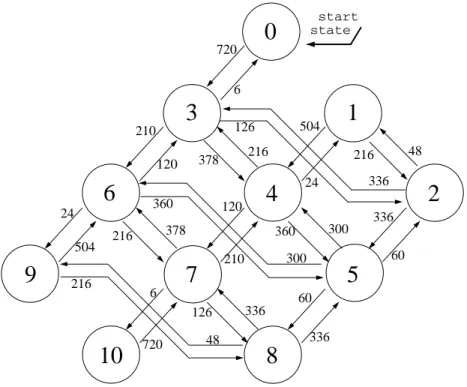
210 24 120 216 720 360 start state 126 378 504 48 216 336 60 336 336 60 300 360 300 336 126 48 216 720 6 210 120 24 6 504 216 378Figure 2: The Markov chain M for N = 10 states. The start state is state 0. Divide the number labeling each arc i→j byN =N(N −1)(N−2) = 720to get the transition probabilityPij.
the three will have to land in one of theibuckets that has an odd number of balls already, while the remaining two balls must land among theN−iremaining buckets. There are 3i(N−i)(N−i−1) ordered triples of bucket indices that will accomplish this among the N ordered triples of bucket indices. (The “3” takes care of the fact that there are 3i ways to choose the ball which lands in a bucket with an odd number of balls; after that ball is selected, the remaining two balls have to land in the otherN −ibuckets.) The reasoning for all of the other Pij values is similar.
In Figure 2 we depict the Markov chain M for some the case where the number of states is
N = 10. The transition probabilities are computed from Equation 1.
Using M to bound δ4. We are now ready to show that δ4 ≤ B(N). Recall that B(N) = λ(N)·β(N), where λ(N) and β(N) are given by the formulas in the statement of Theorem 7. Lemma 10 δ4 ≤ B(N).
Proof: First some notation. Let t ≤n be a number and let h1· · ·ht be a sequence of triples of distinct elements drawn from{1, . . . , N}. We make the following definitions.
• Parity(h1· · ·ht) is theN-vector whosei-th component,i∈ {1, . . . , N}, is 0 ifioccurs an even number of times in the multiseth1∪ · · · ∪ht, and 1 ifioccurs an odd number of times. (Thus
Parity(h1· · ·ht) records the parity of the number of balls in each of the N buckets, if we toss balls according toh1, . . . , ht.)
• Given anN-vector of bitsy=y1· · ·yN, let NumOnes(y) denote the number of 1-bits in y.
• Define State(h1· · ·ht) =NumOnes(Parity(h1· · ·ht)). (Thus State(h1. . . ht) records the state of M after hashing 1t with h = h1· · ·ht· · ·. After tossing balls according to h1, . . . , ht,
State(h1. . . ht) buckets contain an odd number of balls while N −State(h1. . . ht) buckets contain an even number of balls.)
• For σ an N-vector of bits, define Stateσ(h1· · ·ht) = NumOnes(σ⊕Parity(h1· · ·ht)). (Thus
Stateσ(h1. . . ht) captures the state ofM after hashing1t withh=h1· · ·ht· · ·, given that we start in the configuration specified byσ.)
• Let Hist(h1h2· · ·ht) = 0 State(h1) State(h1h2) · · · State(h1h2· · ·ht−1) State(h1h2· · ·ht) .
This is a list oft+ 1 numbers, each in{0,· · ·, N}, and it encodes the sequence of states inM
one passes through on hashing1t according to h=h1h2· · ·ht· · ·.
• LetDistinct(h1· · ·ht) betrue ifh1, . . . , ht are all distinct, andfalse otherwise.
• Let Rt (“random”) be the uniform distribution on h1,· · ·, ht (that is, each hi is a random triple of distinct points from{1, . . . , N}).
• Let Dt (“distinct”) be the uniform distribution on distinct h1, . . . , ht (that is, each hi is a random triple of distinct points from{1, . . . , N}, and no two of these triples are identical).
• Let C(m, t) denote the probability of at least one collision in the experiment of throwing t
balls, independently and at random, intom bins. We are now ready to prove the lemma.
δ4 = Pr D4[State(h1h2h3h4) = 0] = Pr R4[State(h1h2h3h4) = 0|Distinct(h1h2h3h4)] = Pr
R4[State(h1h2h3h4) = 0 andDistinct(h1h2h3h4)] Pr R4[Distinct(h1h2h3h4)] ≤ Pr R4[Hist(h1h2h3h4) {03630, 03430, 03230}] 1−C(N3, 4) (2) ≤ λ(N)· Pr R4[Hist(h1h2h3h4) = 03630] + PrR4[Hist(h1h2h3h4) = 03430] + Pr R4[Hist(h1h2h3h4) = 03230] = λ(N)· P03P36P63P30 + P03P34P43P30 + P03P32P23P30 = λ(N)·1·(N−3)(N−4)(N−5) N · 120 N · 6 N + 1· 9(N−3)(N−4) N · 36(N−4) N · 6 N + 1·18(N−3) N · 6(N−2)(N−3) N · 6 N (3) = λ(N)·720(N−3)(N−4)(N−5)+1944(N−3)(N−4) 2+648(N−2)(N−3)2 N3
= B(N)
Equation 2 is justified by referring to Figure 2: the only length-4 routes from state 0 back to state 0 are 03630, 03430, 03230, and 03030. The last of these can only arise from non-distincth1, h2, h3, h4. For the other three we simply disregard the conjunction with Distinct(h1h2h3h4) because we are giving an upper bound. Equation 3 is obtained directly from Equation 1. ♦
Using M to bound δ6, δ8,· · ·. Assume that N is even and N ≥6. We will show, in this case,
that δt ≤ B(N). Here is the idea. Take a random function h ∈ B and look at it’s last 6 maps— for convenience of notation, we write h = h7· · ·ht h1h2h3h4h5h6, numbering the final 6 maps h1, . . . , h6. Now h1, . . . , h6 are statistically correlated to h7, . . . , ht (for example, h1 = h7), yet
h1, . . . , h6 are nottoo far from being random and independent, in the sense that, for any h7· · ·ht, a uniformly selected sequence of maps h1h2h3h4h5h6 would have been a valid continuation with probability at least 1/2. (This follows from our assumption thatn≤N3/12.) Thus, up to a factor of 2, we can bound the chance of landing in state 0 on applyinghto1t by looking at the chance of landing in state 0 after applying a uniformly selectedh1. . . h6starting in some arbitrary (unknown) state of the Markov chain.
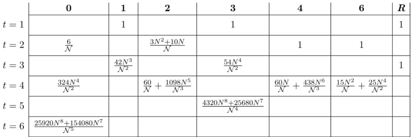
To formalize the above argument, let fi(t) denote the maximum, over all initial statess, of the probability that we arrive in stateiin exactly ttransitions, given that we start in state s. This is the same as the supremum, over all distributions π on the starting state of M, of the probability that we arrive in stateiin exactlyttransitions, given that we start in an initial state as chosen by sampling from π. We will need the following lemma about the behavior of Markov chainM. Lemma 11 f0(6)≤(25920N8+ 154080N7)/N5.
The proof is a tedious but straightforward calculation using the transition probabilities ofM. It is relegated to Appendix A. The point isn’t the specific formula, but only thatf0(6) is less than half
B(N) for all sufficiently largeN.
Lemma 12 Assume 6≤t≤n. Then δt≤B(N).
Proof: We use the same notation as in the proof of Lemma 10.
δt = Pr h∈B[h(1t) =0)] = Pr h7···hth1h2h3h4h5h6∈Dt[State(h7· · ·ht h1h2h3h4h5h6) = 0] = E h7···ht∈Dt−6 ⎡ ⎢ ⎣ Pr h1···h6∈D6 {h1,···,h6}∩{h7,···,ht}=∅ [State(h7· · ·ht h1h2h3h4h5h6) = 0] ⎤ ⎥ ⎦ ≤ max h7···ht∈Dt−6 h1···Prh6∈D6 {h1,···,h6}∩{h7,···,ht}=∅
[NumOnes(Parity(h7· · ·ht)⊕Parity(h1h2h3h4h5h6)) = 0]
= Pr
where E and σ are defined by fixing some h7· · ·ht which maximize the probability above and then letting σ =Parity(h7· · ·ht) and letting E be the uniform distribution on h1· · ·h6 subject to h1, . . . , h6 being distinct from all ofh7, . . . , ht and distinct from each other. Continuing, the above expression is:
=
Pr
h1···h6∈R6[Stateσ(h1h2h3h4h5h6) = 0 and Distinct(h1· · ·h6 h7· · ·ht)] Pr h1···h6∈D6[Distinct(h1h2h3h4h5h6 h7· · ·ht)] ≤ Pr h1···h6∈R6[Stateσ(h1h2h3h4h5h6) = 0] 1−6 t/N3 ≤ 2· Pr
h1···h6∈R6[Stateσ(h1h2h3h4h5h6) = 0] //From assumption thatn≤ N 3 /12 ≤ 2·f0(6) //Definition off ≤ 2·(25920N8+ 154080N7)/N5 //By Lemma 11 ≤ B(N) for allN ≥32
For the last inequality: it is easy to verify that this holds for sufficiently large N. The crossover
point was determined numerically. ♦
We have now shown that, under the conditions of the theorem, B(N) ≥ δt for all t ≥ 1. This completes the proof.
5
From Universal Hash Families to Message Authentication
In this section we review the Wegman-Carter construction (and its complexity-theoretic variant), as well as the formal notion of a message authentication code (MAC) and a pseudorandom function family.
MACs. We follow [14, 5] and define deterministic, counter-based message authentication codes.
A MAC scheme M specifies: constants L and c, determining Messages = {0,1}≤L and Tags =
{0,1}c; a set of strings Keys; a number MAX (alternatively, MAX = ∞); and a pair of functions (MAC,MACV), where
MAC : Keys×Messages× {1, . . . ,MAX} →Tags, and MACV : Keys×Messages×Tags→ {0,1}.
The first argument to MAC and MACV will usually be written as a subscript. We demand that for anyx∈Messages,k∈Keys, and cnt∈ {1, . . . ,MAX}, MACVk(x,MACk(x,cnt)) = 1 .
LetMbe a message authentication scheme. A MAC oracle MACk(·) forMbehaves as follows: it answers its first query,x1, with MACk(x1,1); it answers its second query,x2, with MACk(x2,2);
and so forth. The MAC oracle responds with the empty string to queries beyond theMAXth or to queries not in the setMessages.
An adversaryE for a message authentication schemeMis an algorithm equipped with a MAC oracle MACk(·). AdversaryEis said to forge on a particular execution, this execution having MAC
oracle MACk(·), if E outputs a string (x∗, σ∗) where MACVk(x∗, σ∗) = 1 yet E made no oracle query of x∗. When we speak of E forging with a particular probability, that probability is taken overE’s coin tosses and a random keyk∈Keys for the MAC oracle. Running times are measured in a standard RAM model of computation, with oracle queries counting as one step. By convention, the running time ofE also includes the size ofE’s description.
One can also provide the adversary with a MACVk(·,·) oracle, but this leaves the notion essen-tially unchanged.
The Wegman-Carter Construction. Given a family of hash functionsH={A→ {0,1}b}we
wish to construct from it a MAC. In the scheme we denote WC[H], the Signer and Verifier share a random elementh∈ H, as well as an infinite random stringP =P1P2P3· · ·, where|Pi|=b. The pair (h, P) is the key shared by the Signer and Verifier. The signer maintains a counter, cnt, which is initially 0. To generate a MAC for the messagex the signer increments cnt and then computes the MACσ = (cnt, Pcnt⊕h(x)) which authenticatesx. To verify a MACσ = (i, s) for the messagex
the Verifier checks ifs=Pi⊕h(x).
The following theorem says that it is impossible (regardless of time, number of queries, or amount of MACed text) to forge with probability exceeding the collision probability.
Proposition 13 [32, 18] LetHbe-AXU2 and suppose adversaryE forges in the schemeWC[H]
with probabilityδ. Then δ ≤.
PRFs. We follow [13, 5]. A finite pseudorandom function family (PRF) is a map F : {0,1}κ× {0,1}l → {0,1}b. We write Fa(x) in place ofF(a, x). LetRl,b be the set of all functions mapping
{0,1}l to{0,1}b. Adistinguisher is an algorithmD with access to an oracle. We say that a PRF
F is (t, q)-secure if for every distinguisher D which runs in time t and makes q or fewer queries to its oracle, Pr k←{0,1}κ DFk(·)= 1− Pr ρ←Rl,b Dρ(·)= 1
≤ (t, q) . Running times are measured in a standard RAM model of computation, with oracle queries counting as one step. By convention, the running time ofE also includes the size ofE’s description.
Wegman-Carter with a PRF. A natural complexity-theoretic variant is to use, instead of the
random pad P, a random index a∈ {0,1}κ into a finite PRFF :{0,1}κ× {0,1}l→ {0,1}b. The Signer maintains a counter cnt ∈ {0,1}l, initially 0. (We will not distinguish between numbers and their binary encodings into l-bits.) The Signer and Verifier share a random a ∈ {0,1}κ and a random h ∈ H. When the Signer wishes to MAC a message x, if cnt <2l−1 then the Signer computes σ = (cnt, Fa(cnt)⊕h(x)) and increments cnt. (In the unlikely event that cnt reaches 2l−1, a new MAC key is required by the Signer and Verifier.) To verify a MAC σ= (i, s) for the message x the Verifier checks ifs=Fa(i)⊕h(x). At most 2l messages may be MACed (after that, the key amust be changed). We call the scheme just described WC[H, F]. The following result is obtained by standard techniques.
Proposition 14 LetH={h:A→ {0,1}b}be an-AXU2 family of hash functions. LetTH denote the time required to compute a representation of a random element h∈ H, and let Th(q, μ) denote
the time required to compute from this representation the hash of q strings, these strings totaling
μ bits. Let F :{0,1}κ× {0,1}l → {0,1}b be an (t, q)-secure finite PRF. Let E be an adversary which, in time t, making q queries, these queries totaling μ bits, forges with probability δ against the scheme WC[H, F]. Then δ≤+(t+ Δt, q+ 1), where Δt=O(Th(q, μ) +TH+ql+qb).
The value of Δt would usually be insignificant compared to t. Note that in Proposition 13 the forging probability is independent of the number of queries (q) and the length of the queried messages (μ). In Proposition 14 the forging probability depends on these quantities only insofar as they are detrimental to the security of the underlying PRF.
We emphasize that the Signer is stateful in the schemes WC[H] and WC[H, F]. The Signer being stateful improves security (compared with using a random index) and at little practical cost. Note that the Verifier is not stateful. This is possible because our notion of MAC security (Section 5), does not credit the adversary for “replay attacks.”
6
Toy Example, and Limitations on Bucket Hashing
In this section we describe a concrete MAC based on the ideas presented so far. This is only a “toy” example; doing a good job at specifying a software-optimized bucket hash MAC would involve much design, experimental, and theoretical work which we have not carried out. Still, the example helps to illustrate the strengths of bucket hashing in making a MAC, as well as the limitations.
Toy Example. To keep things simple, suppose the strings we will MAC are of length at most
most 4096 bytes. Assume a word size of 4 bytes (32 bits). Let F :{0,1}κ× {0,1}64→ {0,1}64 be a finite PRF (defined, for example, from the compression function of MD5). Here is a way for the Signer to MAC a stringX whose length is at most 1024 words. Assume an even number of words. The Signer and Verifier share as a MAC key (i) a random element h1 ∈ B[32,1024,140], (ii) a random element h2 ∈ K[71,64], and a (iii) a random string a ∈ {0,1}κ. We use the construction of Proposition 5 (slightly modified to account for length-variability). In the algorithm below, |X|
denotes the length of X, encoded as a 2-word string. The function h1 is extended to strings of length less than 1024 words in the natural way: we stop casting words into buckets when we reach the end of the string. (This is equivalent to 0-padding the string to 1024 words.)
AlgorithmTOY-MAC(X).
if cnt = 264−1 then return error σ = cnt, Fa(cnt)⊕h2(|X|. h1(X))
cnt = cnt + 1 return σ
Let us count instructions for TOY-MAC to hash a 4096-byte message. If we bucket hash in 10 instructions per word (Section 3.3), hash using h2 ∈ K in 24 instruction per word ([24]), and compute F with 600 instructions (easy to accomplish), then we will spend 10 + (142/1024)·24 + 600/1024 = 10 + 3.3 + 0.6 = 13.9 instructions/word.
Notice that the “cryptographic” contribution to the above time (i.e., the time to compute F) is very small. In a Wegman-Carter MAC one is afforded the luxury of conservative (and slow) cryptography even in an aggressively speed-optimized design. This is because one arranges that the time to compute the MAC is dominated by the non-cryptographic work.
Limitations on bucket hashing. If the strings we are MACing are short then, at some point,
it makes sense to switch strategies and stop using bucket hashing. In our TOY-MAC, we might hash with onlyh2 when the input string has length less than some constant. This is an important limitation on bucket hashing; because the output length is substantial, the technique is simply not useful until the strings to be hashed get long enough. As a consequence, any “real” MAC which
employs bucket hashing would likely be a patchwork of different techniques for different message lengths. Therefore a real bucket hash MAC is unlikely to be simple to describe or implement.
On the other hand, if the strings to be hashed arevery long then, at some point, it makes sense to break the input into blocks and independently bucket has each block, using the construction of Proposition 2. This is because the size of the description of h ∈ B grows linearly in the maximal length string whichh can hash. We do not want hash functions with excessively long descriptions (certainly the hash function should fit in cache). This is another limitation on the bucket hashing technique, and something which will further complicate the definition of any real bucket hash MAC. In our TOY-MAC, if we wanted a substantially better collision probability we could apply the construction of Proposition 3, but this would roughly halve the rate for bucket hashing, and perhaps other techniques might then be faster. This is a third limitation on bucket hashing: until better constructions are found, obtaining an extremely small collision probability, say 2−50, would require an excessive number of buckets. That is, the output length of the hash function would be very long, and so the technique would only be useful for hashing extremely long messages.
The last limitation we will mention is the time needed to compute a description ofh. In any real MAC scheme the functionh∈ Bwould be determined from some underlying keykwith the help of a pseudorandom generator. Because the description ofhis large and of a special form, computingh
might take a significant amount of time. In most applications of fast message authentications, a one-time key pre-processing delay is not important. But if there is a limited amount of text to be MACed, or if the latency of the first MAC must be minimized, than the time to compute the description of h could be an issue. One approach is to find a version of bucket hashing that uses a small key (ie., a short description for h). This way the underlying pseudorandom generator (if present) is less taxed. This approach has been investigated by [16], who achieves a major reduction in the size of the description theh.
Balanced against these limitations is the possibility of extremely high MAC throughput, at least for long strings.
7
Extensions and Directions
GeneralizingB, we call by “bucket hashing” any scheme in which the hash functionhis a given by a list h1· · ·hn of “small” subsets of{1, . . . , N}and the hash ofX =X1· · ·Xn, where|Xi|=w, is:
for j←1 to N do Yj ←0w for i←1 to n do
for each k∈hi do
Yk ←Yk⊕Xi
return Y1Y2 · · · YN
In the general case the distribution on h-values is arbitrary. So B is just the special case in which we use the uniform distribution on distinct triples in{1, . . . , N}.
One could imagine many alternative distributions, some of which will give rise to faster-to-compute hash functions or better bounds on the collision probability. As an example, suppose
h∈ H is chosen by randomly re-ordering a list h1· · ·hn of triples which are chosen so that for all sets I ⊆ {1, . . . , n} of cardinality 2 or 4, it is not the case that the multiset ∪h∈Ih has an even number of each point 1, . . . , N. This new family of hash functions may have substantially smaller collision probability than Bfor a given n, N.
The bucket hash scheme of a graph. Hash family Bwould have been more efficient had each
word gone into two buckets instead of three. One way to specify a scheme where each word lands in two buckets is with a graph G whose N vertices comprise the N buckets and whose m edges
{1, . . . , m} indicate the pairs of buckets into which a word may fall. A random hash function from the family is given by a random permutation π on {1, . . . , m}. To hash a string X1. . . Xn using
π, where |Xi|=w and n≤m, each word Xi is dropped into the two buckets at the endpoints of edge π(i). As before, we xor the contents of each bucket and output their concatenation in some canonical order. We call the above scheme the bucket hash of the graph G.
For a graph Gto be “good” we want a small number of verticesN, a large number of edgesm, and such that for all k where 1≤k ≤n≤m, if k distinct edges are selected at random from G, then the probability that their union (with multiplicities) comprises a union of cycles is at most some tiny number.
One possible choice of graphs in this regard are the (d, g)-cages (see [8]). A (d, g)-cage is a smallest d-regular graph whose shortest cycle has g edges. These graphs have been explicitly constructed for various values of (d, g). Though (d, g)-cages are rather large (for even g they have at least (2(d−1)g/2−2)/(d−2) nodes) and the definition of a (d, g)-cage does not exactly correspond to having small collision probability, we conjecture that some (d, g)-cages may still give rise to useful hash families. For example, assume d−1 is a prime power. Let C[d,6] be the (d,6)-cage. This is the the point-line incidence graph of the projective plane of order d−1. Bucket hashing with
C[10,6] may be a good way to hash 909 words down to 182 words.
Open questions. The generalized notion of bucket hashing amounts to saying that hashing
is achieved for each bit position 1. . . w by matrix multiplication with a sparse Boolean ma-trix H. Expressing the method in this generality raises questions like the following: for a given
N, n and k, for what distributions D of binary N ×n matrices H having k ones per column is maxx∈{0,1}n−{0n} Pr
H∈D[Hx=0] minimized? What if we also demand that each row has a fixed number of ones? What if, instead of saying that there are kones per column, we cap the density of the matrix at some valueρ? Answers to such questions may lead to faster bucket hash schemes. Acknowledgments
Many thanks to the two anonymous referees for their careful reviews. Thanks also to Mihir Bellare, Don Coppersmith, Hugo Krawczyk, and David Zuckerman for their comments and suggestions.
This work was supported in part by NSF CCR-9624560.
References
[1] N. Alon, O. Goldreich, J. H˚astad and R. Peralta, Simple constructions of almost k-wise independent random variables, 31st Annual Symposium on Foundations of Computer Science, IEEE Computer Society, 1990, pp. 544–553.
[2] R. Arnold and D. Coppersmith, An alternative to perfect hashing, IBM RC 10332 (1984). [3] M. Bellare, R. Canetti and H. Krawczyk, Keying hash functions for message
authentica-tion,Advances in Cryptology – CRYPTO ’96, Lecture Notes in Computer Science, vol. 1109, Springer-Verlag, 1996, pp. 1–15.
![Figure 1: A graphical representation of Theorem 7. We plot of N verses, B(N ), our bound on the collision probability of B[w, n, N].](https://thumb-us.123doks.com/thumbv2/123dok_us/9867677.2876513/8.918.190.714.119.497/figure-graphical-representation-theorem-verses-bound-collision-probability.webp)