DESIGN OF MODEL PREDICTIVE CONTROLLER BASED MULTI OBJECTIVE PSO AND TS MODELLING APPROACH

1500

AUTOMATED SHORELINE DETECTION DERIVED FROM

VIDEO IMAGERY USING MULTI THRESHOLDING

TECHNIQUES

1_{I M.O. WIDYANTARA,} 2_{I N. ARMAWAN,} 3_{I M.D.P. ASANA,} 4_{I B.P. ADNYANA} 1,2_{Electrical Engineering Department, Engineering Faculty, Udayana University, Indonesia}

3_{Informatic Department, STMIK STIKOM Indonesia, Indonesia} 4_{Department of Civil Engineering, Udayana University, Indonesia}

E-mail: 1_{[email protected],} 2_{[email protected],} 3_{[email protected],} 4_{[email protected]}

ABSTRACT

Shoreline is a zone of contact between the ocean and the land which always changes due to the movement of sediment across the coast. Dynamic changes in shoreline can cause abrasion and accretion which can damage the coastal environment. Therefore, monitoring the position of the shoreline is a very significant issue given the socio-economic value and high population density along shore areas. This paper presents a new approach in automated shorelines detection based on video images. Several sequences of image processing with the main component being image segmentation using Harmony Search Multithresholding Algorithm (HSMA) are employed. This algorithm combines the original harmony search algorithm (HSA) and the Kapur’s algorithm as an objective function to obtain the optimum threshold value in order to improve the quality of segmentation. A series of advanced image processing steps are also applied to the segmented images, mainly binarization, morphological operation, and Canny edge detection for land/sea object classification. The final product of the image processing chain is the continuous line coverage that is visualized as a shoreline. Based on the results of testing carried out on several video images, the proposed method is able to accurately detect shorelines along the borders of land and sea objects.

Keywords: Video Monitoring, Shoreline Detection, Harmony Search Algorithm, Canny Edge Detection, Morphological Operation, Coastal Management.

1. INTRODUCTION

At present, our coastal territory has experienced a potentially decline in environmental quality due to natural events and environmental exploitation by humans, such as sedimentation, erosion, sea level rise and tidal flooding. This ongoing erosion have negative impacts on civilizations that surrounding coastal areas. Therefore, coastal zone monitoring is very important to be carried out as an effort to manage coastal resource management and coastal environmental protection[1][2].

Remote sensing video system is a monitoring technique that utilizes video camera devices as visual sensors. Video based monitoring offers flexibility in installation, low cost, and ability to produce continuous monitoring images with greater temporal and spatial sampling frequencies. Therefore, a video monitoring system based on digital image processing techniques is an optimal instrument to get an

objective shoreline position [3]. Accurate identification of shoreline positions is important information for coastal scientists, managers and engineers in coastal zone management of expected climate change [4][5].

In video-based coastal monitoring systems, shoreline detection is a complex work related to physical conditions during image capture, such as the position of camera placement, camera sensor capabilities and weather phenomena. When a video camera is installed in a place that is not too high, the characteristics of the resulting image will always change due to wind conditions, local currents and changes in the depth of the sea. Therefore, the main problem in the coastline detection process is obtaining a reliable image processing technique to obtain clustering of land and sea areas.

1501 monitoring approach [6]. In coastal imagery, the evolution of significant dynamic beach features can be identified/recorded, such as the wet/dry beach interface, the last breakwater line (the deepest coast), or the swash zone boundary. All of these features can be used as proxies for horizontal shoreline positions, and inspired many researchers to develop various image processing algorithms for shoreline extraction.

A review of the shoreline extraction algorithm has been carried out by Plant et al. [7]. This study has

demonstrated the challenges associated with developing universal and strong automatic shoreline extraction procedures from coastal images, mainly due to the high temporal (intra-annual) variability of the coastal, hydrodynamic, and morphological conditions. This research framework has been intensively modified by researchers to obtain shoreline extraction and data quality control to overcome high regional and temporal beach variability [8][9][10].

The shoreline extraction with binary classification on coastal images using a meaningful neural network approach has been proposed by Kingston [11] and Vousdoukas et al. [10]. In [11], shoreline

identification is based on discrimination of wet area pixels from dry area pixels on binary images using a standard feed-forward neural network (FFNN), which is trained with backpropagation gradient-descent algorithms. While in [10], land area classification is obtained from feature extraction of image histograms which are parameterized by non-linear image histogram function.

A very similar approach was proposed by Rigos et al. [12][13], by distinguishing the functions used for

histograms and ANNs. In [10], after the thresholding-based segmentation process, the histogram of the variant image is approximated by the Chebyshev polynomial function. To improve the accuracy of the histogram, Rigos et al. [12][13]

implement the Radial Basis Function (RBF) network so that the number of polynomial coefficients can define the dimensions of the input space. Clustering analysis based on Fuzzy c-means has been used to determine the center of RBF, and the weights of hidden nodes are calculated using the steepest descent approach.

In the framework of the beach video monitoring system, Valentini et al. [14][15] has proposed a tool

that automatically forms shoreline detection and data analysis. The proposed Shoreline Detection Model (SDM) is compiled by shoreline detection routines that are implemented in web applications, including

image processing (i.e. shoreline extraction and geo-rectification), data analysis, and dissemination of coastal evolution in quasi-real time.

The approaches proposed above rely on the shoreline detection performance in the thresholding segmentation method based on the image histogram. In the thresholding approach, the coastal image is partitioned into several classes based on the predetermined threshold value. Therefore, each class has a different segmentation quality. To improve the quality of segmentation, an optimization method called harmony search multithresholding algorithm (HSMA) has been proposed by Oliva et al.[16]. This

algorithm combines the original Harmony Search Algorithm (HSA) with the Otsu [17] and Kapur methodology [18]. Compared to other optimization algorithms such as Genetic algorithm (GA)[19], Particle Swam Optimization (PSO) [20], and Bacterial Foraging algorithm (BFA)[21], HSMA is able to improve the quality of image segmentation.

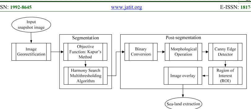
This paper describes an automatic shoreline detection approach from video images. This approach consists of several sequences of image processing, with the main component being image segmentation using Harmony Search Multithresholding Algorithm (HSMA). The goal is to improve the quality of segmentation images by optimizing the threshold value. Shoreline detection is done by extracting objects in the segmentation image using several processes including binarization, morphological operation, and Canny edge detection [22] for classification of land / sea objects. By exploiting the best elements of the algorithm from previous studies, the proposed approach is comprehensively capable of automatically detecting shorelines

2. METHODOLOGY OVERVIEW

1502

Figure 1: The Proposed Shoreline Detection System Framework

in the image before applying the shoreline extraction method.

3. IMAGE SEGMENTATION USING

HARMONY SEARCH MULTI

TRESHOLDING

First step in detecting the shoreline is the segmentation of objects in the coastal image. In coastal video image segmentation, images are partitioned into different classes and each of these classes has different segmentation qualities. To overcome variations in image quality and image opaque areas, multilevel thresholding techniques with optimization algorithms can be used to select the optimum threshold values. Choosing an optimum threshold until the threshold does not experience change is important in segmentation. Multithresholding (MT) segmentation techniques optimize the threshold values using an optimization algorithm with objective functions. The aim is to improve the quality and accuracy of segmentation images using a multilevel threshold technique.

Some thresholding techniques have been proposed by several researchers, such as Otsu [17] who maximize variance between classes, and Kapur et al

[18] which maximizes entropy to measure homogeneity between classes. The efficiency and accuracy of these techniques have been proven for bilevel segmentation [23]. Although this technique can be extended to MT, the complexity of the computation will increase exponentially when a new threshold is entered [24]. Furthermore, Olive et al

[16] have proposed an MT technique based on harmony search algorithm (HSA), hereinafter referred to as harmony search multithresholding algorithm (HSMA). This algorithm combines the original harmony search algorithm (HSA) with the Otsu and Kapur methodology. This proposed

algorithm takes a random sample from a decent search space in the image histogram. The samples build each harmony (candidate solution) in the context of HSA, while the quality is evaluated using the Otsu’s or Kapur’s objective function. Guided by these objective values, a series of candidate solutions are developed using HSA operators until an optimal solution is found. This approach produces a multilevel segmentation algorithm that can effectively identify the threshold value of digital images with a reduced number of iterations. Based on the efficiency of HSMA, this paper uses it as a coastal image segmentation method that has been georectified.

3.1 Kapur’s Objective Function Method

Kapur et al. [18] has proposed a nonparametric

method for determining the optimal threshold (th)

value, based on the entropy and probability distribution of the image histogram. In principle, the Kapur method looks for the optimal th value to

maximize the overall entropy. Entropy in an image represents a measure of compactness and separation between classes. Therefore, when the optimal th

value precisely separates the class, then entropy has the maximum value.

Assume that I is a digital coastal video image

which is stated in Red, Green and Blue (RGB) components or Gray scale, and each has an intensity value (i) in the range [0, L-1]. The histogram of each

component is made by counting pixels with the same component intensity. The histogram is expressed as

hc_{(i), with c is the component of the image which}

depends if the image is gray scale or RGB, dan i =

0,1, …, L-1. The probability of the pixels in

component c at level i is Phci. If Nci is the number of pixels of component with level c with level i, the

probability of Phc

1503

1

, 1

1, 2,3 if RGB image 1 if Gray scale image

c NP

c i c

i i i h Ph Ph NP c       



where, NP is the dimension of the image. For bilevel segmentations, two classes are defined

 1    1  

1 2

0 0 1 1

,..., , ,...,

c c

c c

th th L

c c c c

Ph Ph

Ph Ph

C C

th th th th

   



  (2)

where 0(th) and 1(th) are probabilities

distributions for C1 and C2, each expressed as

 

 

0 1

1 1

,

th L

c c c c

i i

i i th

th Ph th Ph

 

  







Based on the concept of bilevel segmentation above, the objective function of the Kapur's problem can be defined as

 

1, 2,3 if RGB Image 1 if Gray scale image

c c

J th H H

c       (4)

where the entropies H1 dan H2 are computed by:

1

1 0 0

1

1 1 1

ln

ln

c c

th

c i i

c c

i

c c

th

c i i

c c i Ph Ph H Ph Ph H                    





Furthermore, for multiple threshold values, the objective function of the Kapur method can be expressed as

 

1

max ,

1,2,3 if RGB Image 1 if Gray scale image

k c i i

J TH H

c     _{ }      



where TH = [th1, th2, …., thk-1] is a vector that

contains the multiple thresholds. Each entropy is computed separately with its respective th value.

Therefore, the definition of entropy can be expanded to:

1

1

1

1

1 0 0

1

1 _{1 1}

1 1 1

ln , ln , . . ln i k c c th

c i i

c c

i

c c

th

c i i

c c

i th

c c

th

c i i

k c c

i th k k

Ph Ph H Ph Ph H Ph Ph H                 _{ }             _{ }  







where, the probability occurrence values (

0, 1,..., 1

c c c

k

  _ ) of the k classes are obtained using

1 2 1 0 1 1 1 1 1 ( ) ( ) . . ( ) k th c c i i th c c i i th L c c k i i th th Ph th Ph th Ph            







and the probabilitydistribution c i

Ph with (1). Finally,

the segmentation process to separate pixels into the appropriate class is done using the rules of

1 1

2 1 2

1

0 ,

,

,

1,

i i i

n n

C p if p th

C p if th p th

C p if th p th C p if th p L

              (9)

3.2 Harmony Search Multithresholding Algorithm

Harmony Search Algorithm (HSA) is used to optimize the threshold value. To segment coastal images, HSA is combined with Kapur’s objective function. HSA takes a random sample of possible search areas in the image histogram. These samples build each harmony (candidate solution), where the quality is evaluated using Kapur’s objective function. With this objective value, a set of candidate solutions are developed using HSA operators until an optimal solution is found. This approach produces a multilevel segmentation algorithm that can effectively identify the threshold values of coastal images in a reduced iteration range.

In the context of multithresholding, the combination of HSA and the objective function of Kapur’s is called HSMA, consists of three main phases, namely Harmony Memory (HM) initialization, improvisation of new harmony vectors, and updating HM.

A. Harmony Memory Initialilazation.

In this phase, the initial vector components in HM will be configured. Each Harmony (candidate solution) uses different elements as decision variables in the optimization algorithm. For segmentation, decision variables state a different threshold point (th). So, the HM matrix with

1504

1 2

1 1

, ,...., ,

, ,...., ,

c c c

HMS

c c c c

i k

HM x x x

x th th th

 

  

 

  

(10)

where T represents the transpose operator, HMS is

the size of HM, xi is the i element of HM, c = 1,2,3

for RGB images and c = 1 for gray scale images. Search space c

_{ }

i

x j is defined as a combination of

the upper and lower bounds, l(j) dan u(j), that is:

   



   



 

1, 2,..., 1, 2,...., c

i

x j l j u j l j rand

j n i HMS

  

 

(11)

In the multitresholding context, the search space limits set to l = 0 and u = 255 are associated with

image intensity levels.

B. Improvement of New Harmony Vectors.

In this phase, a new harmony vector (xnew) is

constructed by applying 3 (three) operators, namely: memory consideration, random reinitialization, and pitch adjustment. Using memory consideration operations and random reinitialization, the value of the xnew is expressed as:

 

 



   

 



 



   



 

1 , 2 ..., ,

with probability HMCR

. 0,1 ,

with probability 1- HMCR

i HMS

new

x j x j x j x j

x j

l j u j l j rand

                  (12)

where, the xnew(j) will be obtained through memory

consideration operation if the uniform random number is smaller than the Harmony Memory Consideration Rate (HMCR). Instead, it will be obtained through a random reinitialization between the search bound [l(j), u(j)].

Furthermore, the pitch-adjusting operation is used to control the local search around the selected elements of HM. The pitch-adjusting decision is calculated by:

 

 

 

 

 





0,1 . , with probability PAR , with probability 1 - PAR

new new

new

new

x j x j rand BW

x j x j         (13)

where PAR is the pitch-adjusting rate, and BW is the bandwidth factor.

C. Updating the Harmony Search.

At this stage, HM is updated by comparing the harmony of the new candidate xnew and worst

harmony vector (xw) in the HM. Vector xw is replaced

by xnew when the latter provides a better solution in

the HM. The process is repeated until there is no change in the value of fitness.

D. HSMA Implementations

Referring to [16], the HSMA segmentation algorithm is implemented with Kapur's objective function. The implementation of the algorithm is concluded as in Algorithm 1.

4. POST-SEGMENTATION PROCESSING 4.1 Binary Conversion

To identify the shoreline, the first step that must be done is to convert the image that has been segmented to binary image. The goal is to get the land and sea regions. The binary image b(i, j) is made

after the HSMA operation using the method proposed by [25]:

,

, 255, ( , ) ( , )

0 , ( , )

i j i j

if f i j th b i j

if f i j th  

  _

 (14)

where f(i, j) is the intensity value of the image pixel

on (i, j), and thi,j is the threshold value. Pixels with

an intensity value higher than the threshold encoded as 255 (land pixels), otherwise it is encoded as 0 (sea pixels)

4.2 Morphological Operation

Morphological operations are used to optimize the results of segmentation in binary image b(i, j) by

eliminating noise in objects that are not needed. Noise often appears in the form of small objects in regions of land or sea. Therefore, combining small objects into objects that have a greater intensity value can produce only two large objects, namely land and sea in binary images. Based on morphology operations, two stages of the process for improving binary image quality are:

A. Opening operation

Opening operation is a combination where a digital image is subjected to an erosion operation followed by a dilation. Dilation is the process of adding pixels to the boundary of an object in the input image, while erosion is the process of removing/reducing pixels at the boundary of an object. Opening operations in the image have the effect of smoothing object boundaries, separating objects that previously held together, and removing objects that are smaller than the size of structuring. Sequentially, dilation, erosion, and opening operations are stated as:

AB (15) A B (16)





1505

Algorithm 1

where A is the binary image b(i,j) and B is

structuring element.

B. Imfill Operation

For binary images, imfill operations convert connected background pixels (0s) to foreground pixels (1s), stopping when they reach object boundaries. The goal is to combine small objects into land objects.

4.3 Canny Edge Detector

Morphology operation in binary image b(i,j)

produces two large objects that are identified as land and sea regions. Furthermore, shoreline detection is done by extracting edge pixels at the borders of the two objects. Edge detection is the process of getting an area that has a sharp change in intensity in the image. This paper has proposed the Canny edge detection method with the Sobel operator as kernel convolution [22][26].

Canny edge detectors work in several processes. First, the image is smoothed with a Gaussian

convolution then the first two-dimensional derivative is checked by calculating the gradient magnitude (edge strength) and gradient direction. Convolution of the Gaussian Filter with the original image is stated by:

   

2 2

2

2

1

, * ,

2

i j

f i j e  b i j





 

 

_{ }

 

(18)

Next, the first-order derivative of an image f(i,j) in

location (i,j) is expressed as a two-dimensional

vector:

 , i

j

f

G _i

G f i j

f G

j



 

   

  _{ }

  _ 

  _{ }_

(19)

where,

   

   

, ,

, ,

f _{f i n j f i n j}

i

f _{f i j n f i j n}

j

 _{   }



 _{   }



(20) 1: For RGB images, save intensity levels to IR, IG, IB, while for gray scale images, save to

IGR. Define, c = 1, 2, 3 for RGB images or c = 1 for gray scale images.

2: Get a histogram from each image component: hR_{, h}G_{, h}B _{(RGB images), and h}GR _(gray

scale images).

3: Calculate the probability of Phc

i using (1) and obtain the histograms

4: Initialize a HM xc

i of HMS random particles with k dimensions.

5: Calculate the value c i and ci

6: Get a new harmony xc

new with the following procedures:

for (j = 1 to n) do

if (r1< HCMR) then xnewc  j xac j where a 1, 2,.., HMS if (r2 < PAR) then

    3.

c c

new a

x j x j r BW where r1, r2, r3 rand (0,1)

end if

if c    

new

x j l j

   

c new

x j l j

end if

if c    

new

x j u j

   

c new

x j u j

end if else

    .





c new

x j l j r u j l j where r  rand (0,1)

end if end for

7: Update harmony memory,

    .





c new

x j l j r u j l j , where r  rand (0,1)

8: If NI is satisfied, then jump to step 9, and vice versa return to step 5 9: Choose the harmony with the best xc

best value.

1506 where, n is a small integer and usually is unity. A

gradient magnitude and an edge orientation are expressed in equations (21) and (22), respectively.

 _, 2 2

i j

G f i j_  _ G G (21)

3 arctan

4

y x

G

G

   (22)

In its implementation, the Canny edge detector uses the Sobel operator as a gradient operator. The Sobel operator is a kernel convolution process that is used to restore a high response where there is a sharp change in the image gradient. This paper uses kernel pairs (33), each for Gi and Gj. The first kernel is

used to estimate the gradient in i-direction, and the

other is to estimate the gradient in j-direction. The

sobel Operator matrix used in this paper is shown inequation (25).

1 0 1 1 2 1 2 0 2 0 0 0 1 0 1 1 2 1

i j

G G

    

   

_{ }   

   

      

   

(23)

4.4 Region of Interest (ROI) and Image Overlay The Canny edge detection process to extract shorelines was carried out in the spatial image. This

process produces line detection on all edges of rectification images labeled as land. On the other hand, shoreline detection is intended to extract shorelines only along the border of land and water areas.

In an effort to extract the shoreline, this paper has applied the Region of Interest (ROI) technique as a marker positioned in the middle area of the image. ROI is done once for all images captured by the video camera in a fixed position. Furthermore, shoreline extraction in ROI is overlaid on rectification images to show shoreline visualization in rectification images.

5. RESULT AND DISCUSSION

The image used was obtained from an IP video camera mounted on the Cucukan beach in Gianyar regency, Bali Province, Indonesia. Video images have 1920  1080 pixels dan and are georectified using Pawlowicz Algorithm [27]. Georectification images are formed by applying between 8-10 GCPs and corresponding ICPs (Figure 2). These points are features that can be clearly identified in an image with its geographical position known. GCP position is expressed in GPS coordinates.

(a)

(b) (c)

1507 5.1 Segmentation Analysis

Aligned with Algorithm 1 adopts the HSMA parameter values that have been used in [16]. In the Harmony Memory Initialization phase, the values of the initial vector components in HSMA such as HM, HMCR, PAR, BW, and number of iterations (NI) are arranged as shown in Table 1. Furthermore, performance evaluation of the HSMA implementation is carried out in several simulation conditions including:

 The threshold levels (th) are set at 2.3, and 4.

 The Harmony update process will stop when the fitness value of the best harmony has reached 10% of NI.

 Evaluation of stability and consistency using standard deviation (STD), as shown in equation (24),

 

1

NI i i

bf av

STD

Ru

 





where, bfi is best fitness in the i iteration, av is

the average value of bf, and Ru is the total

number of executions.

 Quality evaluation uses a peak to peak signal to nose ratio (PSNR), as shown in the equation (25),

 

   





10

0 1 1

255 20log

, ,

ro co

c c

th i j

PSNR dB

RMSE

I i j I i j

RMSE

ro co  

 

 _{ }

 

 





(25)

where, 0

c

I is the original image,Ithcis segmented

image, co and ro are the number of rows and

columns of the image.

Tabel 1: HSMA Parameter Values

HM HMCR PAR BW NI

50 0.95 0.5 0.5 25,000

The performance of HSMA based on entropy function as objective function is shown in Tables 2 and 3. The values evaluated are PSNR, STD, and the best threshold value in the last population ( B

t

x ).

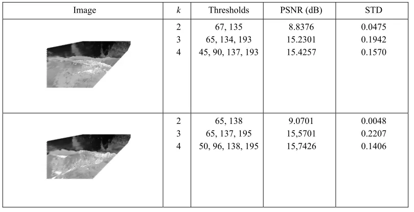
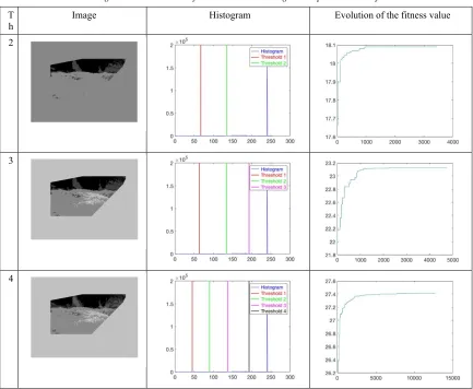
Visually, the segmented image at each threshold value is associated with its histogram value and the evolution of its fitness value during the execution of the HSMA method. All results have shown that the addition of the threshold value can increase the PSNR and STD values. Therefore, to produce a good regional classification, this study uses a threshold value (th) equal to 4 for the entire segmentation process of the shoreline detection system.

5.2 Shoreline Detection Analysis

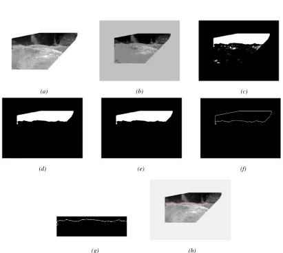
Figure 6 shows the automatic extraction of shorelines from video images that have been georectified. Binarization of segmentation image produces binary image outputs b(i,j) which have not

yet fully produced regions in the criteria of land and sea. There are small image objects in the sea area indicated as land area (Figure 6c). Therefore, a mechanism is needed to combine these small picture objects and label them to the land or sea area.

Morphological techniques with opening operations are carried out to eliminate small objects

Table 2: Evaluation of Segmentation Quality After Applying The HSMA

Image k Thresholds PSNR (dB) STD

2 3 4

67, 135 65, 134, 193 45, 90, 137, 193

8.8376 15.2301 15.4257

0.0475 0.1942 0.1570

2 3 4

65, 138 65, 137, 195 50, 96, 138, 195

9.0701 15,5701 15,7426

1508

Table 3: Histogram And Evolution Of Fitness Values During The Implementation of The HSMA

T

h Image Histogram Evolution of the fitness value

2

3

4

that are in the ocean region in binary imagery b(i, j).

By combining erosion and dilation operations, the opening operation has merged and eliminated small objects in the ocean region (Figure 6(d)). In this case, the structure element used is a box type of 8  8 pixels. In the same case in the land region, the implementation of imfill operations is able to convert backgoround pixels (0's) to foreground pixels (1's). The application of both operations has resulted in binary images with two large objects, namely land and sea (Figure 6(e)).

The shoreline detection in Figure 6(e) is done by extracting the edges of the image along the land and sea objects using the Canny edge detection algorithm. The two main parameters that must be considered in the implementation of the Canny algorithm are the standard deviation of the Gaussian function, and the low and high threshold values for classifying edge pixels as strong or weak. This study has used a standard deviation equal to 1, and the threshold values for low and high are 0.4 and 0.7 respectively. Canny edge extraction has produced a

continuous line along the land object (Figure 6 (f)). This result is understandable because that objects in the geo-rectification image are in a picture frame with a resolution of 19201080 pixels, so the Canny algorithm performs the extraction process in all pixels.

Furthermore, the shoreline detection process is carried out by determining the ROI position in the area with the coastline only between the land and sea objects. In this paper, the ROI position is fixed for all coastal images processed by the shoreline detection system. Therefore, the detection of the final coastline is obtained in the area in ROI (Figure 6 (g)). The final process to produce the shoreline image is by overlaying the ROI image to a georectified image, as shown in Figure 6 (h).

pre-1509

(a) (b) (c)

(d) (e) (f)

(g) (h)

Figure 6: The shorelines extraction and detection processes, (a) Rectified image, (b) Segmented image, (c) Binarization, (d) remove small object, (d) fill hole in region, (f) Canny edge detection, (g) ROI, (h) Shoreline image

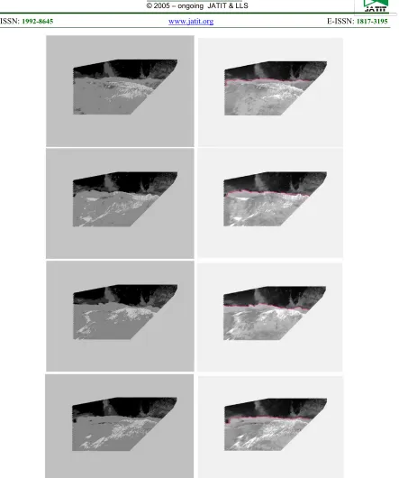
segmentation, segmentation and post-segmentation process are fixed to produce a shoreline detection system automatically. As shown in Figure 7, the proposed shoreline detection system is able to detect shorelines continuously. This has shown that the HSMA segmentation algorithm is able to cluster land and sea areas well on various characteristics of coastal imagery. Furthermore, the post-segmentation method based on Canny edge detection is also capable of carrying out shoreline extraction and detection processes properly.

6. CONCLUSION

A new automatic algorithm for extraction and detection of shorelines in video images has been presented. The algorithm is developed in two main modules, namely segmentation and post-segmentation. The segmentation of georectification images was carried out with HSMA based Kapur's function. Shoreline detection in post-segmentation is

done by extracting binary images through several process stages including binarization, morphological operations, Canny edge detection, ROI and imgae overlay. The results of experiments on several video images have shown that the proposed algorithm is able to detect and visualize the coastline continuously.

1510

Figure 7: Shoreline detection

ACKNOWLEDGMENT

This research was supported and financed by the ministry of technology research and higher education in the Republic of Indonesia with a contract number 171.86 /UN14.4.A/LT/2018.

REFRENCES:

[1] A.-M. Saeed and A.-M. Fatima, “Coastline Extraction using Satellite Imagery and Image Processing Techniques,” Int. J. Curr. Eng. Technol., vol. 6, no. 4, pp. 1245–1251, 2016. [2] C. A. Mello, T. J. Dos Santos, H. R. Medeiros, and

1511

[3] I. Turner et al., “Comparison of observed and predicted coastline changes at the gold coast artificial (surfing) reef, Sydney, Australia,” in Proceedings of the International Conference on Coastal Engineering, 2001.

[4] M. D. Harley and P. Ciavola, “Managing local coastal inundation risk using real-time forecasts and artificial dune placements,” Coast. Eng., vol. 77, pp. 77–90, 2013.

[5] M. Radermacher, M. Wengrove, J. S. M. Van Thiel de Vries, and R. Holman, “Applicability of video-derived bathymetry estimates to nearshore current model predictions,” Proc. 13th Int. Coast. Symp. Durb. South Afr. 13-17 April 2014 J. Coast. Res. Spec. Issue 70 2014, 2014.

[6] E. H. Boak and I. L. Turner, “Shoreline Definition and Detection: A Review,” J. Coast. Res., pp. 688–703, Jul. 2005.

[7] N. G. Plant and R. A. Holman, “Intertidal beach profile estimation using video images,” Mar. Geol., vol. 140, no. 1, pp. 1–24, Jul. 1997. [8] A. F. Osorio, R. Medina, and M. Gonzalez, “An

algorithm for the measurement of shoreline and intertidal beach profiles using video imagery: PSDM,” Comput. Geosci., vol. 46, pp. 196–207, 2012.

[9] M. I. Vousdoukas et al., “Performance of intertidal topography video monitoring of a meso-tidal reflective beach in South Portugal,” Ocean Dyn., vol. 61, no. 10, pp. 1521–1540, 2011.

[10] M. I. Vousdoukas, D. Wziatek, and L. P. Almeida, “Coastal vulnerability assessment based on video wave run-up observations at a mesotidal, steep-sloped beach,” Ocean Dyn., vol. 62, no. 1, pp. 123–137, 2012.

[11] K. S. Kingston, B. G. Ruessink, I. M. J. Van Enckevort, and M. A. Davidson, “Artificial neural network correction of remotely sensed sandbar location,” Mar. Geol., vol. 169, no. 1–2, pp. 137– 160, 2000.

[12] A. Rigos, G. E. Tsekouras, M. I. Vousdoukas, A. Chatzipavlis, and A. F. Velegrakis, “A Chebyshev polynomial radial basis function neural network for automated shoreline extraction from coastal imagery,” Integr. Comput.-Aided Eng., vol. 23, no. 2, pp. 141–160, 2016.

[13] A. Rigos, O. P. Andreadis, M. Andreas, M. I. Vousdoukas, G. E. Tsekouras, and A. Velegrakis, “Shoreline extraction from coastal images using Chebyshev polynomials and RBF neural networks,” in IFIP International Conference on

Artificial Intelligence Applications and

Innovations, 2014, pp. 593–603.

[14] N. Valentini, A. Saponieri, and L. Damiani, “A new video monitoring system in support of Coastal Zone Management at Apulia Region,

Italy,” Ocean Coast. Manag., vol. 142, pp. 122– 135, 2017

[15] N. Valentini, A. Saponieri, M. G. Molfetta, and L. Damiani, “New algorithms for shoreline monitoring from coastal video systems,” Earth Sci. Inform., vol. 10, no. 4, pp. 495–506, 2017. [16] D. Oliva, E. Cuevas, G. Pajares, D. Zaldivar, and

M. Perez-Cisneros, “Multilevel thresholding segmentation based on harmony search optimization,” J. Appl. Math., vol. 2013, 2013. [17] N. Otsu, “A threshold selection method from

gray-level histograms,” IEEE Trans. Syst. Man Cybern., vol. 9, no. 1, pp. 62–66, 1979.

[18] J. N. Kapur, P. K. Sahoo, and A. K. Wong, “A new method for gray-level picture thresholding using the entropy of the histogram,” Comput. Vis. Graph. Image Process., vol. 29, no. 3, pp. 273– 285, 1985.

[19] J. HOLLAND, “Adaptation in natural and artificial systems : an introductory analysis with application to biology,” Control Artif. Intell., 1975.

[20] J. Kennedy, “Particle swarm optimization,” in Encyclopedia of machine learning, Springer, 2011, pp. 760–766.

[21] P. D. Sathya and R. Kayalvizhi, “Optimal multilevel thresholding using bacterial foraging algorithm,” Expert Syst. Appl., vol. 38, no. 12, pp. 15549–15564, 2011.

[22] J. Canny, “A computational approach to edge detection,” IEEE Trans. Pattern Anal. Mach. Intell., no. 6, pp. 679–698, 1986.

[23] P. K. Sahoo, S. Soltani, and A. K. Wong, “A survey of thresholding techniques,” Comput. Vis. Graph. Image Process., vol. 41, no. 2, pp. 233– 260, 1988.

[24] W. Snyder, G. Bilbro, A. Logenthiran, and S. Rajala, “Optimal thresholding—a new approach,” Pattern Recognit. Lett., vol. 11, no. 12, pp. 803– 809, 1990.

[25] H. Liu and K. C. Jezek, “Automated extraction of coastline from satellite imagery by integrating Canny edge detection and locally adaptive thresholding methods,” Int. J. Remote Sens., vol. 25, no. 5, pp. 937–958, 2004.

[26] J. R. Parker, Algorithms for image processing and computer vision. John Wiley & Sons, 2010. [27] R. Pawlowicz, “Quantitative visualization of