On The Numerical Solution of Two Dimensional Model of an Alloy Solidification Problem

(1)

http://dx.doi.org/10.4236/mnsms.2016.61001

On The Numerical Solution of Two

Dimensional Model of an Alloy

Solidification Problem

Moeiz Rouis, Khaled Omrani

Institut Supérieur des Sciences Appliquées et de Technologie de Sousse, Sousse, Tunisia

Received 30 December 2015; accepted 25 January 2016; published 28 January 2016

This work is licensed under the Creative Commons Attribution International License (CC BY). http://creativecommons.org/licenses/by/4.0/

Abstract

In this paper, a linearized three level difference scheme is derived for two-dimensional model of an alloy solidification problem called Sivashinsky equation. Further, it is proved that the scheme is

uniquely solvable and convergent with convergence rate of order two in a discrete L∞_{-norm. At last,}

numerical experiments are carried out to support the theoretical claims.

Keywords

Solidification Problem, Sivashinsky Equation, Linearized Difference Scheme, Solvability, Convergence

1. Introduction

In the solidification of a dilute binary alloy, a planer solid-liquid interface is often to be instable, spontaneously assuming a cellular structure. This situation enables one to derive an asymptotic nonlinear equation which di-rectly describes the dynamic of the onset and stabilization of cellular structure

(

)

4

4 2 0,

u u u

u u

t x x x α

∂ ₊∂ ₊ ∂  ₋ ∂ ₊ ₌

 

∂ ∂ ∂  ∂ 

(1.1)

where

α

is a positive constant, (see [1][2]). Equation (1.1) is referred as the Sivashinsky equation.

In this article, we introduce the mathematical model for a finite difference discretization to the solution of the periodical boundary of two-dimensional Sivashinsky equation:

( ) ( )

2 2

, , , 0 ,

t

(2)

with the initial condition

(

)

( ) ( )

2

0

, , 0 , , , ,

u x y =u x y x y ∈ (1.3)

subject to the

(

L L₁, ₂

)

-periodic boundary conditions

(

1, ,

)

(

, ,

)

,

(

, 2,

)

(

, ,

)

, 0 ,

u x+L y t =u x y t u x y+L t =u x y t < ≤t T (1.4)

where

( )

1 2 2

2

f u = u − u , α>0,

2 2

u u

u

x y

∂ ∂

∆ = +

∂ ∂ is the Laplacian operator, and u0

(

x y,

)

is a given

(

L L1, 2

)

-periodic smooth function.

Several numerical methods have been proposed in the literature for discretizing Sivashinsky equation. A semi-implicit finite difference scheme and a linearized finite difference method for the Sivashinsky equation in one-dimensional have been proposed respectively in [3][4]. A semidiscrete approximation of the two dimen-sional Sivashinsky equation with lumped-mass method and optimal order error bounds for the piecewise linear approximation are derived in [5]. There are many papers that have already been published to study the finite difference method for fourth-order nonlinear equation, for example [5]-[14] and so on.

In this work, we investigate a linearized three level difference scheme for two-dimensional Sivashinsky equa-tions. The remainder of this paper is organized as follows. In Section 2, a linearized difference scheme for (1.2) is derived. The unique solvability of the approximate solutions is shown in Section 3. A second order convergent linearized difference scheme is proved in Section 4. At last section, some numerical examples are presented to improve the theoretical results.

2. Linearized Difference Scheme

To solve the periodic initial-value problems (1.2)-(1.4), one can restrict it on a bounded domain

(

0,L1

) (

0,L2

)

Ω = × . For a positive integer N, let time-step T

N

τ= , tn=nτ, 0≤ ≤n N , and

(

)

1 1

2 1

2 n n

n

t ₊ = t +t+ , 0≤ ≤n N−1. We define a partition of

[

0,L1

] [

× 0,L2

]

by the rectangles

[

x xi, i+1

]

× yj,yj+1 with xi =ih1, yj= jh2,

1 1 0,1, 2, , : L

i M

h

 

= _{=  }

 

 , 2

2 0,1, 2, , : L

j M

h

 

= _{=  }

 

 , such that

1 1 ,

h =γh h2 =γ2h,

1 2 3h ,

ε

τ γ= + where γ γ γ1, 2, 3 and

ε

are positive constants. The optimal choice for

ε

is 1

2. Denote

(

)

{

, / 1 1,1 2

}

,

{

/ 0

}

.

h x yi j i M j M τ tn n N

Ω = ≤ ≤ ≤ ≤ Ω = ≤ ≤

We define the space of periodic grid functions on Ωh as:

( )

{

, , / , , 1, , , , 2 , , ,

}

.

h= V = Vi j _{i j}_∈ Vi j∈Vi M+ j=Vi j Vi j M+ =Vi j i j∈

 _ 

For V∈h, denote

1, , , 1 ,

, , , ,

i j i j i j i j

x i j y i j

V V V V

V V

h h

δ + δ +

+ +

− −

= =

, 1, , , 1

, , , ,

i j i j i j i j

x i j y i j

V V V V

V V

h h

δ − δ −

− −

= =

2 2

, , , , , ,

xVi j x x i jV yVi j y yVi j δ =δ δ+ − δ =δ δ+ −

(

2 2

)

2

(

)

, , , , , .

hVi j δx δy Vi j hVi j hVi j

(3)

Further, define operators 1 2 n

V + , Vnˆ and n tV

∂ , respectively, as

1 1 1

ˆ 1

2 _, 3 1 _, _.

2 2 2

n n n n

n _n _n _n _n

t

V V V V

V V V V V

τ

+ +

+ + ₋ −

= = − ∂ =

For U∈h and V∈h define the inner product

(

)

1 2

2

, , 1 1

, ,

M M

i j i j h

i j

U V h U V

= =

=

∑∑

⋅

and Sobolev norms (or seminorms)

(

)

1 2

, , ₁ _,1

, , max _{i j},

h

h h _{i M} _{j M}

V V V V _∞ V

≤ ≤ ≤ ≤

= =

(

)

1 2 1 2

1 1

2 2

2 2 2

1 2 , , 1 2 ,

1, 2,

1 1 1 1

, .

M M M M

y i j y i j h i j

h h

i j i j

V h h δ₊ V δ₊ V V h h V

= = = =

   

=_ + _ =_ ∆ _



∑∑

 

∑∑



Define C6,6,3x y t, , as the space of functions u x y t

(

, ,

)

which are of class 6

C with respect to x y, and class 3

C with respect to t.

It follows from summation by parts that the following Lemma holds [5][6]. Lemma 1. For U V, ∈h, we have

(

∆hV U,

) (

_h = V,∆hU

)

_h (2.1)

(

)

2

1, ,

hV V h V h

− ∆ = (2.2)

(

2

)

2

2,

, .

hV V _h V h

∆ = (2.3)

We discretize problems (1.2)-(1.4) by the following finite difference scheme: we approximate n h

u ∈,

(

)

, , , ,

n n

i j i j

u =u x y t by n h

U ∈

( )

1 1

ˆ

2 2 2

, , , , , 1 1, 1 2, 1 1.

n n

tUi j hUi j αUi j hf Ui j i M j M n N

+ +

∂ + ∆ + = ∆ ≤ ≤ ≤ ≤ ≤ ≤ − (2.4)

(

)

0

, 0 , , 1 1, 1 2,

i j i j

U =u x y ≤ ≤i M ≤ ≤j M (2.5)

(

)

(

)

(

)

(

)

1 2

, 0 , 0 , 0 , 0 , , 1 1, 1 2.

i j i j i j i j i j

U =u x y + −∆τ_ u x y −αu x y + ∆f u x y _ ≤ ≤i M ≤ ≤j M (2.6)

3. Solvability of the Difference Scheme

Next, we will discuss the unique solvability of the difference schemes (2.4)-(2.6). Theorem 1. Difference schemes (2.4)-(2.6) have a unique solution.

Proof. It is obvious that 0

U and 1

U are uniquely determined by the initial conditions (2.5) and (2.6). Now, we suppose that U U0, 1,,Un (0≤ ≤n N−1) can be solved uniquely. Consider the homogeneous equation of (2.4) for n 1

U + :

1 2 1 1

, , , 1 2

1 1

0, 1 , 1 .

2 2

n n n

i j h i j i j

U U αU i M j M

τ

+ _{+ ∆} + ₊ + ₌ _{≤ ≤} _{≤ ≤}

(3.1)

Taking the inner product of (3.1) with , 1 n i j

U + , it follows from Lemma 1 that

2 2 2

1 1 1

2,

1 1

0.

2 2

n n n

h h h

U U α U

τ + ₊ + ₊ + ₌ This implies, 2 1 0. n h

(4)

That is, (3.1) has only a trivial solution. Thus, by the induction principle, (2.4) determines Un+1 uniquely. This completes the proof.

4. Convergence of the Difference Scheme

For a smooth function u, we have

( )

1

ˆ 3 1 1 ₂ 2

as 0. 2 2

n

n n n

u = u − u − =u + +O τ τ→

Therefore, the extrapolation just proposed will give second-order accuracy. To show the convergence of the difference scheme, we need the following Lemmas.

Lemma 2.[15][16]. Let b b and 1, 2 a ii, =1, 2, 3,, be positive and satisfy

(

)

1 1 1 2 , 1, 2, ;

i i

a+ ≤ +bτ a +bτ i= 

then

( )

2

1 1 1

1

exp .

i

b

a b i a

b

τ

+

 

≤ _ + _

 

Lemma 3.[17]. For any grid function v on Ω =h

{

(

x yi, j

)

/ 1≤ ≤i M1,1≤ ≤j M2

}

there is a positive

con-stant c independent h such that

(

)

1

2 2

,h h 2,h h .

v_∞ ≤c v v + v

The main result of this article is the following Theorem.

Theorem 2. Assume the solution of u x y t

(

, ,

)

of (1.2)-(1.4) belong to 6,6,3

(

[

] [

] [ ]

)

, , 0, 1 0, 2 0, x y t

C L × L × T . Then,

the solution of difference schemes (2.4)-(2.6) converges to the solution of the problems (1.2)-(1.4) with the con-vergence order of

(

2 2 2

)

1 2

O h +h +τ in the discrete L∞-norm.

Proof. Define the net function ,

(

, ,

)

, 1 1, 1 2, 0 .

n n

i j i i

u =u x y t ≤ ≤i M ≤ ≤j M ≤ ≤n N

Therefore, From Taylor expansion, we have for 1≤ ≤i M1, 1≤ ≤j M2,

( )

1 1

ˆ

2 ₂ ₂

, , , , , , 1 1.

n n

n n n

tui j hui j αui j hf ui j Fi j n N

+ +

∂ + ∆ + = ∆ + ≤ ≤ −

(4.1)

(

)

0

, 0 , ,

i j i j

u =u x y

(4.2)

(

)

(

)

(

)

(

)

1 2

, 0 , 0 , 0 , 0 , , ,

i j i j i j i j i j i j

u =u x y + −∆τ_ u x y −αu x y + ∆f u x y _+G (4.3)

where , n i j

F and Gi j, are truncation errors of difference schemes (2.4)-(2.6) and there exists a constant c1 such that

(

2 2 2

)

, 1 1 2 , 1 1, 1 2, 1 1.

n i j

F ≤c h +h +τ ≤ ≤i M ≤ ≤j M ≤ ≤n N− (4.4)

(

)

(

)

1

2 2

, ₀ , , 1 d 1 , 1 1, 1 2.

i j tt i j

G =τ

∫

u x y sτ −s s ≤cτ ≤ ≤i M ≤ ≤j M (4.5)

Let , , ,

n n n

i j i j i j

E =u −U and subtracting (2.4)-(2.6) from (4.1)-(4.3), we obtain

( )

1 1

ˆ ˆ

2 2 2

, , , , , , , 1 1, 1 2, 1 1

n n

n n n n

tEi j hEi j αEi j hf ui j hf Ui j Fi j i M j M n N

+ +

∂ + ∆ + = ∆ − ∆ + ≤ ≤ ≤ ≤ ≤ ≤ −

(4.6)

0

, 0, 1 1, 1 2, i j

E = ≤ ≤i M ≤ ≤j M (4.7)

1

, , , 1 1, 1 2. i j i j

E =G ≤ ≤i M ≤ ≤j M (4.8)

We prove by inductive method that

(

2 2 2

)

2 1 2 , 0 .

n h

(5)

From (4.5) and (4.7)-(4.8), we have

(

)

0 1 2 2 2

1 1 2

0, .

h h

E = E ≤c h +h +τ (4.10)

It follows from (4.10) that (4.9) is valid for n=0 and n=1. Now suppose that (4.9) is true for n from 0 to l

(

1≤ ≤l N−1

)

. Therefore, for h sufficiently small

(

2 2 2

)

, 2 1 2 1 2 1, 1 1, 1 2, 1 .

n i j

E ≤c h +h +τ h h ≤ ≤ ≤i M ≤ ≤j M ≤ ≤n l (4.11)

Thus,

, , , , , 1, 1 1, 1 2, 1 ,

n n n n n

i j i j i j i j i j

U = u −E ≤ u + E ≤ +s ≤ ≤i M ≤ ≤j M ≤ ≤n l (4.12)

where

(

)

1 2

0 x L,0maxy L,0t T , , .

s u x y t

≤ ≤ ≤ ≤ ≤ ≤

=

For 1≤ ≤n l, taking in (4.6) the inner product with 1 2 , n i j

E +

( ) ( )

2 2

1 1 1 1 1

ˆ ˆ

2 2 2 2 2

2,

, n n n , n , n .

n n n n

t h

h h h h h

E E + E + α E + f u f U E + F E +

     

∂ + + = − ∆ +

     

      (4.13)

Noting that from the Lipschitz condition of f

( ) ( )

ˆ ˆ ˆ

, , 3 , , 1 1, 1 2,

n n n

i j i j i j

f u − f U ≤c E ≤ ≤i M ≤ ≤j M (4.14)

where

( )

3

1 1

d max .

d

s z s

f

c z

z

− + ≤ ≤ + =

For α >0, it follows from (4.13) and (4.14) that

(

)

2 2 2

1 2 1 1

2 2 _ˆ 2 2

1 2 3 2 2

2, 2,

1 1 1

.

2 4 2 2

n n n

n n n n

h h h h

h h h

c

E E E E E F E

k

+ + +

+ ₋ ₊ _≤ ₊ ₊ ₊

Using (4.4), we get

(

₁2 2

)

₁2 2 ₁ 2 ₂

(

₂ ₂ ₂

)

2

4 1 1 2

1

. 2

n n n n n

h h h h h

E E c E E E c h h τ

τ

+ ₋ _≤  − ₊ ₊ + ₊ ₊ ₊

 

 

This yields

(

)

₁2

(

)

2 ₁2 ₂

(

₂ ₂ ₂

)

2

4 4 4 1 1 2

1 2 n 1 2 n 2 n 2 .

h h h

cτ E + cτ E cτ E − cτ h h τ

− ≤ + + + + +

Therefore, when 4

1 6c

τ ≤

(

)

(

)

2

2 2 2

1 1 2 2 2 2

4 4 1 1 2

1 6 3 3 .

n n n

h h h

E + ≤ + cτ E + cτ E − + cτ h +h +τ

It follows easily from this inequality that

(

₁2 2

)

(

)

(

2 ₁2

)

₂

(

₂ ₂ ₂

)

2

4 1 1 2

max n , n 1 9 max n , n 3 .

h h h h

E + E ≤ + cτ E E − + cτ h +h +τ

Applying Lemma 2, we obtain

(

2 2

)

(

)

(

2 2

)

2

(

)

2

1 0 1 2 2 2

4 1 2

4

max , exp 9 max , .

3

l l l

h h h h

c

E E c l E E h h

c

τ τ

+ _≤  ₊ ₊ ₊ 

 

 

(6)

(

₁ 2 2

)

(

)

₂

(

₂ ₂ ₂

)

2

4 1 1 2

4 1

max , exp 9 1 ,

3

l l

h h

E E c T c h h

c τ

+ _≤  ₊  ₊ ₊

 

 

and hence,

(

)

2

1 2 2 2

5 1 2 ,

l h

E+ ≤c h +h +τ

where c5 is constant dependent on T c, 1 and c4. That means, by the induction principle (4.9) is true. Second, we will prove that

(

2 2 2

)

6 1 2

2, , 0 .

n h

E ≤c h +h +τ ≤ ≤n N (4.15)

From (4.7), we find

0 2,h 0.

E = (4.16)

Using (4.5), we obtain

(

)

(

)

(

)

₍

₎

1 1 1

2

, 0 2

1

, , 2 , , , ,

1 d .

tt i j tt i j tt i j

xh i j

u x y s u x y s u x y s

G s s

h

τ τ τ

τ + − + −

∆ =

_∫

−

This implies that

(

)

(

)

1 2

, ₀ , , 1 d ,

xhGi j τ uttxx χi y sj τ s s

∆ =

_∫

−

where χ∈

(

x x_i, _i+₁

)

. Thus, we get ∆xhG h≤Cτ2. Similarly we find,

2 yhG_h Cτ

∆ ≤ . Then

(

)

1 2 2 2

7 1 2

2,h .

E ≤c h +h +τ (4.17)

Taking now in (4.6) the inner product with n tE

∂ , we obtain for n=1, 2,,N

( )

1

(

( )

)

(

)

2 2 _ˆ _ˆ

2 2, 1 , , , . 2 n

n n n n n n n n

t _h t _h t h h t t

h h

h

E E αE + E  f u f U E F E

∂ + ∂ = − _ ∂ _ + ∆ − ∆ ∂ + ∂

 

Using the differentiability of f and the Cauchy Schwartz inequality, we obtain

( )

₁ 2

2

2 2 2 _ˆ 2 2 2 2

2 2

3 2,

1 1 1 1

.

2 2 2 4 4

n

n n n n n n n

t _h t _h t _h _h t _h _h t _h

h

E E α E + E c E E F E

∂ + ∂ ≤ + ∂ + + ∂ + + ∂

This yields by (4.4)

( )

2 ₁ 2 2 ₁ 2

(

₂ ₂ ₂

)

2

8 1 2

2, .

n n n n

t

h h h h

E c E − E E + h h τ 

∂ ≤ _ + + + + + _

 

It follows from (4.9) that

(

₁2 2

)

(

₂ ₂ ₂

)

2 9 1 2

2, 2,

1

.

n n

h h

E E c h h τ

τ

+ ₋ _≤ ₊ ₊

Here, by above,

(

)

2

2 2 2

10 1 2

2, ,

n h

E ≤c nτ h +h +τ

and hence,

(

)

(

2 2 2

)

1 2

2, , , 1 .

n h

E ≤C u T h +h +τ ≤ ≤n N (4.18)

Applying Lemma 3, (4.9) and (4.16)-(4.18), we obtain

(

2 2 2

)

1 2

, .

n h

(7)

This completes the proof.

5. Numerical Experiments

In this section, we give some numerical experiments to verify our theoretical results that are given in the pre-vious sections. For that purpose, we consider the following periodic inhomogeneous Sivashinsky equation

(

) ( ) (

) (

)

[ ]

2 1 2

2 2 , , , , 0, 2π 0, 2π , 0,1 , 2

t

u + ∆ +u u+ ∆_ u− u _=g x y t x y ∈ × t∈

  (5.1)

with the initial condition

(

, , 0

)

cos

(

) (

, ,

)

[

0, 2π

] [

0, 2π ,

]

u x y = x+y x y ∈ × (5.2)

where

(

)

2

(

)

(

)

2

(

)

, , 4 cos sin 2 sin .

g x y t = x+ + −y t x+ + −y t x+ +y t

For which the exact solution is u x y t

(

, ,

)

=cos

(

x+ +y t

)

.

In the runs, we use the same spacing h in each direction, h1=h2=h, and compute the maximum norm errors of the numerical solution

( )

0

, max n n .

n N

e∞ hτ = _{≤ ≤} u −U _∞

The convergence order in spatial direction is defined as

(

)

( )

1 2

2 ,

log ,

,

e h

rate

e h

τ τ

∞

 

= _ _

 

when

τ

is sufficiently small. The convergence order in temporal direction is defined as

(

)

( )

2 2

, 2

log ,

,

e h rate

e h

τ τ

∞ ∞

 

= _ _

 

when h is sufficiently small. We also define the rate of convergence

(

)

( )

3 2

2 , 2

log ,

,

e h

rate

e h

τ τ

∞ ∞

 

= _ _

 

when both h and

τ

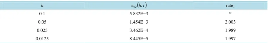
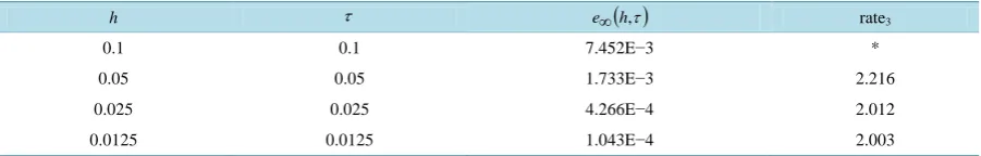
are sufficiently small.

By computing the problems (5.1)-(5.2) with the difference schemes (2.4)-(2.6), we carry out the spatial and temporal convergence in the sense of the maximum norm. Table 1 and Table 2 give the errors between numeri-cal solutions and exact solutions for spatial and temporal convergence, respectively. Once again, we conclude from Tables 1-3, that the difference schemes (2.4)-(2.6) are convergent with the convergence order of two both in space and in time. This is in accordance with Theorem 2.

6. Conclusion

[image:7.595.86.539.646.719.2]

In this paper, we use the discrete energy method to study the convergence of a linearized difference scheme for solving the two-dimensional Sivashinsky equation. The convergence is proved to be second order in the maxi-

Table 1.The spatial convergence orders in maximum norm for difference schemes (2.1)-(2.3) to the inhomogeneous Siva-shinsky Equations (5.1) and (5.2), with τ=0.0025.

h e∞( )h,τ rate1

0.1 5.832E−3 *

0.05 1.454E−3 2.003

0.025 3.462E−4 1.989

(8)

[image:8.595.89.537.112.187.2]

Table 2. The temporal convergence orders in maximum norm for difference schemes (2.1)-(2.3) to the inhomogeneous Si-vashinsky Equations (5.1) and (5.2), with h=0.0025.

h e∞( )h,τ rate2

0.1 8.745E−4 *

0.05 1.913E−4 2.187

0.025 4.115E−5 2.274

0.0125 9.570E−6 2.042

Table 3. The maximum norm errors and convergence orders for difference schemes (2.1)-(2.3) to the inhomogeneous Siva-shinsky Equations (5.1) and (5.2).

h τ e∞( )h,τ rate3

0.1 0.1 7.452E−3 *

0.05 0.05 1.733E−3 2.216

0.025 0.025 4.266E−4 2.012

0.0125 0.0125 1.043E−4 2.003

mum norm, which extends the result in [3][4] where they only prove the second order convergence of the dif-ference scheme for one-dimensional Sivashinsky equation in the discrete L2-norm. For obtaining the approx-imate solution for the two dimensional Sivashinsky equation by finite element Galerkin method, one must need polynomials of the degree ≥3. It means that they have to construct minimum 10 node triangle for approximat-ing the solution. Computationally, it is very expensive and difficult to impose inter-element C1 continuity con-dition. If the boundary is curved, imposition of boundary conditions causes some more difficulties. Therefore, based on the linearized difference schemes (2.4)-(2.6), this article proposes a recipe to eradicate such numerical difficulties.

References

[1] Sivashinsky, G.I. (1983) On Cellular Instability in the Solidification of a Dilute Binary Alloy. Physica 8D, North-Hol- land Publishing Company, Amsterdam, 243-248. http://dx.doi.org/10.1016/0167-2789(83)90321-4

[2] Gertsberg, V.G. and Sivashinsky, G.I. (1981) Large Cells in Nonlinear Rayleigh-Bénard Convection. Progress of Theoretical Physics, 66, 1219-1229. http://dx.doi.org/10.1143/PTP.66.1219

[3] Omrani, K. (2003) A Second-Order Splitting Method for a Finite Difference Scheme for the Sivashinsky Equation.

Applied Mathematics Letters, 16, 441-445. http://dx.doi.org/10.1016/S0893-9659(03)80070-8

[4] Omrani, K. and Mohamed, M.B. (2005) A Linearized Difference Scheme for the Sivashinsky Equation. Far East Jour- nal of Applied Mathematics, 20, 179-188.

[5] Omrani, K. (2007) Numerical Methods and Error Analysis for the Nonlinear Sivashinsky Equation. Applied Mathe-matics and Computation, 189, 949-962. http://dx.doi.org/10.1016/j.amc.2006.11.169

[6] Khiari, N., Achouri, T., Mohamed, M.L.B. and Omrani, K. (2007) Finite Difference Approximate Solutions for the Cahn-Hilliard Equation. Numerical Methods for Partial Differential Equations, 23, 437-455.

http://dx.doi.org/10.1002/num.20189

[7] Atouani, N. and Omrani, K. (2015) On the Convergence of Conservative Difference Schemes for the 2D Generalized Rosenau-Korteweg de Vries Equation. Applied Mathematics and Computation, 250, 832-847.

http://dx.doi.org/10.1016/j.amc.2014.10.106

[8] Atouani, N. and Omrani, K. (2015) A New Conservative High-Order Accurate Difference Scheme for the Rosenau Equation. Applicable Analysis, 94, 2435-2455. http://dx.doi.org/10.1080/00036811.2014.987134

[9] Omrani, K., Abidi, F., Achouri, T. and Khiari, N. (2008) A New Conservative Finite Difference Scheme for the Rose-nau Equation. Applied Mathematics and Computation, 201, 35-43. http://dx.doi.org/10.1016/j.amc.2007.11.039 [10] Khiari, N. and Omrani, K. (2011) Finite difference Discretization of the Extended Fisher-Kolmogorov Equation in

Two Dimension. Computers and Mathematics with Applications, 62, 4151-4160. http://dx.doi.org/10.1016/j.camwa.2011.09.065

[image:8.595.88.539.222.294.2]

(9)

for the Usual Rosenau-RLW Equation. Applied Mathematical Modelling, 36, 3371-3378. http://dx.doi.org/10.1016/j.apm.2011.08.022

[12] Pan, X. and Zhang, L. (2012) Numerical Simulation for General Rosenau-RLW Equation: An Average Linearized Conservative Scheme. Mathematical Problems in Engineering, 2012, Article ID: 517818.

http://dx.doi.org/10.1155/2012/517818

[13] Hu, J., Xu, Y. and Hu, B. (2013) Conservative Linear Difference Scheme for Rosenau-KdV Equation. Advances in Mathematical Physics, 2013, Article ID: 423718.http://dx.doi.org/10.1155/2013/423718

[14] Zhao, X, Liu, F and Liu, B (2014) Finite Difference Discretization of a Fourth-Order Parabolic Equation Describing Crystal Surface Growth. Applicable Analysis, 94, 1964-1975.http://dx.doi.org/10.1080/00036811.2014.959440 [15] Sun, Z.Z. (2005) Numerical Methods of the Partial Differential Equations. Sciences Press, Beijing.

[16] Sun, Z.Z. (1995) A Second-Order Accurate Linearized Difference Scheme for the Two-Dimensional Cahn-Hilliard Equation. Mathematics of Computation, 212, 1463-1471.